Last updated: 2022-10-26

Checks: 7 0

Knit directory: locust-phase-transition-RNAseq/

This reproducible R Markdown analysis was created with workflowr (version 1.7.0). The Checks tab describes the reproducibility checks that were applied when the results were created. The Past versions tab lists the development history.

R Markdown file: up-to-date

Great! Since the R Markdown file has been committed to the Git repository, you know the exact version of the code that produced these results.

Environment: empty

Great job! The global environment was empty. Objects defined in the global environment can affect the analysis in your R Markdown file in unknown ways. For reproduciblity it’s best to always run the code in an empty environment.

Seed: set.seed(20221025)

The command set.seed(20221025) was run prior to running the code in the R Markdown file. Setting a seed ensures that any results that rely on randomness, e.g. subsampling or permutations, are reproducible.

Session information: recorded

Great job! Recording the operating system, R version, and package versions is critical for reproducibility.

Cache: none

Nice! There were no cached chunks for this analysis, so you can be confident that you successfully produced the results during this run.

File paths: relative

Great job! Using relative paths to the files within your workflowr project makes it easier to run your code on other machines.

Repository version: efef2c6

Great! You are using Git for version control. Tracking code development and connecting the code version to the results is critical for reproducibility.

The results in this page were generated with repository version efef2c6. See the Past versions tab to see a history of the changes made to the R Markdown and HTML files.

Note that you need to be careful to ensure that all relevant files for the analysis have been committed to Git prior to generating the results (you can use wflow_publish or wflow_git_commit). workflowr only checks the R Markdown file, but you know if there are other scripts or data files that it depends on. Below is the status of the Git repository when the results were generated:


Ignored files:
    Ignored:    .DS_Store
    Ignored:    analysis/.DS_Store
    Ignored:    data/.DS_Store
    Ignored:    data/americana/.DS_Store
    Ignored:    data/americana/STAR_counts_4thcol/.DS_Store
    Ignored:    data/cancellata/.DS_Store
    Ignored:    data/cancellata/STAR_counts_4thcol/.DS_Store
    Ignored:    data/cubense/.DS_Store
    Ignored:    data/cubense/STAR_counts_4thcol/.DS_Store
    Ignored:    data/gregaria/.DS_Store
    Ignored:    data/gregaria/STAR_counts_4thcol/.DS_Store
    Ignored:    data/gregaria/list/.DS_Store
    Ignored:    data/metadata/.DS_Store
    Ignored:    data/nitens/.DS_Store
    Ignored:    data/nitens/STAR_counts_4thcol/.DS_Store
    Ignored:    data/piceifrons/.DS_Store
    Ignored:    data/piceifrons/STAR_counts_4thcol/.DS_Store
    Ignored:    data/piceifrons/list/.DS_Store

Note that any generated files, e.g. HTML, png, CSS, etc., are not included in this status report because it is ok for generated content to have uncommitted changes.

These are the previous versions of the repository in which changes were made to the R Markdown (analysis/readmap-gregaria.Rmd) and HTML (docs/readmap-gregaria.html) files. If you’ve configured a remote Git repository (see ?wflow_git_remote), click on the hyperlinks in the table below to view the files as they were in that past version.

File	Version	Author	Date	Message
html	28b9817	MaevaTecher	2022-10-26	Build site.
html	80b25f8	MaevaTecher	2022-10-26	Build site.
html	b381b7e	MaevaTecher	2022-10-26	Build site.
html	5ec6089	MaevaTecher	2022-10-26	Build site.
Rmd	0e211f0	MaevaTecher	2022-10-26	wflow_publish(c("analysis/readmap-gregaria.Rmd"), republish = TRUE)

This document was written in R Markdown, and translated into html using the R package knitr. Press the buttons labelled Code to show or hide the R code used to produce each table, plot or statistical result. You can also select Show all code at the top of the page.

Load R libraries (install first from CRAN or Bioconductor)

library("knitr")
library("rmdformats")
library("tidyverse")
library("DT")  # for making interactive search table
library("plotly") # for interactive plots
library("ggthemes") # for theme_calc
library("reshape2")

## Global options
options(max.print="10000")
knitr::opts_chunk$set(
    echo = TRUE,
    message = FALSE,
    warning = FALSE,
    cache = FALSE,
    comment = FALSE,
    prompt = FALSE,
    tidy = TRUE
)
opts_knit$set(width=75)

1 | Brief background: locust phase polyphenism

add description here

2 | Preparation for the analysis

2.1. Use a conda environment

add what to install on the Macpro tower e.g., we install a conda environment called rna-seq

2.2. Use modules on TAMU Grace cluster

We use a Snakemake pipeline for each species. Therefore, verifying that the software is installed as a module beforehand on the Grace cluster at Texas A&M University is essential. In addition, each module requires some dependencies, which is why we need to ensure they will be loaded together.

For this we use the function module spider [targeted software] w/o the version.

knitr::include_graphics("assets/module_spider.png", error = FALSE)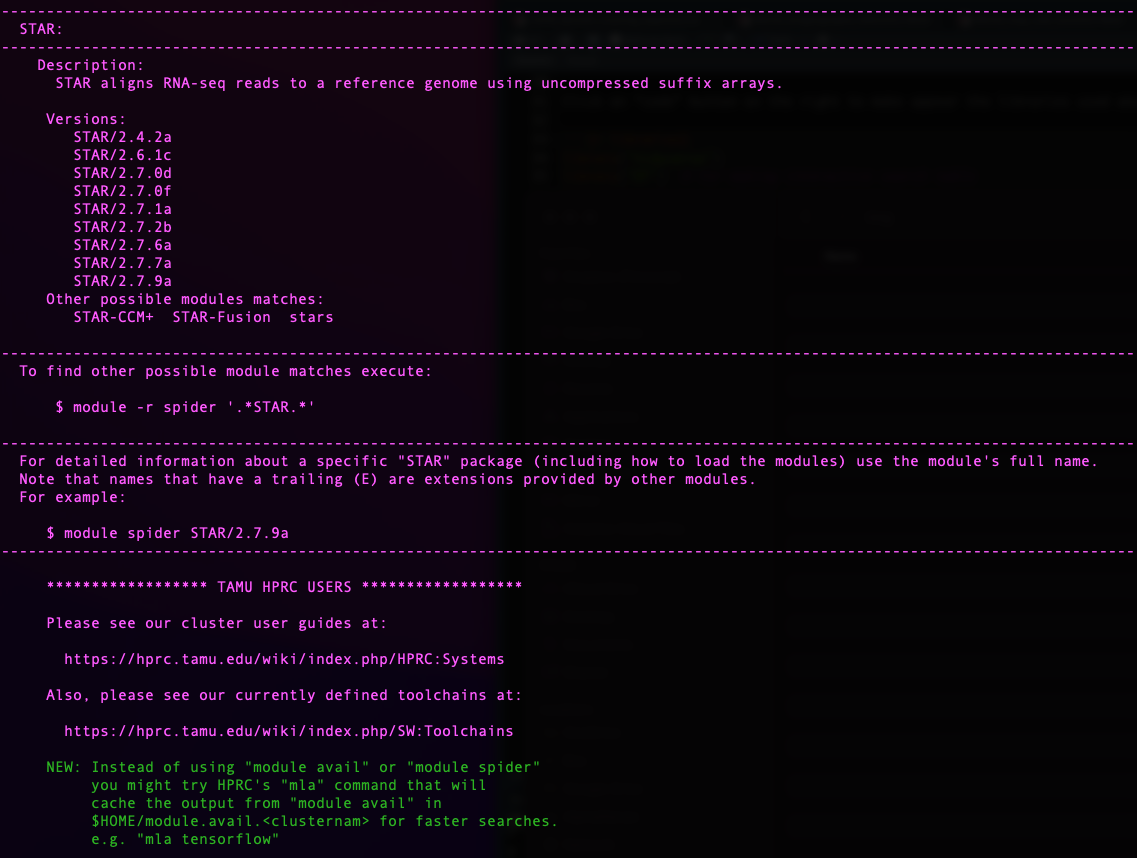

Version	Author	Date
770a79c	MaevaTecher	2022-10-26

Today we will need the following software:

to launch the Snakemake pipeline

module load GCC/11.2.0 OpenMPI/4.1.1 snakemake/6.10.0 Biopython/1.79

to perform adapter trimming and QC

module load Trimmomatic/0.39-Java-11
module load FastQC/0.11.9-Java-11

to perform short read mapping

module load GCC/11.2.0 STAR/2.7.9a

2.3. De novo sequencing

We generated new whole transcriptomes from two density conditions for the desert locust (Acrididae: Schistocerca gregaria). Here, we analyze 20 transcriptomes for a pilot project using Illumina Stranded Total RNA with RiboZero depletion and sequenced on a NovaSeq SP flow cell at TxGen.

The details of the sequences are as follow:
Bulk tissue from 2nd generation solitary control
GREG-HATCH-S1-FULL_S20: Solitary hatch-ling 1st instar from Pearl and Atticus
GREG-S-ICT-9-ALB_S6: Antenna lobes from replicate #9
GREG-S-ICT-9-ANT_S5: Antennae from replicate #9
GREG-S-ICT-9-FAT_S3: Fat body from replicate #9
GREG-S-ICT-9-MHB_S7: Mushroom body from replicate #9
GREG-S-ICT-9-MOP_S4: Maxillary palps from replicate #9
GREG-S-ICT-9-MTG_S2: Metathoracic ganglia from replicate #9
GREG-S-ICT-9-OLB_S8: Optical lobes from replicate #9
GREG-S-ICT-9-WG_S1: Whole gut from replicate #9

Bulk tissue from highly crowded control
GREG-G-CCT-11-ALB_S14: Antenna lobes from replicate #11
GREG-G-CCT-11-ALB-FULL_S17: Antenna lobes from replicate #11
GREG-G-CCT-11-ANT_S13: Antennae from replicate #11
GREG-G-CCT-11-FAT_S11: Fat body from replicate #11
GREG-G-CCT-11-FAT-FULL_S19: Fat body from replicate #11
GREG-G-CCT-11-MHB_S15: Mushroom body from replicate #11
GREG-G-CCT-11-MOP_S12: Maxillary palps from replicate #11
GREG-G-CCT-11-MTG_S10: Metathoracic ganglia from replicate #11
GREG-G-CCT-11-OLB_S16: Optical lobes from replicate #11
GREG-G-CCT-11-OLB-FULL_S18: Optical lobes from replicate #11
GREG-G-CCT-11-WG_S9: Whole gut from replicate #11

2.4. Downloading NCBI SRAs

We searched through the NCBI database for RNA SRA associated with Schistocerca in general and found 160 accessions were available.

Using the Run Selector from NCBI, we can easily download a metadata table which we can use to visualize how the accessions are distributed per species. We will use this metadata table for analysis in which we include pre-generated SRA.

We collect a list of accessions from Run for each species and then use SRA-toolkit from NCBI. First, we make an empty directory named ncbi to download each SRA. This is where SRA Toolkit will dump the prefetched SRA files in .sra format.

ml purge
ml GCC/10.2.0 OpenMPI/4.0.5 SRA-Toolkit/2.10.9
vdb-config --interactive

Once in the vdb-config interactive mode, select cache, choose, then use [ .. ], to enter /home/USERNAME/PATH/ncbi one directory at a time

prefetch --option-file SraAccList.txt
cat SraAccList.txt | xargs fasterq-dump --split-3 --outdir "/your-directory/for-fastq"

Clean-up the ncbi directory and move the fastq.gz file (rename if wanted).

another option

for x in *.sra ; do fasterq-dump --split-files $x ; mv *.fastq ../../paired_end_piceifrons/; done

3 | Locust transcriptomes mapping

3.1. Preparing the metadata file

Make a .csv file with as much information as possible per sample/file name (e.g., Sample_ID, Species, Sex, RearingCondition). An interactive and searchable table is found below and even be downloaded directly.

NB: Throughout our analysis, we will complete this metadata file by adding other stats related to sequencing and mapping.

# Load our SRA metadata table
metaseq <- read_table("data/metadata/RNAseq_modified_METADATA2022.txt", col_names = TRUE,
    guess_max = 5000)

## Create an interactive search table
metaseq %>%
    datatable(extensions = "Buttons", options = list(dom = "Blfrtip", buttons = c("copy",
        "csv", "excel"), lengthMenu = list(c(10, 20, 50, 100, 200, -1), c(10, 20,
        50, 100, 200, "All"))))

3.2. Repository and Snakefile

We will use from here our Snakemake pipeline that we will customize by launching small individual jobs to tailor each cluster parameter for the best memory and time efficiency.

To ease the indexing of our file and folder, we generate some shared parameters which will be helpful in the future: 1) reference genome directory path REFdir, 2) output directory path OUTdir and 3) a list LOCUSTS containing sample base name referred as locust.

### SET DIRECTORY PATHS FOR REFERENCE AND OUTPUT DATA

REFdir = "/scratch/user/maeva-techer/refgenomes"
OUTdir = "/scratch/user/maeva-techer/locust-rna/data"

### SAMPLES LIST AND OTHER PARAMETERS

LOCUSTS, = glob_wildcards(OUTdir + "/reads/{locust}_1.fastq.gz")
print(LOCUSTS)

3.3. Trim and adapter removal

From the point we have the renamed, and paired-end / single-end read for the species of interest (one folder), we will now run our Snakemake pipeline on it. If not done beforehand, we need to check randomly the quality of the sequences downloaded or generated using FASTQC. After our quick check, we can determine any parameters change for Trimmomatic.

########################################
# Snakefile rule
########################################

rule trim_adapt:
    input:
        read1 = OUTdir + "/reads/{locust}_1.fastq.gz",
        read2 = OUTdir + "/reads/{locust}_2.fastq.gz",
        adaptfile = OUTdir + "/list/TruSeqNextera_PE.fa"
    output:
        trimmedread1 = OUTdir + "/trimming/{locust}_trim1P_1.fastq.gz",
        badread1 = OUTdir + "/trimming/{locust}_trim1U_1.fastq.gz",
        trimmedread2 = OUTdir + "/trimming/{locust}_trim2P_2.fastq.gz",
        badread2 = OUTdir + "/trimming/{locust}_trim2U_2.fastq.gz",
    shell:
        """
        module load Trimmomatic/0.39-Java-11
        java -jar $EBROOTTRIMMOMATIC/trimmomatic-0.39.jar PE -threads 2 -phred33 {input.read1} {input.read2} {output.trimmedread1} {output.badread1} {output.trimmedread2} {output.badread2} ILLUMINACLIP:{input.adaptfile}:2:30:10 LEADING:30 TRAILING:30 SLIDINGWINDOW:4:15 MINLEN:36 
        """
        
########################################
# Parameters in the cluster.json file
########################################

    "trim_adapt":
    {
        "cpus-per-task" : 2,
        "partition" : "medium",
    "ntasks": 2,
        "mem" : "1G",
        "time": "0-04:00:00"
    },

3.4. Trim quality control

We always QC after trimming to ensure fine-tuning that the sequences clipping and filtering were not unnecessarily harsh. Given the number of sequences we work with, we do not need to go through each file immediately for time purposes. Instead, sample randomly across species, rearing conditions, and tissues to see that the process worked well.

########################################
# Snakefile rule
########################################

#Quality control step after trimming: checked for adapter content in particular and quality scores
rule trim_fastqc:
    input:
        read1 = OUTdir + "/trimming/{locust}_trim1P_1.fastq.gz",
        read2 = OUTdir + "/trimming/{locust}_trim2P_2.fastq.gz",
    output:
        htmlqc1 = OUTdir + "/trimming/{locust}_trim1P_1_fastqc.html",
        htmlqc2 = OUTdir + "/trimming/{locust}_trim2P_2_fastqc.html",
    shell:
        """
        module load FastQC/0.11.9-Java-11
        fastqc {input.read1}
        fastqc {input.read2}
        """
        
########################################
# Parameters in the cluster.json file
########################################

    "trim_fastqc":
    {
        "cpus-per-task" : 2,
        "partition" : "medium",
        "ntasks": 1,
        "mem" : "500M",
        "time": "0-03:00:00"
    },

3.5. Short Reads mapping

We used STAR for mapping reads to either 1) their own species reference genome or 2) an alternate sister reference genome. The pipeline is the same, except that the code will change index.

########################################
# Snakefile rule
########################################

#Ahead of the alignment I will build independently the index for STAR, HiSat2 and Segemehl

rule STAR_align:
    input:
        index = REFdir + "/locusts_complete/index_GCF_021461395.2_iqSchAmer2.1_genomic/STAR",
        read1 = OUTdir + "/trimming/{locust}_trim1P_1.fastq.gz",
        read2 = OUTdir + "/trimming/{locust}_trim2P_2.fastq.gz"
    params:
        prefix = OUTdir + "/alignment/STAR/{locust}_"
    output:
        OUTdir + "/alignment/STAR/{locust}_Aligned.sortedByCoord.out.bam"
    shell:
        """
        module load GCC/11.2.0 STAR/2.7.9a
        STAR --runThreadN 8 --genomeDir {input.index} --outSAMtype BAM SortedByCoordinate --quantMode GeneCounts --outFileNamePrefix {params.prefix} --readFilesCommand zcat --readFilesIn {input.read1} {input.read2} 
        """
        
########################################
# Parameters in the cluster.json file
########################################

    "STAR_align":
    {
        "cpus-per-task" : 12,
        "partition" : "medium",
        "ntasks": 1,
        "mem" : "100G",
        "time": "0-08:00:00"
    }

After mapping, we obtained alignment statistics from the *_Log.final.out file and filled out the metadata table with it.

grep 'Number of input reads' *_Log.final.out
grep 'Average input read length' *_Log.final.out
grep 'Uniquely mapped reads number' *_Log.final.out
grep 'Number of reads mapped to multiple loci' *_Log.final.out
grep 'Number of reads mapped to too many loci' *_Log.final.out
grep 'Number of reads unmapped: too many mismatches' *Log.final.out
grep 'Number of reads unmapped: too short' *Log.final.out
grep 'Number of reads unmapped: other' *Log.final.out

Map to own species

mycol_species <- c("green", "deeppink", "orange", "orange2", "blue2", "red2", "yellow2")

## READS AVERAGE colored by STATUS
eren <- ggplot(metaseq, aes(x = Map_SUM, y = Inputtrim_reads, color = Species, label = SampleID))
eren <- eren + geom_point(size = 2, alpha = 0.7)
eren <- eren + scale_color_manual(values = mycol_species)
eren <- eren + theme_calc()
eren <- eren + geom_hline(yintercept = 3e+07, linetype = "dotted", color = "green3")
eren <- eren + geom_hline(yintercept = 5e+07, linetype = "dotted", color = "green3")
eren <- eren + geom_vline(xintercept = 80, linetype = "dotted", color = "blue2")
eren <- eren + xlim(0, 100)
options(scipen = 20)  #to remove the scientific annotation of the axis

## make an interactive version of the scatter plot
attacktitan <- ggplotly(eren)
attacktitan

Figure XX: Interactive plot of the mapping rate success of each sample against their respective reference genome.

We added the green thresholds to indicate how many reads are recommended by Illumina (lower end and optimal). The blue line demonstrates where the mapping ratio could be considered not contaminated.

Map to gregaria

## READS AVERAGE colored by STATUS
mikasa <- ggplot(metaseq, aes(x = Map_SUM, y = Inputtrim_reads, color = Species,
    label = SampleID))
mikasa <- mikasa + geom_point(size = 2, alpha = 0.7)
mikasa <- mikasa + scale_color_manual(values = mycol_species)
mikasa <- mikasa + theme_calc()
mikasa <- mikasa + geom_hline(yintercept = 30000000, linetype = "dotted", color = "green3")
mikasa <- mikasa + geom_hline(yintercept = 50000000, linetype = "dotted", color = "green3")
mikasa <- mikasa + geom_vline(xintercept = 80, linetype = "dotted", color = "blue2")
mikasa <- mikasa + xlim(0, 100)
options(scipen = 20)  #to remove the scientific annotation of the axis

## make an interactive version of the scatter plot
attacktitan <- ggplotly(eren)
attacktitan

Figure XX: Interactive plot of the mapping rate success of each sample against gregaria genome.

We added the green thresholds to indicate how many reads are recommended by Illumina (lower end and optimal). The blue line demonstrates where the mapping ratio could be considered not contaminated.

Map to piceifrons

Map to cancellata

Map to americana

Map to cubense

Map to nitens

3.6. Quantification

We can note that the option --quantMode GeneCounts from STAR produces the same output as the htseq-count tool if we used the –-sjdbGTFfile option.

In the output file {locust}_ReadsPerGene.out.tab we can obtain the read counts per gene depending if our data is unstranded (column 2) or stranded (columns 3 and 4).

column 1: gene ID
column 2: counts for unstranded RNA-seq.
column 3: counts for the 1st read strand aligned with RNA
column 4: counts for the 2nd read strand aligned with RNA (the most common protocol nowadays)

For our pilot S. gregaria project, we know we used Illumina stranded kit but to check we can with the following code:

grep -v "N_" {locust}_ReadsPerGene.out.tab | awk '{unst+=$2;forw+=$3;rev+=$4}END{print unst,forw,rev}'

#or as a loop
for i in *_ReadsPerGene.out.tab; do echo $i; grep -v "N_" $i | awk '{unst+=$2;forw+=$3;rev+=$4}END{print unst,forw,rev}'; done

In a stranded library preparation protocol, there should be a strong imbalance between number of reads mapped to known genes in forward versus reverse strands. This is what we observe for example on S. cancellata libraries here.

PREFERRED OPTION: We need to extract in our case the 1st and 4th columns for each file.

########################################
# Snakefile rule
########################################

#either ran the following rule
rule reads_count:
        input:
                readtable = OUTdir + "/alignment/STAR2/{locust}_ReadsPerGene.out.tab",
        output:
                OUTdir + "/DESeq2/counts_4thcol/{locust}_counts.txt"
        shell:
                """
                cut -f1,4 {input.readtable} | grep -v "_" > {output}  
                """

#or simply this loop for less core usage
# for i in $SCRATCH/locust_phase/data/alignment/STAR/*ReadsPerGene.out.tab; do echo $i; cut -f1,4 $i | grep -v "_" > $SCRATCH/locust_phase/data/DESeq2/counts_4thcol/`basename $i ReadsPerGene.out.tab`counts.txt; done

ALTERNATIVE OPTION: We can also build a single matrix of expression with all individuals targeted. Below is the example for S. piceifrons:

paste SPICE_*_ReadsPerGene.out.tab | grep -v "_" | awk '{printf "%s\t", $1}{for (i=4;i<=NF;i+=4) printf "%s\t", $i; printf "\n" }' > tmp
sed -e "1igene_name\t$(ls SPICE_*ReadsPerGene.out.tab | tr '\n' '\t' | sed 's/_ReadsPerGene.out.tab//g')" tmp > raw_counts_piceifrons_matrix.txt

sessionInfo()

FALSE R version 4.2.1 (2022-06-23)
FALSE Platform: x86_64-apple-darwin17.0 (64-bit)
FALSE Running under: macOS Big Sur ... 10.16
FALSE 
FALSE Matrix products: default
FALSE BLAS:   /Library/Frameworks/R.framework/Versions/4.2/Resources/lib/libRblas.0.dylib
FALSE LAPACK: /Library/Frameworks/R.framework/Versions/4.2/Resources/lib/libRlapack.dylib
FALSE 
FALSE locale:
FALSE [1] en_US.UTF-8/en_US.UTF-8/en_US.UTF-8/C/en_US.UTF-8/en_US.UTF-8
FALSE 
FALSE attached base packages:
FALSE [1] stats     graphics  grDevices utils     datasets  methods   base     
FALSE 
FALSE other attached packages:
FALSE  [1] reshape2_1.4.4   ggthemes_4.2.4   plotly_4.10.0    DT_0.26         
FALSE  [5] forcats_0.5.2    stringr_1.4.1    dplyr_1.0.10     purrr_0.3.5     
FALSE  [9] readr_2.1.3      tidyr_1.2.1      tibble_3.1.8     ggplot2_3.3.6   
FALSE [13] tidyverse_1.3.2  rmdformats_1.0.4 knitr_1.40       workflowr_1.7.0 
FALSE 
FALSE loaded via a namespace (and not attached):
FALSE  [1] fs_1.5.2            lubridate_1.8.0     httr_1.4.4         
FALSE  [4] rprojroot_2.0.3     tools_4.2.1         backports_1.4.1    
FALSE  [7] bslib_0.4.0         utf8_1.2.2          R6_2.5.1           
FALSE [10] DBI_1.1.3           lazyeval_0.2.2      colorspace_2.0-3   
FALSE [13] withr_2.5.0         tidyselect_1.2.0    processx_3.7.0     
FALSE [16] compiler_4.2.1      git2r_0.30.1        cli_3.4.1          
FALSE [19] rvest_1.0.3         formatR_1.12        xml2_1.3.3         
FALSE [22] labeling_0.4.2      bookdown_0.29       sass_0.4.2         
FALSE [25] scales_1.2.1        callr_3.7.2         digest_0.6.30      
FALSE [28] rmarkdown_2.17      pkgconfig_2.0.3     htmltools_0.5.3    
FALSE [31] dbplyr_2.2.1        fastmap_1.1.0       highr_0.9          
FALSE [34] htmlwidgets_1.5.4   rlang_1.0.6         readxl_1.4.1       
FALSE [37] rstudioapi_0.14     jquerylib_0.1.4     generics_0.1.3     
FALSE [40] jsonlite_1.8.3      crosstalk_1.2.0     googlesheets4_1.0.1
FALSE [43] magrittr_2.0.3      Rcpp_1.0.9          munsell_0.5.0      
FALSE [46] fansi_1.0.3         lifecycle_1.0.3     stringi_1.7.8      
FALSE [49] whisker_0.4         yaml_2.3.6          plyr_1.8.7         
FALSE [52] grid_4.2.1          promises_1.2.0.1    crayon_1.5.2       
FALSE [55] haven_2.5.1         hms_1.1.2           ps_1.7.1           
FALSE [58] pillar_1.8.1        reprex_2.0.2        glue_1.6.2         
FALSE [61] evaluate_0.17       getPass_0.2-2       data.table_1.14.4  
FALSE [64] modelr_0.1.9        vctrs_0.5.0         tzdb_0.3.0         
FALSE [67] httpuv_1.6.6        cellranger_1.1.0    gtable_0.3.1       
FALSE [70] assertthat_0.2.1    cachem_1.0.6        xfun_0.34          
FALSE [73] broom_1.0.1         later_1.3.0         googledrive_2.0.0  
FALSE [76] viridisLite_0.4.1   gargle_1.2.1        ellipsis_0.3.2

transcriptome-mapping-analysis2

Maeva Techer

2022-10-26