Differential Gene Expression Workflow
Maeva Techer
2022-10-31
Last updated: 2022-10-31
Checks: 7 0
Knit directory:
locust-phase-transition-RNAseq/
This reproducible R Markdown analysis was created with workflowr (version 1.7.0). The Checks tab describes the reproducibility checks that were applied when the results were created. The Past versions tab lists the development history.
Great! Since the R Markdown file has been committed to the Git repository, you know the exact version of the code that produced these results.
Great job! The global environment was empty. Objects defined in the global environment can affect the analysis in your R Markdown file in unknown ways. For reproduciblity it’s best to always run the code in an empty environment.
The command set.seed(20221025) was run prior to running
the code in the R Markdown file. Setting a seed ensures that any results
that rely on randomness, e.g. subsampling or permutations, are
reproducible.
Great job! Recording the operating system, R version, and package versions is critical for reproducibility.
Nice! There were no cached chunks for this analysis, so you can be confident that you successfully produced the results during this run.
Great job! Using relative paths to the files within your workflowr project makes it easier to run your code on other machines.
Great! You are using Git for version control. Tracking code development and connecting the code version to the results is critical for reproducibility.
The results in this page were generated with repository version 2ccb4bc. See the Past versions tab to see a history of the changes made to the R Markdown and HTML files.
Note that you need to be careful to ensure that all relevant files for
the analysis have been committed to Git prior to generating the results
(you can use wflow_publish or
wflow_git_commit). workflowr only checks the R Markdown
file, but you know if there are other scripts or data files that it
depends on. Below is the status of the Git repository when the results
were generated:
Ignored files:
    Ignored:    .DS_Store
    Ignored:    analysis/.DS_Store
    Ignored:    data/.DS_Store
    Ignored:    data/americana/.DS_Store
    Ignored:    data/americana/STAR_counts_4thcol/.DS_Store
    Ignored:    data/cancellata/.DS_Store
    Ignored:    data/cancellata/STAR_counts_4thcol/.DS_Store
    Ignored:    data/cubense/.DS_Store
    Ignored:    data/cubense/STAR_counts_4thcol/.DS_Store
    Ignored:    data/gregaria/.DS_Store
    Ignored:    data/gregaria/STAR_counts_4thcol/.DS_Store
    Ignored:    data/gregaria/list/.DS_Store
    Ignored:    data/metadata/.DS_Store
    Ignored:    data/nitens/.DS_Store
    Ignored:    data/nitens/STAR_counts_4thcol/.DS_Store
    Ignored:    data/piceifrons/.DS_Store
    Ignored:    data/piceifrons/STAR_counts_4thcol/.DS_Store
    Ignored:    data/piceifrons/list/.DS_Store

Unstaged changes:
    Deleted:    analysis/gene-quant.Rmd
    Deleted:    analysis/own-refseq.Rmd
Note that any generated files, e.g. HTML, png, CSS, etc., are not included in this status report because it is ok for generated content to have uncommitted changes.
These are the previous versions of the repository in which changes were
made to the R Markdown (analysis/deg-workflow.Rmd) and HTML
(docs/deg-workflow.html) files. If you’ve configured a
remote Git repository (see ?wflow_git_remote), click on the
hyperlinks in the table below to view the files as they were in that
past version.
| File | Version | Author | Date | Message |
|---|---|---|---|---|
| Rmd | 2ccb4bc | MaevaTecher | 2022-10-31 | wflow_publish(c("analysis/_site.yml", "data/gregaria/list/BrainPilot.txt", |
Load required R libraries
#(install first from CRAN or Bioconductor)
library("knitr")
library("rmdformats")
library("tidyverse")
library("DT")  # for making interactive search table
library("plotly") # for interactive plots
library("ggthemes") # for theme_calc
library("reshape2")
library("DESeq2")
library("data.table")
library("apeglm")
library("ggpubr")
library("ggplot2")
library("ggrepel")
library("EnhancedVolcano")

## Global options
options(max.print="10000")
knitr::opts_chunk$set(
    echo = TRUE,
    message = FALSE,
    warning = FALSE,
    cache = FALSE,
    comment = FALSE,
    prompt = FALSE,
    tidy = TRUE
)
opts_knit$set(width=75)
Here we present the workflow example with the head data from S. piceifrons
For the analysis of differentially expressed genes, we will follow
some guidelines from an online RNA course tutorial
that uses either DESeq2 or edgeR on STAR
output.
DESeq2 tests for differential expression using negative binomial generalized linear models. DESeq2 (as edgeR) is based on the hypothesis that most genes are not differentially expressed. The package takes as an input raw counts (i.e. non normalized counts): the DESeq2 model internally corrects for library size, so giving as an input normalized count would be incorrect.
DGE analysis with STAR input
Preparing input files
Raw count matrices
We generated this in the precedent section.
Transcript-to-gene annotation file
Below is the example with S. gregaria
# Download annotation and place it into the folder refgenomes
wget https://ftp.ncbi.nlm.nih.gov/genomes/all/GCF/023/897/955/GCF_023897955.1_iqSchGreg1.2/GCF_023897955.1_iqSchGreg1.2_genomic.gtf.gz

# first column is the transcript ID, second column is the gene ID, third column is the gene symbol
zcat GCF_023897955.1_iqSchGreg1.2_genomic.gtf.gz | awk -F "\t" 'BEGIN{OFS="\t"}{if($3=="transcript"){split($9, a, "\""); print a[4],a[2],a[8]}}' > tx2gene.gregaria.csv
Sample sheet
DESeq2 needs a sample sheet that describes the samples characteristics: SampleName, FileName (…counts.txt), and subsequently anything that can be used for statistical design such as RearingCondition, replicates, tissue, time points, etc. in the form.
The design indicates how to model the samples: in the model we need to specify what we want to measure and what we want to control.
Differential expression analysis
Import input count data
We start by reading the sample sheet.
## import the sample sheet that indicates Rearing Conditions and Tissue origins
sampletable <- fread("data/piceifrons/list/HeadSPICE.txt")
# add the sample names as row names (it is needed for some of the DESeq
# functions)
rownames(sampletable) <- sampletable$SampleName

# Make sure discriminant variables are factor
sampletable$RearingCondition <- as.factor(sampletable$RearingCondition)
sampletable$Tissue <- as.factor(sampletable$Tissue)
dim(sampletable)
FALSE [1] 10 4Then we obtain the output from STAR GeneCount and import
here individually using the sampletable as a reference to fetch them. We
also filter the lowly expressed genes to avoid noisy data.
# Read in the two-column data.frame linking transcript id (column 1) to gene id
# (column 2)
tx2gene <- read.table("data/piceifrons/list/tx2gene.piceifrons.csv", sep = "\t",
    header = F)

satoshi <- DESeqDataSetFromHTSeqCount(sampleTable = sampletable, directory = "data/piceifrons/STAR_counts_4thcol",
    design = ~RearingCondition)

satoshi
FALSE class: DESeqDataSet
FALSE dim: 28731 10
FALSE metadata(1): version
FALSE assays(1): counts
FALSE rownames(28731): LOC124794980 LOC124795035 ... LOC124774866
FALSE LOC124774858
FALSE rowData names(0):
FALSE colnames(10): SPICE_G_Crd_SRR11815268 SPICE_G_Crd_SRR11815269 ...
FALSE SPICE_S_Iso_SRR11815273 SPICE_S_Iso_SRR11815274
FALSE colData names(2): Tissue RearingCondition# keep genes for which sums of raw counts across experimental samples is > 5
satoshi <- satoshi[rowSums(counts(satoshi)) > 5, ]
nrow(satoshi)FALSE [1] 14932# set a standard to be compared to (hatchling) ONLY IF WE HAVE A CONTROL
# satoshi$Tissue <- relevel(satoshi$Tissue, ref = 'Whole_body')Run the model Fit DESeq2
Run DESeq2 analysis using DESeq, which performs (1)
estimation of size factors, (2) estimation of dispersion, then (3)
Negative Binomial GLM fitting and Wald statistics. The results tables
(log2 fold changes and p-values) can be generated using the results
function (copied
from online chapter)
# Fit the statistical model
shigeru <- DESeq(satoshi)
cbind(resultsNames(shigeru))
FALSE [,1]
FALSE [1,] "Intercept"
FALSE [2,] "RearingCondition_Isolated_vs_Crowded"# Here we plot the adjusted p-value means corrected for multiple testing (FDR
# padj)
res_shigeru <- results(shigeru)
# We only keep genes with an adjusted p-value cutoff > 0.05 by changing the
# default significance cut-off sum(res_shigeru$padj < 0.05, na.rm = TRUE)
brock <- results(shigeru, name = "RearingCondition_Isolated_vs_Crowded", alpha = 0.05)
summary(brock)FALSE
FALSE out of 14932 with nonzero total read count
FALSE adjusted p-value < 0.05
FALSE LFC > 0 (up) : 254, 1.7%
FALSE LFC < 0 (down) : 404, 2.7%
FALSE outliers [1] : 497, 3.3%
FALSE low counts [2] : 1156, 7.7%
FALSE (mean count < 2)
FALSE [1] see 'cooksCutoff' argument of ?results
FALSE [2] see 'independentFiltering' argument of ?results# Details of what is each column meaning in our final result
mcols(brock)$descriptionFALSE [1] "mean of normalized counts for all samples"
FALSE [2] "log2 fold change (MLE): RearingCondition Isolated vs Crowded"
FALSE [3] "standard error: RearingCondition Isolated vs Crowded"
FALSE [4] "Wald statistic: RearingCondition Isolated vs Crowded"
FALSE [5] "Wald test p-value: RearingCondition Isolated vs Crowded"
FALSE [6] "BH adjusted p-values"head(brock)FALSE log2 fold change (MLE): RearingCondition Isolated vs Crowded
FALSE Wald test p-value: RearingCondition Isolated vs Crowded
FALSE DataFrame with 6 rows and 6 columns
FALSE baseMean log2FoldChange lfcSE stat pvalue
FALSE <numeric> <numeric> <numeric> <numeric> <numeric>
FALSE LOC124796288 2.37306 -3.529621 1.337214 -2.639533 8.30204e-03
FALSE LOC124796294 1.14866 -2.301130 2.134062 -1.078286 2.80906e-01
FALSE LOC124796332 9.18581 -0.600937 0.715740 -0.839603 4.01131e-01
FALSE LOC124793320 133.76396 -1.759458 0.613514 -2.867835 4.13290e-03
FALSE LOC124712404 29.00252 -1.601387 1.002767 -1.596968 NA
FALSE LOC124798649 11.86003 5.205485 0.872809 5.964059 2.46048e-09
FALSE padj
FALSE <numeric>
FALSE LOC124796288 1.10023e-01
FALSE LOC124796294 NA
FALSE LOC124796332 7.40311e-01
FALSE LOC124793320 7.03370e-02
FALSE LOC124712404 NA
FALSE LOC124798649 6.40640e-07For this data set after FDR filtering of 0.05, we have 254 genes up-regulates and 404 genes down-regulated in crowded versus solitary individuals.
Visualizing and exploring the results
PCA of the samples
We transformed the data for visualization by comparing both recommended rlog (Regularized log) or vst (Variance Stabilizing Transformation) transformations. Both options produce log2 scale data which has been normalized by the DESeq2 method with respect to library size.
# Try with the vst transformation
shigeru_vsd <- vst(shigeru)
shigeru_rlog <- rlog(shigeru)
Plot the PCA rlog
# Create the pca on the defined groups
pcaData <- plotPCA(object = shigeru_rlog, intgroup = c("RearingCondition", "Tissue"),
    returnData = TRUE)

# Store the information for each axis variance in %
percentVar <- round(100 * attr(pcaData, "percentVar"))

# Make sure that the discriminant variable are in factor for using shape and
# color later on
pcaData$RearingCondition <- factor(pcaData$RearingCondition, levels = c("Crowded",
    "Isolated"), labels = c("crowded piceifrons", "isolated piceifrons"))
levels(pcaData$RearingCondition)
FALSE [1] "crowded piceifrons" "isolated piceifrons"# pcaData$Tissue<-factor(pcaData1$Tissue,levels=c('Whole_body','Optical_lobes'),
# labels=c('Hatchling', 'OLB')) levels(pcaData$Tissue)
ggplot(pcaData, aes(PC1, PC2, color = RearingCondition)) + geom_point(size = 4) +
xlab(paste0("PC1: ", percentVar[1], "% variance")) + ylab(paste0("PC2: ", percentVar[2],
"% variance")) + scale_color_manual(values = c("blue", "red")) + geom_text_repel(aes(label = name),
nudge_x = -1, nudge_y = 0.2, size = 3) + coord_fixed() + theme_bw() + theme(legend.title = element_blank()) +
theme(legend.text = element_text(face = "bold", size = 15)) + theme(axis.text = element_text(size = 15)) +
theme(axis.title = element_text(size = 16)) + ggtitle("PCA on S. piceifrons head tissues",
subtitle = "rlog transformation") + xlab(paste0("PC1: ", percentVar[1], "% variance")) +
ylab(paste0("PC2: ", percentVar[2], "% variance"))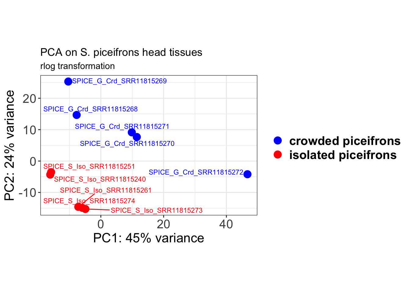
Plot the PCA vsd
# Create the pca on the defined groups
pcaData <- plotPCA(object = shigeru_vsd, intgroup = c("RearingCondition", "Tissue"),
    returnData = TRUE)

# Store the information for each axis variance in %
percentVar <- round(100 * attr(pcaData, "percentVar"))

# Make sure that the discriminant variable are in factor for using shape and
# color later on
pcaData$RearingCondition <- factor(pcaData$RearingCondition, levels = c("Crowded",
    "Isolated"), labels = c("crowded piceifrons", "isolated piceifrons"))
levels(pcaData$RearingCondition)
FALSE [1] "crowded piceifrons" "isolated piceifrons"# pcaData$Tissue<-factor(pcaData1$Tissue,levels=c('Whole_body','Optical_lobes'),
# labels=c('Hatchling', 'OLB')) levels(pcaData$Tissue)
ggplot(pcaData, aes(PC1, PC2, color = RearingCondition)) + geom_point(size = 4) +
xlab(paste0("PC1: ", percentVar[1], "% variance")) + ylab(paste0("PC2: ", percentVar[2],
"% variance")) + scale_color_manual(values = c("blue", "red")) + geom_text_repel(aes(label = name),
nudge_x = -1, nudge_y = 0.2, size = 3) + coord_fixed() + theme_bw() + theme(legend.title = element_blank()) +
theme(legend.text = element_text(face = "bold", size = 15)) + theme(axis.text = element_text(size = 15)) +
theme(axis.title = element_text(size = 16)) + ggtitle("PCA on S. piceifrons head tissues",
subtitle = "vst transformation") + xlab(paste0("PC1: ", percentVar[1], "% variance")) +
ylab(paste0("PC2: ", percentVar[2], "% variance"))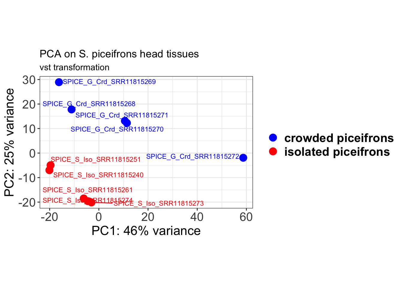
MA-plot
This plot allows us to show the log2 fold changes over the mean of normalized counts for all the samples. Points will be colored in red if the adjusted p-value is less than 0.05 and the log2 fold change is bigger than 1. In blue, will be the reverse for the log2 fold change.
# include the log2FoldChange shrinkage use to visualize gene ranking
de_shrink <- lfcShrink(dds = shigeru, coef = "RearingCondition_Isolated_vs_Crowded",
    type = "apeglm")

# Ma plot
maplot <- ggmaplot(de_shrink, fdr = 0.05, fc = 1, size = 1.5, palette = c("#B31B21",
    "#1465AC", "darkgray"), genenames = as.vector(rownames(de_shrink$name)), top = 0,
    legend = "top", label.select = NULL) + coord_cartesian(xlim = c(0, 18)) + scale_y_continuous(limits = c(-8,
    8)) + theme(axis.text.x = element_text(size = 16), axis.text.y = element_text(size = 15),
    axis.title.x = element_text(size = 17), axis.title.y = element_text(size = 17),
    axis.line = element_line(size = 1, colour = "gray20"), axis.ticks = element_line(size = 1,
        colour = "gray20")) + guides(color = guide_legend(override.aes = list(size = c(3,
    3, 3)))) + theme(legend.position = c(0.7, 0.12), legend.text = element_text(size = 14,
    face = "bold"), legend.background = element_rect(fill = "transparent")) + theme(plot.title = element_text(size = 18,
    colour = "gray30", face = "bold", hjust = 0.06, vjust = -5)) + labs(title = "MA-plot for the shrunken log2 fold changes in the head")
maplot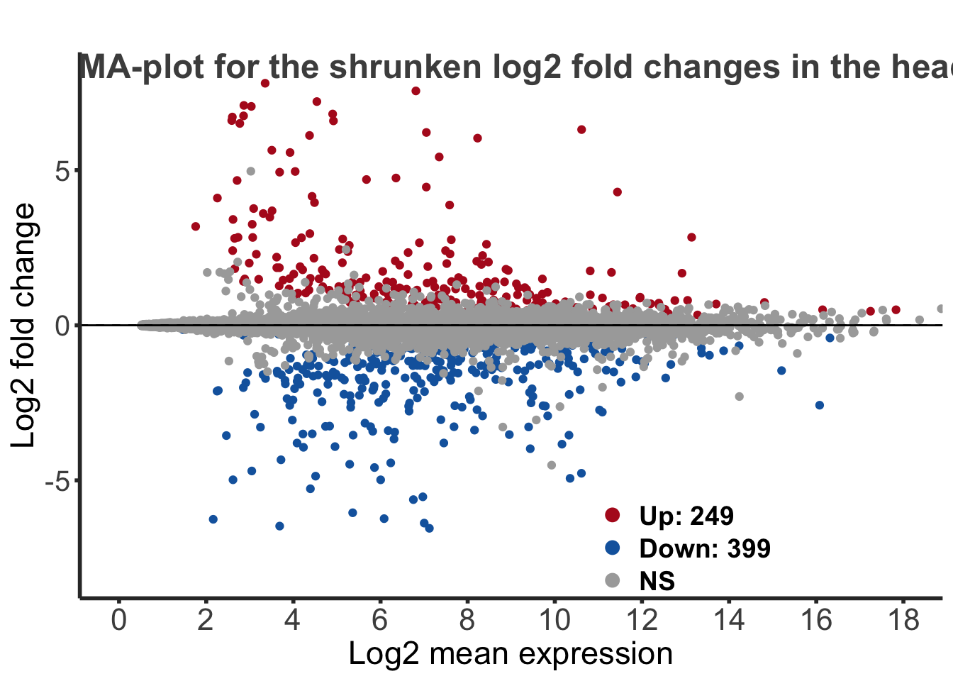
The EnhancedVolcano helps visualise the resulst of
differential expression analysis.
keyvals <- ifelse(res_shigeru$log2FoldChange >= 1 & res_shigeru$padj <= 0.05, "red",
    ifelse(res_shigeru$log2FoldChange <= -1 & res_shigeru$padj <= 0.05, "green",
        "black"))

keyvals[is.na(keyvals)] <- "black"
names(keyvals)[keyvals == "red"] <- "Upregulated"
names(keyvals)[keyvals == "green"] <- "Downregulated"
names(keyvals)[keyvals == "black"] <- "NS"

EnhancedVolcano(res_shigeru, lab = rownames(res_shigeru), x = "log2FoldChange", y = "padj",
    pCutoff = 0.05, FCcutoff = 1, pointSize = 3, labSize = 3, colAlpha = 4/5, colCustom = keyvals,
    drawConnectors = FALSE)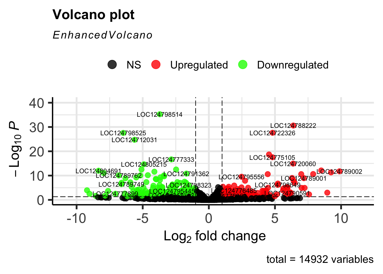
sessionInfo()FALSE R version 4.2.1 (2022-06-23)
FALSE Platform: x86_64-apple-darwin17.0 (64-bit)
FALSE Running under: macOS Big Sur ... 10.16
FALSE
FALSE Matrix products: default
FALSE BLAS: /Library/Frameworks/R.framework/Versions/4.2/Resources/lib/libRblas.0.dylib
FALSE LAPACK: /Library/Frameworks/R.framework/Versions/4.2/Resources/lib/libRlapack.dylib
FALSE
FALSE locale:
FALSE [1] en_US.UTF-8/en_US.UTF-8/en_US.UTF-8/C/en_US.UTF-8/en_US.UTF-8
FALSE
FALSE attached base packages:
FALSE [1] stats4 stats graphics grDevices utils datasets methods
FALSE [8] base
FALSE
FALSE other attached packages:
FALSE [1] EnhancedVolcano_1.14.0 ggrepel_0.9.1
FALSE [3] ggpubr_0.4.0 apeglm_1.18.0
FALSE [5] data.table_1.14.4 DESeq2_1.36.0
FALSE [7] SummarizedExperiment_1.26.1 Biobase_2.56.0
FALSE [9] MatrixGenerics_1.8.1 matrixStats_0.62.0
FALSE [11] GenomicRanges_1.48.0 GenomeInfoDb_1.32.4
FALSE [13] IRanges_2.31.2 S4Vectors_0.34.0
FALSE [15] BiocGenerics_0.42.0 reshape2_1.4.4
FALSE [17] ggthemes_4.2.4 plotly_4.10.0
FALSE [19] DT_0.26 forcats_0.5.2
FALSE [21] stringr_1.4.1 dplyr_1.0.10
FALSE [23] purrr_0.3.5 readr_2.1.3
FALSE [25] tidyr_1.2.1 tibble_3.1.8
FALSE [27] ggplot2_3.3.6 tidyverse_1.3.2
FALSE [29] rmdformats_1.0.4 knitr_1.40
FALSE [31] workflowr_1.7.0
FALSE
FALSE loaded via a namespace (and not attached):
FALSE [1] readxl_1.4.1 backports_1.4.1 plyr_1.8.7
FALSE [4] lazyeval_0.2.2 splines_4.2.1 BiocParallel_1.30.4
FALSE [7] digest_0.6.30 htmltools_0.5.3 fansi_1.0.3
FALSE [10] magrittr_2.0.3 memoise_2.0.1 googlesheets4_1.0.1
FALSE [13] tzdb_0.3.0 Biostrings_2.64.1 annotate_1.74.0
FALSE [16] modelr_0.1.9 bdsmatrix_1.3-6 colorspace_2.0-3
FALSE [19] blob_1.2.3 rvest_1.0.3 haven_2.5.1
FALSE [22] xfun_0.34 callr_3.7.2 crayon_1.5.2
FALSE [25] RCurl_1.98-1.9 jsonlite_1.8.3 genefilter_1.78.0
FALSE [28] survival_3.4-0 glue_1.6.2 gtable_0.3.1
FALSE [31] gargle_1.2.1 zlibbioc_1.42.0 XVector_0.36.0
FALSE [34] DelayedArray_0.22.0 car_3.1-1 abind_1.4-5
FALSE [37] scales_1.2.1 mvtnorm_1.1-3 DBI_1.1.3
FALSE [40] rstatix_0.7.0 Rcpp_1.0.9 viridisLite_0.4.1
FALSE [43] xtable_1.8-4 emdbook_1.3.12 bit_4.0.4
FALSE [46] htmlwidgets_1.5.4 httr_1.4.4 RColorBrewer_1.1-3
FALSE [49] ellipsis_0.3.2 farver_2.1.1 pkgconfig_2.0.3
FALSE [52] XML_3.99-0.11 sass_0.4.2 dbplyr_2.2.1
FALSE [55] locfit_1.5-9.6 utf8_1.2.2 labeling_0.4.2
FALSE [58] tidyselect_1.2.0 rlang_1.0.6 later_1.3.0
FALSE [61] AnnotationDbi_1.58.0 munsell_0.5.0 cellranger_1.1.0
FALSE [64] tools_4.2.1 cachem_1.0.6 cli_3.4.1
FALSE [67] generics_0.1.3 RSQLite_2.2.18 broom_1.0.1
FALSE [70] evaluate_0.17 fastmap_1.1.0 yaml_2.3.6
FALSE [73] processx_3.7.0 bit64_4.0.5 fs_1.5.2
FALSE [76] KEGGREST_1.36.3 whisker_0.4 formatR_1.12
FALSE [79] xml2_1.3.3 compiler_4.2.1 rstudioapi_0.14
FALSE [82] png_0.1-7 ggsignif_0.6.4 reprex_2.0.2
FALSE [85] geneplotter_1.74.0 bslib_0.4.0 stringi_1.7.8
FALSE [88] highr_0.9 ps_1.7.1 lattice_0.20-45
FALSE [91] Matrix_1.5-1 vctrs_0.5.0 pillar_1.8.1
FALSE [94] lifecycle_1.0.3 jquerylib_0.1.4 bitops_1.0-7
FALSE [97] httpuv_1.6.6 R6_2.5.1 bookdown_0.29
FALSE [100] promises_1.2.0.1 codetools_0.2-18 MASS_7.3-58.1
FALSE [103] assertthat_0.2.1 rprojroot_2.0.3 withr_2.5.0
FALSE [106] GenomeInfoDbData_1.2.8 parallel_4.2.1 hms_1.1.2
FALSE [109] grid_4.2.1 coda_0.19-4 rmarkdown_2.17
FALSE [112] carData_3.0-5 googledrive_2.0.0 git2r_0.30.1
FALSE [115] getPass_0.2-2 bbmle_1.0.25 numDeriv_2016.8-1.1
FALSE [118] lubridate_1.8.0