Transcriptome sequencing data pre-processing
Maeva Techer
2024-02-19
Last updated: 2024-02-19
Checks: 7 0
Knit directory:
locust-comparative-genomics/
This reproducible R Markdown analysis was created with workflowr (version 1.7.1). The Checks tab describes the reproducibility checks that were applied when the results were created. The Past versions tab lists the development history.
Great! Since the R Markdown file has been committed to the Git repository, you know the exact version of the code that produced these results.
Great job! The global environment was empty. Objects defined in the global environment can affect the analysis in your R Markdown file in unknown ways. For reproduciblity it’s best to always run the code in an empty environment.
The command set.seed(20221025) was run prior to running
the code in the R Markdown file. Setting a seed ensures that any results
that rely on randomness, e.g. subsampling or permutations, are
reproducible.
Great job! Recording the operating system, R version, and package versions is critical for reproducibility.
Nice! There were no cached chunks for this analysis, so you can be confident that you successfully produced the results during this run.
Great job! Using relative paths to the files within your workflowr project makes it easier to run your code on other machines.
Great! You are using Git for version control. Tracking code development and connecting the code version to the results is critical for reproducibility.
The results in this page were generated with repository version 55f9385. See the Past versions tab to see a history of the changes made to the R Markdown and HTML files.
Note that you need to be careful to ensure that all relevant files for
the analysis have been committed to Git prior to generating the results
(you can use wflow_publish or
wflow_git_commit). workflowr only checks the R Markdown
file, but you know if there are other scripts or data files that it
depends on. Below is the status of the Git repository when the results
were generated:
Ignored files:
    Ignored:    .DS_Store
    Ignored:    .RData
    Ignored:    .Rhistory
    Ignored:    .Rproj.user/
    Ignored:    analysis/.DS_Store
    Ignored:    analysis/.Rhistory
    Ignored:    data/.DS_Store
    Ignored:    data/.Rhistory
    Ignored:    data/metadata/.DS_Store
    Ignored:    figures/
Note that any generated files, e.g. HTML, png, CSS, etc., are not included in this status report because it is ok for generated content to have uncommitted changes.
These are the previous versions of the repository in which changes were
made to the R Markdown (analysis/3_seq-data-qc.Rmd) and
HTML (docs/3_seq-data-qc.html) files. If you’ve configured
a remote Git repository (see ?wflow_git_remote), click on
the hyperlinks in the table below to view the files as they were in that
past version.
| File | Version | Author | Date | Message |
|---|---|---|---|---|
| Rmd | 55f9385 | Maeva A. TECHER | 2024-02-19 | wflow_publish("analysis/3_seq-data-qc.Rmd") |
| html | df94db2 | Maeva A. TECHER | 2024-02-19 | adding markdown qc |
| Rmd | f6b4961 | Maeva A. TECHER | 2024-02-19 | wflow_publish("analysis/3_seq-data-qc.Rmd") |
| html | e39d280 | Maeva A. TECHER | 2024-01-29 | Build site. |
| html | f701a01 | Maeva A. TECHER | 2024-01-29 | reupdate |
| html | be046c6 | Maeva A. TECHER | 2024-01-24 | Build site. |
| html | 1b09cbe | Maeva A. TECHER | 2024-01-24 | remove |
| html | 141b63c | Maeva A. TECHER | 2023-12-18 | Build site. |
| Rmd | 53877fa | Maeva A. TECHER | 2023-12-18 | add pages |
At this point, we will have organized both SRA and de novo
paired-end sequencing data within our reads directory located
at
/scratch/group/songlab/maeva/headthor-locusts-rna/{species}/data/reads
and will be ready to run the Snakemake pipeline on it. As a reminder,
each library corresponds to the transcriptome of bulk tissues (either
head or thorax) from a single specimen reared under isolated or crowded
conditions.
Load R libraries (install first from CRAN or Bioconductor)
library("knitr")
library("rmdformats")
library("tidyverse")
library("DT")  # for making interactive search table
library("plotly") # for interactive plots
library("ggthemes") # for theme_calc
library("reshape2")
library("readr")
library("ggplot2")

## Global options
options(max.print="10000")
knitr::opts_chunk$set(
    echo = TRUE,
    message = FALSE,
    warning = FALSE,
    cache = FALSE,
    comment = FALSE,
    prompt = FALSE,
    tidy = TRUE
)
opts_knit$set(width=75)
Control the quality of the .fastq files
The first step is to ensure that we have enough reads per library and
remove any potential outlier resulting from library preparation or
sequencing failure. For that, we will assess each .fastq file with
FASTQC. However, considering we are working with a
significant sample size, we will compile the results using
MULTIQC.
The aggregated results can be conveniently viewed by opening the HTML report in a web browser.
module load GCC/12.2.0  OpenMPI/4.1.4 MultiQC/1.14
multiqc --title 'TYPE THE TITLE YOU WANT' -v /PATHTODIRECTORY
montana <- read_table("data/metadata/Stats_RNAseq_QC_19Feb2024.txt", col_names = TRUE, guess_max = 1000)
head(montana)FALSE # A tibble: 6 × 7
FALSE Sample_Name Species Perc_Dups Perc_GC M_Seqs Unique_Reads Duplicate_Reads
FALSE <chr> <chr> <dbl> <dbl> <dbl> <dbl> <dbl>
FALSE 1 SAMER_G_Crd_SRR… americ… 0.71 0.46 23.7 6958831 16765516
FALSE 2 SAMER_G_Crd_SRR… americ… 0.67 0.47 23.7 7784916 15939431
FALSE 3 SAMER_G_Crd_SRR… americ… 0.71 0.48 15.7 4570667 11085054
FALSE 4 SAMER_G_Crd_SRR… americ… 0.67 0.48 15.7 5145265 10510456
FALSE 5 SAMER_G_Crd_SRR… americ… 0.84 0.49 37.2 6049864 31125514
FALSE 6 SAMER_G_Crd_SRR… americ… 0.8 0.49 37.2 7301268 29874110# Convert values to millions
montana <- montana %>%
mutate_at(vars(contains("Reads")), list(~ ./1000000))
# Pivot the data
montana_long <- montana %>%
pivot_longer(cols = contains("Reads"), names_to = "Variable", values_to = "Value")
# Define colors
colors.reads <- c("Duplicate_Reads" = "black", "Unique_Reads" = "deepskyblue")
# Plot the stacked bar plot with values in millions and custom colors
ggplot(montana_long, aes(x = Sample_Name, y = Value, fill = Variable)) +
geom_bar(stat = "identity", position = "stack") +
facet_wrap(~Species, scales = "free") +
labs(title = "Stacked Bar Plot of Unique Reads and Duplicate Reads by Sample",
x = NULL, # Remove x-axis label
y = "Millions of Reads") +
theme_minimal() +
theme(axis.text.x = element_blank()) + # Remove x-axis labels
scale_fill_manual(values = colors.reads) + # Set custom colors
geom_hline(yintercept = 30, linetype = "dashed", color = "red") +
geom_hline(yintercept = 50, linetype = "dashed", color = "gray70") +
ylim(0, 62) # Set y-axis limits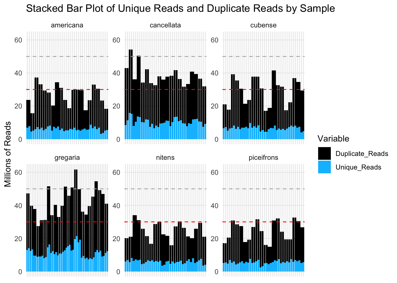
library(ggConvexHull)
# Define custom colors for each species
species_colors <- c("americana" = "forestgreen", "cubense" = "yellow3", "gregaria" = "orange", "nitens" = "blue", "piceifrons" = "red2", cancellata = "deeppink")

p <- ggplot(montana, aes(x = Perc_Dups, y = M_Seqs, color = Species)) +
  geom_point(size =2) +
  scale_color_manual(values = species_colors) +  # Apply custom colors
  labs(title = "M_Seqs vs % Dups by Species",
       x = "Percentage of Duplicates",
       y = "Millions of Reads") +
  theme_minimal()

p + geom_convexhull(aes(fill = Species, color = Species), alpha = 0.2) +
    scale_fill_manual(values = species_colors)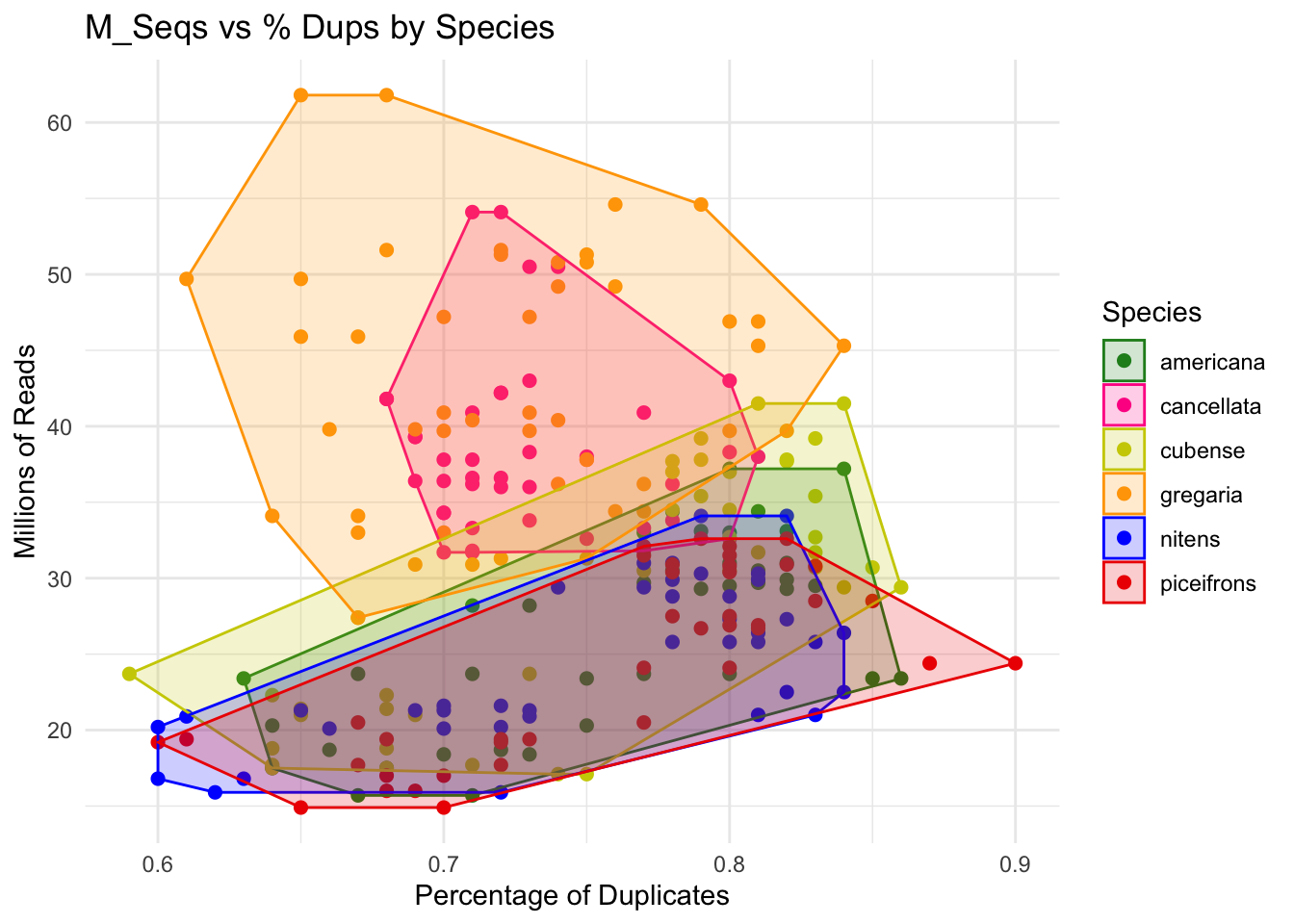
Trim and adapter removal
After checking the initial sequence quality, we can determine whether
any parameters adjustments are needed for Trimmomatic. This
is particularly pertinent for the ‘trailings’ and ‘leading’ parameters
which removes the nucleotides at the end and start
########################################
# Snakefile rule
########################################

rule trim_adapt:
    input:
        read1 = OUTdir + "/reads/{locust}_1.fastq.gz",
        read2 = OUTdir + "/reads/{locust}_2.fastq.gz",
        adaptfile = OUTdir + "/list/TruSeqNextera_PE.fa"
    output:
        trimmedread1 = OUTdir + "/trimming/{locust}_trim1P_1.fastq.gz",
        badread1 = OUTdir + "/trimming/{locust}_trim1U_1.fastq.gz",
        trimmedread2 = OUTdir + "/trimming/{locust}_trim2P_2.fastq.gz",
        badread2 = OUTdir + "/trimming/{locust}_trim2U_2.fastq.gz",
    shell:
        """
        module load Trimmomatic/0.39-Java-11
        java -jar $EBROOTTRIMMOMATIC/trimmomatic-0.39.jar PE -threads 2 -phred33 {input.read1} {input.read2} {output.trimmedread1} {output.badread1} {output.trimmedread2} {output.badread2} ILLUMINACLIP:{input.adaptfile}:2:30:10 LEADING:30 TRAILING:30 SLIDINGWINDOW:4:15 MINLEN:36
        """

########################################
# Parameters in the cluster.json file
########################################

    "trim_adapt":
    {
        "cpus-per-task" : 2,
        "partition" : "medium",
    "ntasks": 2,
        "mem" : "1G",
        "time": "0-04:00:00"
    },
SLIDINGWINDOWWe use the 4:15 approach which means that in a 4-base window, if the average quality drops below 15, the bases will be trimmed.MINLEN:36Specifies the minimum length a read must be to be kept after all trimming steps is at 36 bp otherwise it is too short to convey any information.
We used the Illumina adapters for library preparation and as per recommended on the support website, we removed TruSeq.
We created a list called TruSeqNextera_PE.fa that
gathered several adapters. >PrefixPE/1
TACACTCTTTCCCTACACGACGCTCTTCCGATCT >PrefixPE/2
GTGACTGGAGTTCAGACGTGTGCTCTTCCGATCT >PE1
TACACTCTTTCCCTACACGACGCTCTTCCGATCT >PE1_rc
AGATCGGAAGAGCGTCGTGTAGGGAAAGAGTGTA >PE2
GTGACTGGAGTTCAGACGTGTGCTCTTCCGATCT >PE2_rc
AGATCGGAAGAGCACACGTCTGAACTCCAGTCAC>PrefixNX/1 AGATGTGTATAAGAGACAG
>PrefixNX/2 AGATGTGTATAAGAGACAG >Trans1
TCGTCGGCAGCGTCAGATGTGTATAAGAGACAG >Trans1_rc
CTGTCTCTTATACACATCTGACGCTGCCGACGA >Trans2
GTCTCGTGGGCTCGGAGATGTGTATAAGAGACAG >Trans2_rc
CTGTCTCTTATACACATCTCCGAGCCCACGAGAC
Trim quality control
We always perform quality control checks after trimming to ensure that the clipping and filtering of sequences were not overly aggressive. Given the number of sequences we work with, manually inspecting each file immediately would be time-consuming. Instead, we adopt a random sampling approach across different species, rearing conditions, and tissues to see that the trimming process worked well.
########################################
# Snakefile rule
########################################

#Quality control step after trimming: checked for adapter content in particular and quality scores
rule trim_fastqc:
    input:
        read1 = OUTdir + "/trimming/{locust}_trim1P_1.fastq.gz",
        read2 = OUTdir + "/trimming/{locust}_trim2P_2.fastq.gz",
    output:
        htmlqc1 = OUTdir + "/trimming/{locust}_trim1P_1_fastqc.html",
        htmlqc2 = OUTdir + "/trimming/{locust}_trim2P_2_fastqc.html",
    shell:
        """
        module load FastQC/0.11.9-Java-11
        fastqc {input.read1}
        fastqc {input.read2}
        """

########################################
# Parameters in the cluster.json file
########################################

    "trim_fastqc":
    {
        "cpus-per-task" : 2,
        "partition" : "medium",
        "ntasks": 1,
        "mem" : "500M",
        "time": "0-03:00:00"
    },
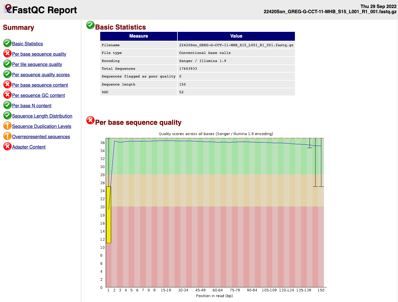
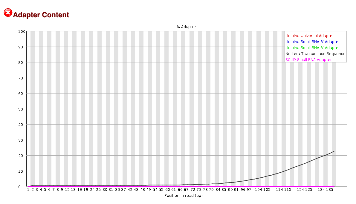
EXAMPLE OF READS QUALITY BEFORE TRIMMING
EXAMPLE OF READS QUALITY AFTER TRIMMING
We can see that the sequence length has changed and that the 5’ and 3’
end positions with lower quality have been removed.
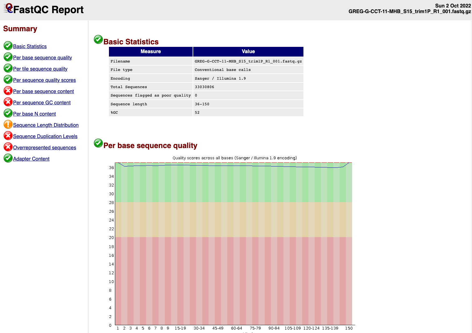
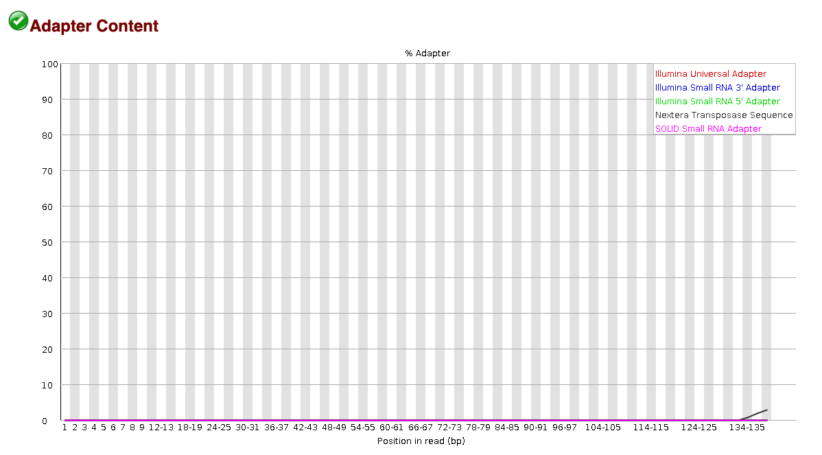
EXAMPLE OF READS QUALITY AFTER TRIMMING
We can see that most detected adapter sequences have been adequately removed after trimming.
Non-target sequencing data
Contamination is likely to occur throughout various stages of experiments, including tissue acquisition, RNA extraction and library preparation. One can hope to reduces as much as possible its impact on the final sequencing data which can affect the success rate of reads mapping.
Screen for microbial contamination
We decided to screen for microbes sequences present in the trimmed
paired-end reads FASTQ.gz files using the tool Kaiju.
Kaiju translates metatranscriptomics sequencing reads into
six possible reading frames and searches for maximum exact matches of
amino acid sequences in a given annotation protein database.
We used the most extensive microbial database nr_euk
which encompass the subset of NCBI BLAST nr database containing all
proteins belonging to Archaea, Bacteria, Viruses, Fungi and microbial
Eukaryotes.
## Downloading the 2022-03-10 database from Kaiju webserver
wget https://kaiju.binf.ku.dk/database/kaiju_db_nr_euk_2022-03-10.tgz
To run Kaiju we used the following
Snakemake rule:
########################################
# Snakefile rule
########################################

rule kaiju:
        input:
                read1 = OUTdir + "/trimming/{locust}_trim1P_1.fastq.gz",
                read2 = OUTdir + "/trimming/{locust}_trim2P_2.fastq.gz",
                database = KAIJUdir + "/kaiju_db_nr_euk.fmi",
                taxonid = KAIJUdir + "/nodes.dmp",
                taxonnames = KAIJUdir + "/names.dmp",
        output:
                report = OUTdir + "/kaiju/{locust}_kaiju.out",
                classification = OUTdir + "/kaiju/{locust}_kaiju.tsv",
    shell:
                """
                ml GCC/8.3.0  OpenMPI/3.1.4 Kaiju/1.7.3-Python-3.7.4
                kaiju -z 12 -v -a greedy -f {input.database} -t {input.taxonid} -i {input.read1} -j {input.read2} -o {output.report}
        kaiju2table -v -t {input.taxonid} -n {input.taxonnames} -r phylum -o {output.classification} {output.report}
        """


########################################
# Parameters in the cluster.json file
########################################

    "kaiju":
    {
        "cpus-per-task" : 6,
        "partition" : "medium",
        "ntasks": 2,
        "mem" : "200G",
        "time": "0-12:00:00"
   },
The ouput produced here allows us to see the percentage of reads that map to unclassified (likely our locust host here) and the percentage of microbial contamination ranked in a phylum level.
Visualize the metatranscriptomics result
Kaiju output can be exported to be view in a interactive
and hierarchical multi-layered pie-charts using Krona. The
results are generated by a .html page. We followed the Kaiju tutorial
on the Github page:
########################################
# Snakefile rule
########################################

rule krona:
        input:
                kaijuout = OUTdir + "/kaiju/{locust}_kaiju.out",
                taxonid = KAIJUdir + "/nodes.dmp",
        taxonnames = KAIJUdir + "/names.dmp",
        output:
                conversion = OUTdir + "/kaiju/{locust}_krona.out",
        webreport = OUTdir + "/kaiju/{locust}_krona.html",
        shell:
                """
                ml GCCcore/8.2.0 KronaTools/2.7.1
                kaiju2krona -t {input.taxonid} -n {input.taxonnames} -i {input.kaijuout} -o {output.conversion}
        ktImportText -o {output.webreport} {output.conversion}
                """


########################################
# Parameters in the cluster.json file
########################################

    "krona":
    {
        "cpus-per-task" : 2,
        "partition" : "short",
        "ntasks": 1,
        "mem" : "500M",
        "time": "0-0:10:00"
   },
Ribosomal RNA
sessionInfo()FALSE R version 4.3.1 (2023-06-16)
FALSE Platform: x86_64-apple-darwin20 (64-bit)
FALSE Running under: macOS Sonoma 14.1.2
FALSE
FALSE Matrix products: default
FALSE BLAS: /Library/Frameworks/R.framework/Versions/4.3-x86_64/Resources/lib/libRblas.0.dylib
FALSE LAPACK: /Library/Frameworks/R.framework/Versions/4.3-x86_64/Resources/lib/libRlapack.dylib; LAPACK version 3.11.0
FALSE
FALSE locale:
FALSE [1] en_US.UTF-8/en_US.UTF-8/en_US.UTF-8/C/en_US.UTF-8/en_US.UTF-8
FALSE
FALSE time zone: America/Chicago
FALSE tzcode source: internal
FALSE
FALSE attached base packages:
FALSE [1] stats graphics grDevices utils datasets methods base
FALSE
FALSE other attached packages:
FALSE [1] ggConvexHull_0.1.0 reshape2_1.4.4 ggthemes_5.0.0 plotly_4.10.4
FALSE [5] DT_0.31 lubridate_1.9.3 forcats_1.0.0 stringr_1.5.1
FALSE [9] dplyr_1.1.4 purrr_1.0.2 readr_2.1.5 tidyr_1.3.1
FALSE [13] tibble_3.2.1 ggplot2_3.4.4 tidyverse_2.0.0 rmdformats_1.0.4
FALSE [17] knitr_1.45 workflowr_1.7.1
FALSE
FALSE loaded via a namespace (and not attached):
FALSE [1] gtable_0.3.4 xfun_0.41 bslib_0.6.1 htmlwidgets_1.6.4
FALSE [5] processx_3.8.3 callr_3.7.3 tzdb_0.4.0 vctrs_0.6.5
FALSE [9] tools_4.3.1 ps_1.7.6 generics_0.1.3 fansi_1.0.6
FALSE [13] highr_0.10 pkgconfig_2.0.3 data.table_1.15.0 lifecycle_1.0.4
FALSE [17] farver_2.1.1 compiler_4.3.1 git2r_0.33.0 munsell_0.5.0
FALSE [21] getPass_0.2-4 httpuv_1.6.14 htmltools_0.5.7 sass_0.4.8
FALSE [25] yaml_2.3.8 lazyeval_0.2.2 crayon_1.5.2 later_1.3.2
FALSE [29] pillar_1.9.0 jquerylib_0.1.4 whisker_0.4.1 cachem_1.0.8
FALSE [33] tidyselect_1.2.0 digest_0.6.34 stringi_1.8.3 bookdown_0.37
FALSE [37] labeling_0.4.3 rprojroot_2.0.4 fastmap_1.1.1 grid_4.3.1
FALSE [41] colorspace_2.1-0 cli_3.6.2 magrittr_2.0.3 utf8_1.2.4
FALSE [45] withr_3.0.0 scales_1.3.0 promises_1.2.1 timechange_0.3.0
FALSE [49] rmarkdown_2.25 httr_1.4.7 hms_1.1.3 evaluate_0.23
FALSE [53] viridisLite_0.4.2 rlang_1.1.3 Rcpp_1.0.12 glue_1.7.0
FALSE [57] formatR_1.14 rstudioapi_0.15.0 jsonlite_1.8.8 R6_2.5.1
FALSE [61] plyr_1.8.9 fs_1.6.3