Enrichment Analysis: Mutant Vs Wild-Type
Steve Pederson
19 February, 2020
Last updated: 2020-02-19
Checks: 7 0
Knit directory: 20170327_Psen2S4Ter_RNASeq/
This reproducible R Markdown analysis was created with workflowr (version 1.6.0). The Checks tab describes the reproducibility checks that were applied when the results were created. The Past versions tab lists the development history.
Great! Since the R Markdown file has been committed to the Git repository, you know the exact version of the code that produced these results.
Great job! The global environment was empty. Objects defined in the global environment can affect the analysis in your R Markdown file in unknown ways. For reproduciblity it’s best to always run the code in an empty environment.
The command set.seed(20200119) was run prior to running the code in the R Markdown file. Setting a seed ensures that any results that rely on randomness, e.g. subsampling or permutations, are reproducible.
Great job! Recording the operating system, R version, and package versions is critical for reproducibility.
Nice! There were no cached chunks for this analysis, so you can be confident that you successfully produced the results during this run.
Great job! Using relative paths to the files within your workflowr project makes it easier to run your code on other machines.
Great! You are using Git for version control. Tracking code development and connecting the code version to the results is critical for reproducibility. The version displayed above was the version of the Git repository at the time these results were generated.
Note that you need to be careful to ensure that all relevant files for the analysis have been committed to Git prior to generating the results (you can use wflow_publish or wflow_git_commit). workflowr only checks the R Markdown file, but you know if there are other scripts or data files that it depends on. Below is the status of the Git repository when the results were generated:
Ignored files:
    Ignored:    .Rhistory
    Ignored:    .Rproj.user/
Note that any generated files, e.g. HTML, png, CSS, etc., are not included in this status report because it is ok for generated content to have uncommitted changes.
These are the previous versions of the R Markdown and HTML files. If you’ve configured a remote Git repository (see ?wflow_git_remote), click on the hyperlinks in the table below to view them.
| File | Version | Author | Date | Message |
|---|---|---|---|---|
| Rmd | 4d2af23 | Steve Ped | 2020-02-19 | Modified heatmap sizes & initial network layout |
| Rmd | 8fe35b0 | Steve Ped | 2020-02-19 | Added multiple heatmaps & UpSet plots |
| html | 679b10d | Steve Ped | 2020-02-19 | Rendered OXPHOS Plot |
| Rmd | 66ba4e0 | Steve Ped | 2020-02-19 | Added OXPHOS plot |
| html | e0288c6 | Steve Ped | 2020-02-19 | Generated enrichment tables |
| Rmd | 541fbf0 | Steve Ped | 2020-02-19 | Revised Hom Vs Het Enrichment |
| Rmd | 77f167d | Steve Ped | 2020-02-19 | Revised enrichment |
| html | 876e40f | Steve Ped | 2020-02-17 | Compiled after minor corrections |
| Rmd | 53ed0e3 | Steve Ped | 2020-02-17 | Corrected Ensembl Release |
| Rmd | f55be85 | Steve Ped | 2020-02-17 | Added commas |
| Rmd | 8f29458 | Steve Ped | 2020-02-17 | Minor tweaks to formatting |
| html | 9104ecd | Steve Ped | 2020-01-28 | First draft of Hom Vs Het |
| Rmd | 207cdc8 | Steve Ped | 2020-01-28 | Added code for Hom Vs Het Enrichment |
| Rmd | 468e6e3 | Steve Ped | 2020-01-28 | Ran enrichment of Mut Vs WT |
| html | 468e6e3 | Steve Ped | 2020-01-28 | Ran enrichment of Mut Vs WT |
| Rmd | 3a9933c | Steve Ped | 2020-01-28 | Finished Enrichment analysis on MutVsWt |
| html | 3a9933c | Steve Ped | 2020-01-28 | Finished Enrichment analysis on MutVsWt |
Setup
library(tidyverse)
library(magrittr)
library(edgeR)
library(scales)
library(pander)
library(goseq)
library(msigdbr)
library(AnnotationDbi)
library(RColorBrewer)
library(ngsReports)
library(fgsea)
library(metap)
library(UpSetR)
library(pheatmap)
theme_set(theme_bw())
panderOptions("table.split.table", Inf)
panderOptions("table.style", "rmarkdown")
panderOptions("big.mark", ",")samples <- read_csv("data/samples.csv") %>%
distinct(sampleName, .keep_all = TRUE) %>%
dplyr::select(sample = sampleName, sampleID, genotype) %>%
mutate(
genotype = factor(genotype, levels = c("WT", "Het", "Hom")),
mutant = genotype %in% c("Het", "Hom"),
homozygous = genotype == "Hom"
)
genoCols <- samples$genotype %>%
levels() %>%
length() %>%
brewer.pal("Set1") %>%
setNames(levels(samples$genotype))dgeList <- read_rds("data/dgeList.rds")
fit <- read_rds("data/fit.rds")
entrezGenes <- dgeList$genes %>%
dplyr::filter(!is.na(entrezid)) %>%
unnest(entrezid) %>%
dplyr::rename(entrez_gene = entrezid)formatP <- function(p, m = 0.0001){
out <- rep("", length(p))
out[p < m] <- sprintf("%.2e", p[p<m])
out[p >= m] <- sprintf("%.4f", p[p>=m])
out
}Introduction
Enrichment analysis for this dataset present some challenges. Despite normalisation to account for gene length and GC bias, some appeared to still be present in the final results. In addition, the confounding of incomplete rRNA removal with genotype may lead to other distortions in both DE genes and ranking statistics.
Two steps for enrichment analysis will be undertaken.
- Testing for enrichment within discrete sets of DE genes as defined in the previous steps
- Testing for enrichment within ranked lists, regardless of DE status or statistical significance, before integration of all enrichment analyses using Fisher’s method for combining p-values.
Testing for enrichment within discrete gene sets will be performed using goseq as this allows for the incorporation of a single covariate as a predictor of differential expression. GC content, gene length and correlation with rRNA removal can all be supplied as separate covariates.
Testing for enrichment with ranked lists will be performed using:
fryas this can take into account inter-gene correlations. Values supplied will be fitted values for each gene/sample as these have been corrected for GC and length biases.camera, which also accommodates inter-gene correlations. Values supplied will be fitted values for each gene/sample as these have been corrected for GC and length biases.fgseawhich is an R implementation of GSEA. This approach simply takes a ranked list and doesn’t directly account for correlations. However, the ranked list will be derived from analysis using CQN-normalisation so will be robust to these technical artefacts.
In the case of camera, inter-gene correlations will be calculated for each gene-set prior to analysis to ensure more conservative p-values are obtained.
Databases used for testing
Data was sourced using the msigdbr package. The initial database used for testing was the Hallmark Gene Sets, with mappings from gene-set to EntrezGene IDs performed by the package authors.
Hallmark Gene Sets
hm <- msigdbr("Danio rerio", category = "H")  %>%
  left_join(entrezGenes) %>%
  dplyr::filter(!is.na(gene_id)) %>%
  distinct(gs_name, gene_id, .keep_all = TRUE)
hmByGene <- hm %>%
  split(f = .$gene_id) %>%
  lapply(extract2, "gs_name")
hmByID <- hm %>%
  split(f = .$gs_name) %>%
  lapply(extract2, "gene_id")
Mappings are required from gene to pathway, and Ensembl identifiers were used to map from gene to pathway, based on the mappings in the previously used annotations (Ensembl Release 98). A total of 3,459 Ensembl IDs were mapped to pathways from the hallmark gene sets.
KEGG Gene Sets
kg <- msigdbr("Danio rerio", category = "C2", subcategory = "CP:KEGG")  %>%
  left_join(entrezGenes) %>%
  dplyr::filter(!is.na(gene_id)) %>%
  distinct(gs_name, gene_id, .keep_all = TRUE)
kgByGene <- kg  %>%
  split(f = .$gene_id) %>%
  lapply(extract2, "gs_name")
kgByID <- kg  %>%
  split(f = .$gs_name) %>%
  lapply(extract2, "gene_id")
The same mapping process was applied to KEGG gene sets. A total of 3,614 Ensembl IDs were mapped to pathways from the KEGG gene sets.
Gene Ontology Gene Sets
goSummaries <- url("https://uofabioinformaticshub.github.io/summaries2GO/data/goSummaries.RDS") %>%
  readRDS() %>%
  mutate(
    Term = Term(id),
    gs_name = Term %>% str_to_upper() %>% str_replace_all("[ -]", "_"),
    gs_name = paste0("GO_", gs_name)
    )
minPath <- 3
go <- msigdbr("Danio rerio", category = "C5") %>%
left_join(entrezGenes) %>%
dplyr::filter(!is.na(gene_id)) %>%
left_join(goSummaries) %>%
dplyr::filter(shortest_path >= minPath) %>%
distinct(gs_name, gene_id, .keep_all = TRUE)
goByGene <- go %>%
split(f = .$gene_id) %>%
lapply(extract2, "gs_name")
goByID <- go %>%
split(f = .$gs_name) %>%
lapply(extract2, "gene_id")For analysis of gene-sets from the GO database, gene-sets were restricted to those with 3 or more steps back to the ontology root terms. A total of 11,245 Ensembl IDs were mapped to pathways from restricted database of 8,834 GO gene sets.
gsSizes <- bind_rows(hm, kg, go) %>%
  dplyr::select(gs_name, gene_symbol, gene_id) %>%
  chop(c(gene_symbol, gene_id)) %>%
  mutate(gs_size = vapply(gene_symbol, length, integer(1)))
Enrichment in the DE Gene Set
deTable <- file.path("output", "psen2VsWT.csv") %>%
  read_csv() %>%
  mutate(
    entrezid = dgeList$genes$entrezid[gene_id]
  )
The first step of analysis using goseq, regardless of the gene-set, is estimation of the probability weight function (PWF) which quantifies the probability of a gene being considered as DE based on a single covariate. As GC content and length should have been accounted for during conditional-quantile normalisation, these were not required for any bias. However, the gene-level correlations with rRNA contamination were instead used a predictor of bias in selection of a gene as being DE.
rawFqc <- list.files(
  path = "data/0_rawData/FastQC/",
  pattern = "zip",
  full.names = TRUE
) %>%
  FastqcDataList()
gc <- getModule(rawFqc, "Per_sequence_GC") %>%
  group_by(Filename) %>%
  mutate(Freq = Count / sum(Count)) %>%
  ungroup()
gcDev <- gc %>%
  left_join(getGC(gcTheoretical, "Drerio", "Trans")) %>%
  mutate(
    sample = str_remove(Filename, "_R[12].fastq.gz"),
    resid = Freq - Drerio
  ) %>%
  left_join(samples) %>%
  group_by(sample) %>%
  summarise(
    ss = sum(resid^2),
    n = n(),
    sd = sqrt(ss / (n - 1))
  )
riboVec <- structure(gcDev$sd, names = gcDev$sample)
riboCors <- cpm(dgeList, log = TRUE) %>%
apply(1, function(x){
cor(x, riboVec[names(x)])
})Values were calculated as per the previous steps, using the logCPM values for each gene, with the sample-level standard deviations from the theoretical GC distribution being used as a measure of rRNA contamination. For estimation of the probability weight function, squared correlations were used to place negative and positive correlations on the same scale. This accounts for genes which are both negatively & positively biased by the presence of excessive rRNA. Clearly, the confounding of genotype with rRNA means that some genes driven by the genuine biology may be down-weighted under this approach.
riboPwf <- deTable %>%
  mutate(riboCors = riboCors[gene_id]^2) %>%
  dplyr::select(gene_id, DE, riboCors) %>%
  distinct(gene_id, .keep_all = TRUE) %>%
  with(
    nullp(
      DEgenes = structure(
        as.integer(DE), names = gene_id
      ),
      genome = "danRer10",
      id = "ensGene",
      bias.data = riboCors,
      plot.fit = FALSE
    )
  )
plotPWF(riboPwf, main = "Bias from rRNA proportions")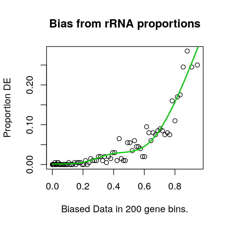
Using this approach, it was clear that correlation with rRNA proportions significantly biased the probability of a gene being considered as DE.
| Version | Author | Date |
|---|---|---|
| 468e6e3 | Steve Ped | 2020-01-28 |
All gene-sets were then tested using this PWF.
Hallmark Gene Sets
hmRiboGoseq <- goseq(riboPwf, gene2cat = hmByGene) %>%
  as_tibble %>%
  dplyr::filter(numDEInCat > 0) %>%
  mutate(
    adjP = p.adjust(over_represented_pvalue, method = "bonf"),
    FDR = p.adjust(over_represented_pvalue, method = "fdr")
  ) %>%
  dplyr::select(-contains("under")) %>%
  dplyr::rename(
    gs_name = category,
    PValue = over_represented_pvalue
  )
No gene-sets achieved significance in the DE genes with the lowest FDR being 41%
KEGG Gene Sets
kgRiboGoseq <- goseq(riboPwf, gene2cat = kgByGene) %>%
  as_tibble %>%
  dplyr::filter(numDEInCat > 0) %>%
  mutate(
    adjP = p.adjust(over_represented_pvalue, method = "bonf"),
    FDR = p.adjust(over_represented_pvalue, method = "fdr")
  ) %>%
  dplyr::select(-contains("under"))  %>%
  dplyr::rename(
    gs_name = category,
    PValue = over_represented_pvalue
  )
kgRiboGoseq %>%
dplyr::slice(1:5) %>%
mutate(
p = formatP(PValue),
adjP = formatP(adjP),
FDR = formatP(FDR)
) %>%
dplyr::select(
`Gene Set` = gs_name,
DE = numDEInCat,
`Set Size` = numInCat,
PValue,
`p~bonf~` = adjP,
`p~FDR~` = FDR
) %>%
pander(
justify = "lrrrrr",
caption = paste(
"The", nrow(.), "most highly-ranked KEGG pathways.",
"Bonferroni-adjusted p-values are the most stringent and give high",
"confidence when below 0.05."
)
)| Gene Set | DE | Set Size | PValue | pbonf | pFDR |
|---|---|---|---|---|---|
| KEGG_RIBOSOME | 26 | 80 | 4.754e-09 | 5.32e-07 | 5.32e-07 |
| KEGG_PRIMARY_IMMUNODEFICIENCY | 2 | 15 | 0.01642 | 1.0000 | 0.7173 |
| KEGG_CYSTEINE_AND_METHIONINE_METABOLISM | 4 | 26 | 0.02959 | 1.0000 | 0.7173 |
| KEGG_ASTHMA | 1 | 3 | 0.04088 | 1.0000 | 0.7173 |
| KEGG_RETINOL_METABOLISM | 3 | 25 | 0.0512 | 1.0000 | 0.7173 |
Notably, the KEGG gene-set for Ribosomal genes was detected as enriched in the set of DE genes, with no other KEGG gene-sets being considered significant.
GO Gene Sets
goRiboGoseq <- goseq(riboPwf, gene2cat = goByGene) %>%
  as_tibble %>%
  dplyr::filter(numDEInCat > 0) %>%
  mutate(
    adjP = p.adjust(over_represented_pvalue, method = "bonf"),
    FDR = p.adjust(over_represented_pvalue, method = "fdr")
  ) %>%
  dplyr::select(-contains("under")) %>%
  dplyr::rename(
    gs_name = category,
    PValue = over_represented_pvalue
  )
goRiboGoseq %>%
dplyr::filter(adjP < 0.05) %>%
mutate(
p = formatP(PValue),
adjP = formatP(adjP),
FDR = formatP(FDR)
) %>%
dplyr::select(
`Gene Set` = gs_name,
DE = numDEInCat,
`Set Size` = numInCat,
PValue,
`p~bonf~` = adjP,
`p~FDR~` = FDR
) %>%
pander(
justify = "lrrrrr",
caption = paste(
"*The", nrow(.), "most highly-ranked GO terms.",
"Bonferroni-adjusted p-values are the most stringent and give high",
"confidence when below 0.05, with all terms here reaching this threshold.",
"However, most terms once again indicate the presence of rRNA.*"
)
)| Gene Set | DE | Set Size | PValue | pbonf | pFDR |
|---|---|---|---|---|---|
| GO_COTRANSLATIONAL_PROTEIN_TARGETING_TO_MEMBRANE | 28 | 93 | 7.36e-10 | 2.83e-06 | 2.03e-06 |
| GO_CYTOSOLIC_RIBOSOME | 27 | 97 | 1.056e-09 | 4.06e-06 | 2.03e-06 |
| GO_ESTABLISHMENT_OF_PROTEIN_LOCALIZATION_TO_ENDOPLASMIC_RETICULUM | 27 | 105 | 1.6e-08 | 6.16e-05 | 2.05e-05 |
| GO_TRANSLATIONAL_INITIATION | 29 | 177 | 2.178e-07 | 0.0008 | 0.0002 |
| GO_PROTEIN_TARGETING_TO_MEMBRANE | 30 | 171 | 2.533e-07 | 0.0010 | 0.0002 |
| GO_PROTEIN_LOCALIZATION_TO_ENDOPLASMIC_RETICULUM | 27 | 128 | 3.849e-07 | 0.0015 | 0.0002 |
| GO_CYTOSOLIC_PART | 30 | 206 | 4.424e-07 | 0.0017 | 0.0002 |
| GO_VIRAL_GENE_EXPRESSION | 29 | 172 | 6.939e-07 | 0.0027 | 0.0003 |
| GO_NUCLEAR_TRANSCRIBED_MRNA_CATABOLIC_PROCESS | 30 | 183 | 7.911e-07 | 0.0030 | 0.0003 |
| GO_RIBOSOMAL_SUBUNIT | 28 | 175 | 1.99e-06 | 0.0077 | 0.0008 |
| GO_RIBOSOME | 30 | 210 | 2.659e-06 | 0.0102 | 0.0009 |
| GO_CYTOSOLIC_LARGE_RIBOSOMAL_SUBUNIT | 15 | 51 | 2.826e-06 | 0.0109 | 0.0009 |
| GO_SYMPORTER_ACTIVITY | 10 | 94 | 7.571e-06 | 0.0291 | 0.0022 |
| GO_ANION_TRANSMEMBRANE_TRANSPORTER_ACTIVITY | 17 | 228 | 1.23e-05 | 0.0473 | 0.0034 |
Enrichment Testing on Ranked Lists
rnk <- structure(
  -sign(deTable$logFC)*log10(deTable$PValue),
  names = deTable$gene_id
) %>% sort()
np <- 1e5
Genes were ranked by -sign(logFC)*log10(p) for approaches which required a ranked list. Multiple approaches were first calculated individually, before being combined for the final integrated set of results.
Hallmark Gene Sets
hmFry <- fit$fitted.values %>%
  cpm(log = TRUE) %>%
  fry(
    index = hmByID,
    design = fit$design,
    contrast = "mutant",
    sort = "directional"
    ) %>%
  rownames_to_column("gs_name") %>%
  as_tibble()
For analysis under camera when inter-gene correlations were calculated for a more conservative result.
hmCamera <- fit$fitted.values %>%
  cpm(log = TRUE) %>%
  camera(
    index = hmByID,
    design = fit$design,
    contrast = "mutant",
    inter.gene.cor = NULL
    ) %>%
  rownames_to_column("gs_name") %>%
  as_tibble()
For generation of the GSEA ranked list, 100,000 permutations were conducted.
hmGsea <- fgsea(
  pathways = hmByID,
  stats = rnk,
  nperm = np
) %>%
  as_tibble() %>%
  dplyr::rename(gs_name = pathway, PValue = pval) %>%
  arrange(PValue)
Results for all analyses, including goseq were then combined using Wilkinson’s method to combine p-values. For a conservative approach, under \(m\) tests, the \(m - 1^{\text{th}}\) smallest p-value was chosen.
hmMeta <- hmFry %>%
  dplyr::select(gs_name, fry = PValue) %>%
  left_join(
    dplyr::select(hmCamera, gs_name, camera = PValue)
  ) %>%
  left_join(
    dplyr::select(hmGsea, gs_name, gsea = PValue)
  ) %>%
  left_join(
    dplyr::select(hmRiboGoseq, gs_name, goseq = PValue)
  ) %>%
  nest(p = one_of(c("fry", "camera", "gsea", "goseq"))) %>%
  mutate(
    n_p = vapply(p, function(x){sum(!is.na(unlist(x)))}, integer(1)),
    wilkinson_p = vapply(p, function(x){
      x <- unlist(x)
      x <- x[!is.na(x)]
      wilkinsonp(x, length(x) - 1)$p
    }, numeric(1)),
    FDR = p.adjust(wilkinson_p, "fdr"),
    adjP = p.adjust(wilkinson_p, "bonferroni")
  ) %>%
  arrange(wilkinson_p) %>%
  unnest(p) %>%
  left_join(gsSizes) %>%
  mutate(
    DE = lapply(gene_id, intersect, dplyr::filter(deTable, DE)$gene_id),
    DE = lapply(DE, unique),
    nDE = vapply(DE, length, integer(1))
  )
hmMeta %>%
dplyr::filter(FDR < 0.05) %>%
mutate_at(vars(one_of(c("wilkinson_p", "FDR", "adjP"))), formatP) %>%
dplyr::select(`Gene Set` = gs_name, `Number DE` = nDE, `Set Size` = gs_size, `Wilkinson~p~` = wilkinson_p, `p~FDR~` = FDR, `p~bonf~` = adjP) %>%
pander(
caption = "Results from combining all above approaches for the Hallmark Gene Sets. All terms are significant to an FDR of 0.05.",
justify = "lrrrrr"
)| Gene Set | Number DE | Set Size | Wilkinsonp | pFDR | pbonf |
|---|---|---|---|---|---|
| HALLMARK_XENOBIOTIC_METABOLISM | 11 | 146 | 0.0001 | 0.0057 | 0.0057 |
| HALLMARK_MYC_TARGETS_V1 | 15 | 192 | 0.0003 | 0.0069 | 0.0138 |
| HALLMARK_REACTIVE_OXYGEN_SPECIES_PATHWAY | 5 | 45 | 0.0009 | 0.0143 | 0.0428 |
| HALLMARK_ADIPOGENESIS | 13 | 186 | 0.0019 | 0.0243 | 0.0971 |
| HALLMARK_OXIDATIVE_PHOSPHORYLATION | 15 | 201 | 0.0024 | 0.0243 | 0.1217 |
hmMeta %>%
  dplyr::filter(nDE > 0, FDR < 0.05) %>%
  dplyr::select(gs_name, DE) %>%
  unnest(DE) %>%
  mutate(
    gs_name = str_remove(gs_name, "HALLMARK_"),
    gs_name = fct_lump(gs_name, prop = 0.03)
    ) %>%
  split(f = .$gs_name) %>%
  lapply(magrittr::extract2, "DE") %>%
  fromList() %>%
  upset(
    nsets = length(.),
    order.by = "freq"
    )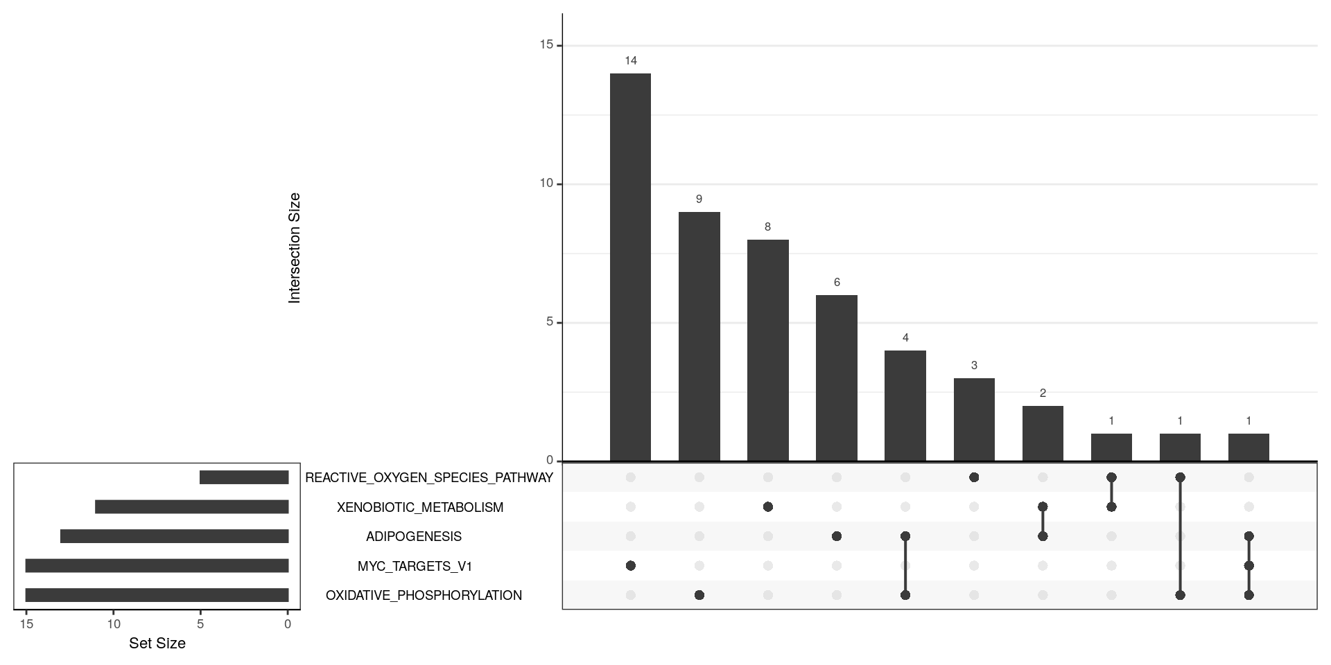
UpSet plot indicating distribution of DE genes within all significant terms from the HALLMARK gene sets. Most terms seem relatively independent of each other.
hmHeat <- hmMeta %>%
  dplyr::filter(nDE > 5, FDR < 0.05) %>%
  dplyr::select(gs_name, DE) %>%
  unnest(DE) %>%
  left_join(dgeList$genes, by = c("DE" = "gene_id")) %>%
  dplyr::select(gs_name, DE, gene_name) %>%
  mutate(belongs = TRUE) %>%
  pivot_wider(
    id_cols = c(DE, gene_name),
    names_from = gs_name,
    values_from = belongs,
    values_fill = list(belongs = FALSE)
  ) %>%
  left_join(
    cpm(fit$fitted.value, log = TRUE) %>%
      as.data.frame() %>%
      rownames_to_column("DE")
  )
hmHeat %>%
  dplyr::select(gene_name, starts_with("Ps")) %>%
  as.data.frame() %>%
  column_to_rownames("gene_name") %>%
  as.matrix() %>%
  pheatmap(
    color = viridis_pal(option = "magma")(100),
    legend_breaks = c(seq(-2, 8, by = 2), max(.)),
    legend_labels = c(seq(-2, 8, by = 2), "logCPM\n"),
    labels_col = hmHeat %>%
      dplyr::select(starts_with("Ps")) %>%
      colnames() %>%
      enframe(name = NULL) %>%
      dplyr::rename(sample = value) %>%
      left_join(dgeList$samples) %>%
      dplyr::select(sample, sampleID) %>%
      with(
        structure(sampleID, names = sample)
      ),
    cutree_rows = 6,
    cutree_cols = 3,
    annotation_names_row = FALSE,
    annotation_row = hmHeat %>%
      dplyr::select(gene_name, starts_with("HALLMARK_")) %>%
      mutate_at(vars(starts_with("HALL")), as.character) %>%
      as.data.frame() %>%
      column_to_rownames("gene_name") %>%
      set_colnames(
        str_remove(colnames(.), "HALLMARK_")
      )
  )
Gene expression patterns for all DE genes in HALLMARK genes sets, containing more than 5 DE genes.
KEGG Gene Sets
kgFry <- fit$fitted.values %>%
  cpm(log = TRUE) %>%
  fry(
    index = kgByID,
    design = fit$design,
    contrast = "mutant",
    sort = "directional"
    ) %>%
  rownames_to_column("gs_name") %>%
  as_tibble()
For analysis under camera when inter-gene correlations were calculated for a more conservative result.
kgCamera <- fit$fitted.values %>%
  cpm(log = TRUE) %>%
  camera(
    index = kgByID,
    design = fit$design,
    contrast = "mutant",
    inter.gene.cor = NULL
    ) %>%
  rownames_to_column("gs_name") %>%
  as_tibble()
For generation of the GSEA ranked list, 100,000 permutations were conducted.
kgGsea <- fgsea(
  pathways = kgByID,
  stats = rnk,
  nperm = np
) %>%
  as_tibble() %>%
  dplyr::rename(gs_name = pathway, PValue = pval) %>%
  arrange(PValue)
Results for all analyses, including goseq were then combined using Wilkinson’s method to combine p-values. For a conservative approach, under \(m\) tests, the \(m - 1^{\text{th}}\) smallest p-value was chosen.
kgMeta <- kgFry %>%
  dplyr::select(gs_name, fry = PValue) %>%
  left_join(
    dplyr::select(kgCamera, gs_name, camera = PValue)
  ) %>%
  left_join(
    dplyr::select(kgGsea, gs_name, gsea = PValue)
  ) %>%
  left_join(
    dplyr::select(kgRiboGoseq, gs_name, goseq = PValue)
  ) %>%
  nest(p = one_of(c("fry", "camera", "gsea", "goseq"))) %>%
  mutate(
    n_p = vapply(p, function(x){sum(!is.na(unlist(x)))}, integer(1)),
    wilkinson_p = vapply(p, function(x){
      x <- unlist(x)
      x <- x[!is.na(x)]
      wilkinsonp(x, length(x) - 1)$p
    }, numeric(1)),
    FDR = p.adjust(wilkinson_p, "fdr"),
    adjP = p.adjust(wilkinson_p, "bonferroni")
  ) %>%
  arrange(wilkinson_p) %>%
  unnest(p) %>%
  left_join(gsSizes) %>%
  mutate(
    DE = lapply(gene_id, intersect, dplyr::filter(deTable, DE)$gene_id),
    DE = lapply(DE, unique),
    nDE = vapply(DE, length, integer(1))
  )
kgMeta %>%
dplyr::filter(FDR < 0.05, nDE > 0) %>%
mutate_at(vars(one_of(c("wilkinson_p", "FDR", "adjP"))), formatP) %>%
dplyr::select(`Gene Set` = gs_name, `Number DE` = nDE, `Set Size` = gs_size, `Wilkinson~p~` = wilkinson_p, `p~FDR~` = FDR, `p~bonf~` = adjP) %>%
pander(
caption = "Results from combining all above approaches for the KEGG Gene Sets. All terms are significant to an FDR of 0.05. Only Gene Sets with at least one DE gene are shown.",
justify = "lrrrrr"
)| Gene Set | Number DE | Set Size | Wilkinsonp | pFDR | pbonf |
|---|---|---|---|---|---|
| KEGG_RIBOSOME | 26 | 80 | 5.11e-14 | 9.51e-12 | 9.51e-12 |
| KEGG_PRIMARY_IMMUNODEFICIENCY | 2 | 15 | 1.75e-05 | 0.0007 | 0.0033 |
| KEGG_OXIDATIVE_PHOSPHORYLATION | 14 | 119 | 3.59e-05 | 0.0010 | 0.0067 |
| KEGG_CYSTEINE_AND_METHIONINE_METABOLISM | 4 | 26 | 0.0001 | 0.0020 | 0.0189 |
| KEGG_ASTHMA | 1 | 3 | 0.0003 | 0.0038 | 0.0493 |
| KEGG_PARKINSONS_DISEASE | 13 | 112 | 0.0003 | 0.0038 | 0.0534 |
| KEGG_RETINOL_METABOLISM | 3 | 25 | 0.0005 | 0.0064 | 0.0960 |
| KEGG_GLUTATHIONE_METABOLISM | 4 | 36 | 0.0015 | 0.0150 | 0.2704 |
| KEGG_ALLOGRAFT_REJECTION | 1 | 4 | 0.0016 | 0.0156 | 0.2965 |
| KEGG_HUNTINGTONS_DISEASE | 15 | 159 | 0.0027 | 0.0227 | 0.5003 |
| KEGG_HEMATOPOIETIC_CELL_LINEAGE | 3 | 31 | 0.0047 | 0.0376 | 0.8812 |
| KEGG_METABOLISM_OF_XENOBIOTICS_BY_CYTOCHROME_P450 | 3 | 26 | 0.0048 | 0.0376 | 0.9014 |
| KEGG_RENIN_ANGIOTENSIN_SYSTEM | 1 | 8 | 0.0059 | 0.0430 | 1.0000 |
| KEGG_DRUG_METABOLISM_CYTOCHROME_P450 | 3 | 26 | 0.0060 | 0.0430 | 1.0000 |
| KEGG_SYSTEMIC_LUPUS_ERYTHEMATOSUS | 5 | 86 | 0.0065 | 0.0450 | 1.0000 |
kgMeta %>%
  dplyr::filter(nDE > 0, FDR < 0.05) %>%
  dplyr::select(gs_name, DE) %>%
  unnest(DE) %>%
  mutate(
    gs_name = str_remove(gs_name, "KEGG_"),
    gs_name = fct_lump(gs_name, n = 7)
    ) %>%
  split(f = .$gs_name) %>%
  lapply(magrittr::extract2, "DE") %>%
  fromList() %>%
  upset(
    nsets = length(.),
    order.by = "freq"
    )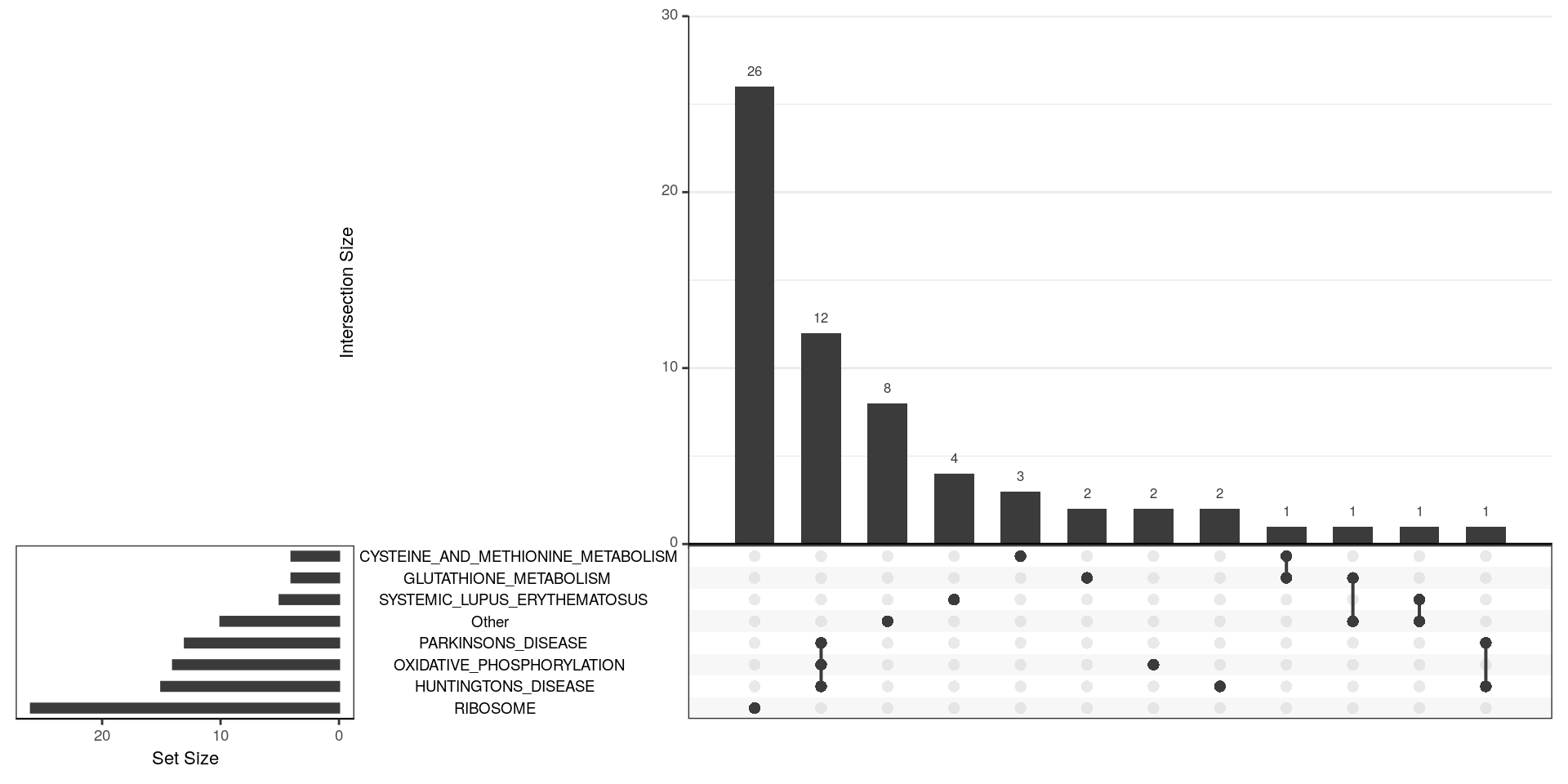
UpSet plot indicating distribution of DE genes within all significant terms from the KEGG gene sets. There is considerable overlap between Oxidative Phosphorylation and both Parkinson’s and Huntington’s Disease, indicating that these terms essentially capture the same signal.
riboOx <- kg %>%
  dplyr::filter(
    grepl("OXIDATIVE_PHOS", gs_name) | grepl("RIBOSOME", gs_name),
    gene_id %in% dplyr::filter(deTable, DE)$gene_id
    ) %>%
  mutate(gs_name = str_remove(gs_name, "(KEGG|HALLMARK)_")) %>%
  distinct(gs_name, gene_id) %>%
  left_join(
    cpm(fit$fitted.values, log = TRUE) %>%
      as.data.frame() %>%
      rownames_to_column("gene_id") %>%
      as_tibble()
    ) %>%
  pivot_longer(cols = starts_with("Ps"), names_to = "sample", values_to = "CPM") %>%
  left_join(dgeList$samples) %>%
  left_join(dgeList$genes) %>%
  dplyr::select(gs_name, gene_name, sampleID, genotype, CPM) %>%
  pivot_wider(
    id_cols = c(gs_name, gene_name),
    values_from = CPM,
    names_from = sampleID
  )
riboOx %>%
  dplyr::select(-gs_name) %>%
  as.data.frame() %>%
  column_to_rownames("gene_name") %>%
  as.matrix() %>%
  pheatmap(
    annotation_row = data.frame(
      GeneSet = riboOx$gs_name %>% str_replace("OXI.+", "OXPHOS"),
      row.names = riboOx$gene_name
      ),
    # annotation_col = tibble(
    #   sampleID = colnames(riboOx)[-c(1:2)]
    # ) %>%
    #   left_join(dgeList$samples) %>%
    #   dplyr::select(sampleID, Genotype = genotype) %>%
    #   as.data.frame() %>%
    #   column_to_rownames("sampleID"),
    color = viridis_pal(option = "magma")(100),
    legend_breaks = c(seq(-2, 8, by = 2), max(.)),
    legend_labels = c(seq(-2, 8, by = 2), "logCPM\n"),
    annotation_names_row = FALSE,
    cutree_rows = 5
  )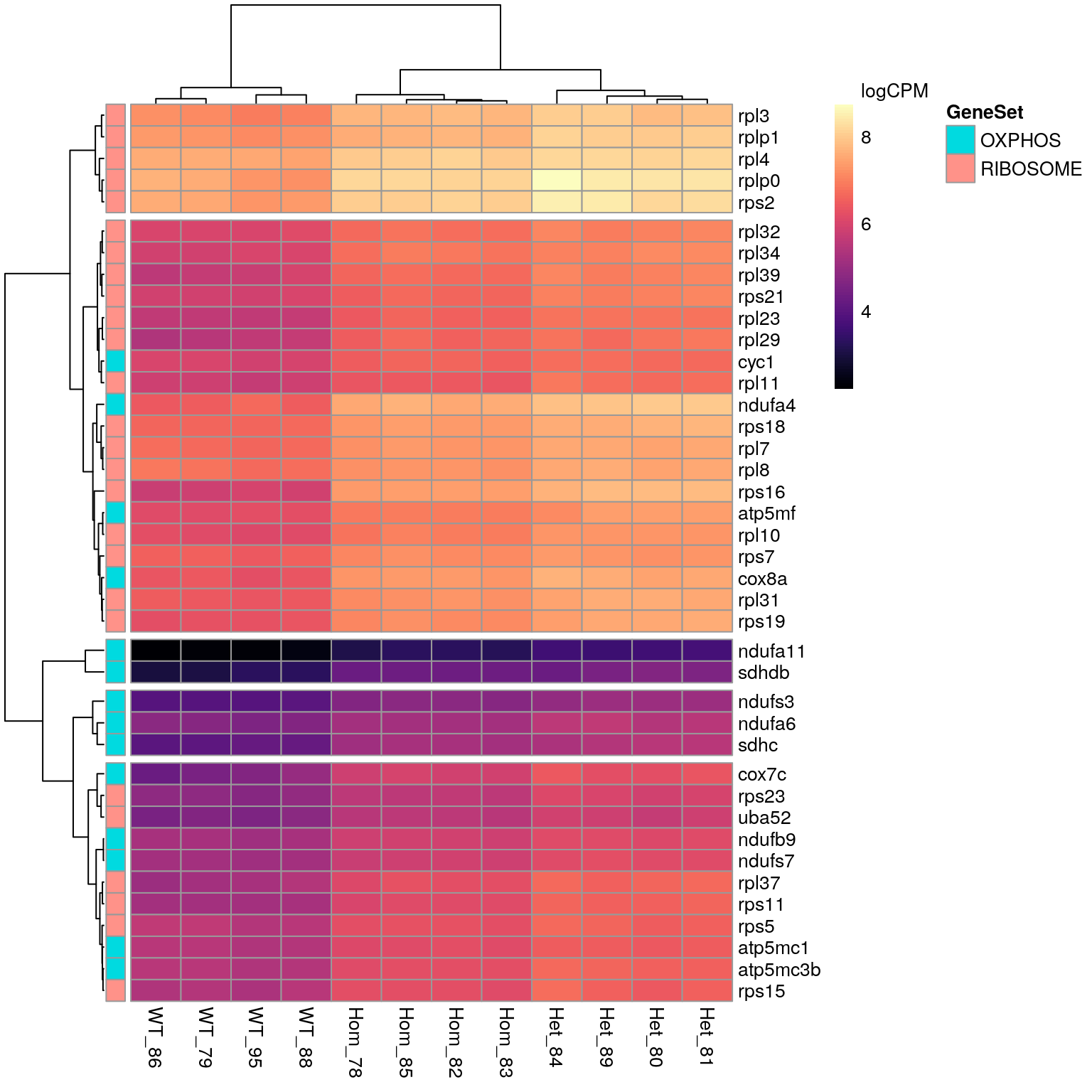
Given that the largest gene sets within the KEGG results were Oxidative Phosphorylation and Ribosomal gene sets, all DE genes associated with these KEGG terms are displayed below. All genes appear to show increased expression in mutant samples.
GO Gene Sets
goFry <- fit$fitted.values %>%
  cpm(log = TRUE) %>%
  fry(
    index = goByID,
    design = fit$design,
    contrast = "mutant",
    sort = "directional"
    ) %>%
  rownames_to_column("gs_name") %>%
  as_tibble()
For analysis under camera inter-gene correlations were directly calculated for a more conservative result.
goCamera <- fit$fitted.values %>%
  cpm(log = TRUE) %>%
  camera(
    index = goByID,
    design = fit$design,
    contrast = "mutant",
    inter.gene.cor = NULL
    ) %>%
  rownames_to_column("gs_name") %>%
  as_tibble()
For generation of the GSEA ranked list, 100,000 permutations were conducted.
goGsea <- fgsea(
  pathways = goByID,
  stats = rnk,
  nperm = np
) %>%
  as_tibble() %>%
  dplyr::rename(gs_name = pathway, PValue = pval) %>%
  arrange(PValue)
Results for all analyses, including goseq were then combined using Wilkinson’s method to combine p-values. For a conservative approach, under \(m\) tests, the \(m - 1^{\text{th}}\) smallest p-value was chosen.
goMeta <- goFry %>%
  dplyr::select(gs_name, fry = PValue) %>%
  left_join(
    dplyr::select(goCamera, gs_name, camera = PValue)
  ) %>%
  left_join(
    dplyr::select(goGsea, gs_name, gsea = PValue)
  ) %>%
  left_join(
    dplyr::select(goRiboGoseq, gs_name, goseq = PValue)
  )  %>%
  nest(p = one_of(c("fry", "camera", "gsea", "goseq"))) %>%
  mutate(
    n_p = vapply(p, function(x){sum(!is.na(unlist(x)))}, integer(1)),
    wilkinson_p = vapply(p, function(x){
      x <- unlist(x)
      x <- x[!is.na(x)]
      wilkinsonp(x, length(x) - 1)$p
    }, numeric(1)),
    FDR = p.adjust(wilkinson_p, "fdr"),
    adjP = p.adjust(wilkinson_p, "bonferroni")
  ) %>%
  arrange(wilkinson_p) %>%
   unnest(p) %>%
  left_join(gsSizes) %>%
  mutate(
    DE = lapply(gene_id, intersect, dplyr::filter(deTable, DE)$gene_id),
    DE = lapply(DE, unique),
    nDE = vapply(DE, length, integer(1))
  )
goMeta %>%
dplyr::filter(FDR < 0.01, nDE > 0) %>%
mutate_at(vars(one_of(c("wilkinson_p", "FDR", "adjP"))), formatP) %>%
mutate(gs_name = str_trunc(gs_name, 70)) %>%
dplyr::select(`Gene Set` = gs_name, `Number DE` = nDE, `Set Size` = gs_size, `Wilkinson~p~` = wilkinson_p, `p~FDR~` = FDR, `p~bonf~` = adjP) %>%
pander(
caption = "Results from combining all above approaches for the GO Gene Sets. All terms are significant using an FDR < 0.01. Only Gene Sets with at least one DE gene are shown.",
justify = "lrrrrr"
)| Gene Set | Number DE | Set Size | Wilkinsonp | pFDR | pbonf |
|---|---|---|---|---|---|
| GO_CYTOSOLIC_LARGE_RIBOSOMAL_SUBUNIT | 15 | 51 | 4.68e-14 | 5.23e-11 | 4.14e-10 |
| GO_COTRANSLATIONAL_PROTEIN_TARGETING_TO_MEMBRANE | 28 | 93 | 5.44e-14 | 5.23e-11 | 4.81e-10 |
| GO_CYTOSOLIC_RIBOSOME | 27 | 97 | 5.51e-14 | 5.23e-11 | 4.86e-10 |
| GO_ESTABLISHMENT_OF_PROTEIN_LOCALIZATION_TO_ENDOPLASMIC_RETICULUM | 27 | 105 | 5.60e-14 | 5.23e-11 | 4.95e-10 |
| GO_PROTEIN_LOCALIZATION_TO_ENDOPLASMIC_RETICULUM | 27 | 128 | 5.96e-14 | 5.23e-11 | 5.27e-10 |
| GO_PROTEIN_TARGETING_TO_MEMBRANE | 30 | 171 | 6.54e-14 | 5.23e-11 | 5.78e-10 |
| GO_VIRAL_GENE_EXPRESSION | 29 | 172 | 6.57e-14 | 5.23e-11 | 5.81e-10 |
| GO_RIBOSOMAL_SUBUNIT | 28 | 175 | 6.58e-14 | 5.23e-11 | 5.81e-10 |
| GO_TRANSLATIONAL_INITIATION | 29 | 177 | 6.61e-14 | 5.23e-11 | 5.84e-10 |
| GO_NUCLEAR_TRANSCRIBED_MRNA_CATABOLIC_PROCESS | 30 | 183 | 6.67e-14 | 5.23e-11 | 5.90e-10 |
| GO_CYTOSOLIC_PART | 30 | 206 | 7.06e-14 | 5.23e-11 | 6.24e-10 |
| GO_RIBOSOME | 30 | 210 | 7.10e-14 | 5.23e-11 | 6.27e-10 |
| GO_LARGE_RIBOSOMAL_SUBUNIT | 17 | 108 | 8.71e-12 | 5.92e-09 | 7.70e-08 |
| GO_RNA_CATABOLIC_PROCESS | 34 | 337 | 3.70e-11 | 2.33e-08 | 3.27e-07 |
| GO_ESTABLISHMENT_OF_PROTEIN_LOCALIZATION_TO_MEMBRANE | 30 | 287 | 4.55e-11 | 2.68e-08 | 4.02e-07 |
| GO_CYTOSOLIC_SMALL_RIBOSOMAL_SUBUNIT | 11 | 41 | 6.56e-11 | 3.62e-08 | 5.80e-07 |
| GO_PROTEIN_TARGETING | 34 | 379 | 2.20e-10 | 1.14e-07 | 1.94e-06 |
| GO_RRNA_BINDING | 11 | 57 | 3.48e-10 | 1.71e-07 | 3.07e-06 |
| GO_SYMPORTER_ACTIVITY | 10 | 94 | 5.13e-09 | 2.27e-06 | 4.53e-05 |
| GO_DRUG_TRANSMEMBRANE_TRANSPORTER_ACTIVITY | 8 | 76 | 1.08e-08 | 4.53e-06 | 9.52e-05 |
| GO_ORGANIC_ACID_TRANSMEMBRANE_TRANSPORTER_ACTIVITY | 9 | 105 | 1.81e-08 | 6.96e-06 | 0.0002 |
| GO_ORGANIC_ANION_TRANSMEMBRANE_TRANSPORTER_ACTIVITY | 11 | 144 | 2.33e-08 | 8.58e-06 | 0.0002 |
| GO_TRABECULA_FORMATION | 4 | 17 | 2.79e-08 | 9.86e-06 | 0.0002 |
| GO_ORGANIC_CYCLIC_COMPOUND_CATABOLIC_PROCESS | 40 | 474 | 3.73e-08 | 1.27e-05 | 0.0003 |
| GO_ESTABLISHMENT_OF_PROTEIN_LOCALIZATION_TO_ORGANELLE | 38 | 484 | 7.96e-08 | 2.60e-05 | 0.0007 |
| GO_ORGANIC_ACID_TRANSMEMBRANE_TRANSPORT | 9 | 106 | 8.97e-08 | 2.83e-05 | 0.0008 |
| GO_NEGATIVE_REGULATION_OF_INSULIN_SECRETION_INVOLVED_IN_CELLULAR_RE… | 3 | 9 | 1.55e-07 | 4.72e-05 | 0.0014 |
| GO_SECONDARY_ACTIVE_TRANSMEMBRANE_TRANSPORTER_ACTIVITY | 13 | 154 | 1.87e-07 | 5.50e-05 | 0.0016 |
| GO_RIBOSOME_ASSEMBLY | 9 | 57 | 1.97e-07 | 5.57e-05 | 0.0017 |
| GO_DRUG_TRANSMEMBRANE_TRANSPORT | 6 | 65 | 2.02e-07 | 5.57e-05 | 0.0018 |
| GO_POLYSOMAL_RIBOSOME | 7 | 28 | 2.58e-07 | 6.80e-05 | 0.0023 |
| GO_L_AMINO_ACID_TRANSMEMBRANE_TRANSPORTER_ACTIVITY | 4 | 44 | 2.62e-07 | 6.80e-05 | 0.0023 |
| GO_AEROBIC_ELECTRON_TRANSPORT_CHAIN | 3 | 19 | 2.99e-07 | 7.55e-05 | 0.0026 |
| GO_CYTOPLASMIC_TRANSLATION | 11 | 87 | 3.11e-07 | 7.64e-05 | 0.0028 |
| GO_INNER_MITOCHONDRIAL_MEMBRANE_PROTEIN_COMPLEX | 16 | 124 | 3.77e-07 | 9.01e-05 | 0.0033 |
| GO_SMALL_RIBOSOMAL_SUBUNIT | 11 | 69 | 3.93e-07 | 9.13e-05 | 0.0035 |
| GO_ACTIVE_TRANSMEMBRANE_TRANSPORTER_ACTIVITY | 15 | 254 | 4.19e-07 | 9.49e-05 | 0.0037 |
| GO_UBIQUITIN_LIGASE_INHIBITOR_ACTIVITY | 3 | 4 | 6.91e-07 | 0.0002 | 0.0061 |
| GO_AMINO_ACID_TRANSMEMBRANE_TRANSPORTER_ACTIVITY | 5 | 60 | 7.80e-07 | 0.0002 | 0.0069 |
| GO_PEPTIDE_BIOSYNTHETIC_PROCESS | 38 | 572 | 9.11e-07 | 0.0002 | 0.0081 |
| GO_ORGANIC_ACID_BIOSYNTHETIC_PROCESS | 12 | 198 | 1.63e-06 | 0.0003 | 0.0144 |
| GO_UBIQUITIN_PROTEIN_TRANSFERASE_INHIBITOR_ACTIVITY | 3 | 5 | 2.02e-06 | 0.0004 | 0.0178 |
| GO_RESPIRATORY_CHAIN_COMPLEX_IV | 2 | 14 | 2.15e-06 | 0.0004 | 0.0190 |
| GO_CELLULAR_AMIDE_METABOLIC_PROCESS | 45 | 805 | 3.20e-06 | 0.0006 | 0.0283 |
| GO_AMIDE_BIOSYNTHETIC_PROCESS | 40 | 678 | 3.83e-06 | 0.0007 | 0.0338 |
| GO_PLATELET_DENSE_GRANULE_LUMEN | 2 | 7 | 4.18e-06 | 0.0007 | 0.0369 |
| GO_ANION_TRANSMEMBRANE_TRANSPORTER_ACTIVITY | 17 | 228 | 4.28e-06 | 0.0007 | 0.0378 |
| GO_HEART_TRABECULA_FORMATION | 3 | 11 | 4.73e-06 | 0.0008 | 0.0418 |
| GO_PROSTANOID_BIOSYNTHETIC_PROCESS | 3 | 17 | 5.26e-06 | 0.0009 | 0.0464 |
| GO_ORGANIC_ACID_TRANSPORT | 14 | 240 | 5.61e-06 | 0.0009 | 0.0495 |
| GO_NEGATIVE_REGULATION_OF_UBIQUITIN_PROTEIN_LIGASE_ACTIVITY | 3 | 7 | 5.85e-06 | 0.0009 | 0.0517 |
| GO_POSITIVE_REGULATION_OF_SIGNAL_TRANSDUCTION_BY_P53_CLASS_MEDIATOR | 4 | 17 | 6.25e-06 | 0.0010 | 0.0552 |
| GO_REGULATION_OF_UBIQUITIN_PROTEIN_TRANSFERASE_ACTIVITY | 6 | 44 | 6.25e-06 | 0.0010 | 0.0553 |
| GO_DNA_METHYLATION_OR_DEMETHYLATION | 7 | 56 | 6.73e-06 | 0.0010 | 0.0595 |
| GO_PROTON_TRANSPORTING_ATP_SYNTHASE_COMPLEX | 4 | 20 | 8.60e-06 | 0.0012 | 0.0760 |
| GO_DRUG_CATABOLIC_PROCESS | 5 | 55 | 1.00e-05 | 0.0014 | 0.0883 |
| GO_DRUG_TRANSPORT | 8 | 152 | 1.05e-05 | 0.0015 | 0.0926 |
| GO_NEGATIVE_REGULATION_OF_SMOOTH_MUSCLE_CELL_DIFFERENTIATION | 3 | 14 | 1.28e-05 | 0.0017 | 0.1127 |
| GO_UBIQUITIN_PROTEIN_TRANSFERASE_REGULATOR_ACTIVITY | 5 | 13 | 1.28e-05 | 0.0017 | 0.1127 |
| GO_ANION_TRANSMEMBRANE_TRANSPORT | 15 | 203 | 1.31e-05 | 0.0017 | 0.1160 |
| GO_OXIDATIVE_PHOSPHORYLATION | 15 | 122 | 1.35e-05 | 0.0017 | 0.1189 |
| GO_NEGATIVE_REGULATION_OF_MACROPHAGE_CHEMOTAXIS | 2 | 2 | 1.78e-05 | 0.0022 | 0.1575 |
| GO_MONOCARBOXYLIC_ACID_TRANSMEMBRANE_TRANSPORTER_ACTIVITY | 3 | 28 | 1.85e-05 | 0.0023 | 0.1632 |
| GO_POSITIVE_REGULATION_OF_CYTOKINE_BIOSYNTHETIC_PROCESS | 3 | 28 | 2.10e-05 | 0.0025 | 0.1855 |
| GO_HIGH_DENSITY_LIPOPROTEIN_PARTICLE | 2 | 9 | 2.52e-05 | 0.0029 | 0.2224 |
| GO_SMALL_MOLECULE_BIOSYNTHETIC_PROCESS | 23 | 478 | 2.97e-05 | 0.0033 | 0.2622 |
| GO_FAT_SOLUBLE_VITAMIN_METABOLIC_PROCESS | 3 | 27 | 3.05e-05 | 0.0034 | 0.2698 |
| GO_POLYSOME | 8 | 65 | 3.25e-05 | 0.0035 | 0.2871 |
| GO_REGULATION_OF_INTRINSIC_APOPTOTIC_SIGNALING_PATHWAY_BY_P53_CLASS… | 4 | 21 | 3.65e-05 | 0.0038 | 0.3220 |
| GO_MACROLIDE_BINDING | 3 | 8 | 3.65e-05 | 0.0038 | 0.3225 |
| GO_REGULATION_OF_HISTONE_H3_K9_TRIMETHYLATION | 3 | 9 | 3.78e-05 | 0.0038 | 0.3343 |
| GO_ACYLGLYCEROL_TRANSPORT | 2 | 4 | 4.02e-05 | 0.0039 | 0.3553 |
| GO_ORGANIC_ANION_TRANSPORT | 16 | 345 | 4.19e-05 | 0.0041 | 0.3701 |
| GO_GENERATION_OF_PRECURSOR_METABOLITES_AND_ENERGY | 25 | 422 | 4.45e-05 | 0.0042 | 0.3931 |
| GO_ATP_SYNTHESIS_COUPLED_ELECTRON_TRANSPORT | 12 | 85 | 4.62e-05 | 0.0043 | 0.4078 |
| GO_RESPIRATORY_CHAIN_COMPLEX | 11 | 75 | 5.10e-05 | 0.0046 | 0.4508 |
| GO_REGULATION_OF_SYSTEMIC_ARTERIAL_BLOOD_PRESSURE_BY_CIRCULATORY_RE… | 2 | 8 | 5.24e-05 | 0.0046 | 0.4632 |
| GO_HETEROCHROMATIN | 7 | 66 | 5.32e-05 | 0.0046 | 0.4698 |
| GO_HUMORAL_IMMUNE_RESPONSE | 7 | 91 | 5.40e-05 | 0.0046 | 0.4769 |
| GO_ORGANONITROGEN_COMPOUND_BIOSYNTHETIC_PROCESS | 68 | 1,431 | 5.40e-05 | 0.0046 | 0.4771 |
| GO_RIBOSOMAL_LARGE_SUBUNIT_ASSEMBLY | 5 | 28 | 5.50e-05 | 0.0046 | 0.4856 |
| GO_PLASMINOGEN_ACTIVATION | 3 | 21 | 6.30e-05 | 0.0052 | 0.5564 |
| GO_NEGATIVE_REGULATION_OF_UBIQUITIN_PROTEIN_TRANSFERASE_ACTIVITY | 3 | 13 | 6.56e-05 | 0.0053 | 0.5796 |
| GO_ANTIBIOTIC_CATABOLIC_PROCESS | 4 | 25 | 7.09e-05 | 0.0056 | 0.6261 |
| GO_INHIBITORY_EXTRACELLULAR_LIGAND_GATED_ION_CHANNEL_ACTIVITY | 2 | 15 | 7.33e-05 | 0.0057 | 0.6480 |
| GO_NEGATIVE_REGULATION_OF_LEUKOCYTE_MIGRATION | 3 | 21 | 7.54e-05 | 0.0058 | 0.6657 |
| GO_ENERGY_DERIVATION_BY_OXIDATION_OF_ORGANIC_COMPOUNDS | 18 | 242 | 7.55e-05 | 0.0058 | 0.6666 |
| GO_ICOSANOID_BIOSYNTHETIC_PROCESS | 4 | 24 | 8.61e-05 | 0.0062 | 0.7606 |
| GO_POSITIVE_REGULATION_OF_INTRINSIC_APOPTOTIC_SIGNALING_PATHWAY_BY_… | 2 | 4 | 9.01e-05 | 0.0065 | 0.7957 |
| GO_REGULATION_OF_FATTY_ACID_BIOSYNTHETIC_PROCESS | 3 | 30 | 9.20e-05 | 0.0065 | 0.8130 |
| GO_REGULATION_OF_NUCLEOBASE_CONTAINING_COMPOUND_METABOLIC_PROCESS | 24 | 421 | 9.38e-05 | 0.0066 | 0.8286 |
| GO_POSITIVE_REGULATION_OF_INTERLEUKIN_2_BIOSYNTHETIC_PROCESS | 2 | 6 | 9.51e-05 | 0.0066 | 0.8398 |
| GO_NEGATIVE_REGULATION_OF_CHROMATIN_ORGANIZATION | 5 | 52 | 0.0001 | 0.0073 | 0.9565 |
| GO_INTERLEUKIN_2_BIOSYNTHETIC_PROCESS | 2 | 8 | 0.0001 | 0.0073 | 0.9576 |
| GO_AMINO_ACID_TRANSMEMBRANE_TRANSPORT | 5 | 69 | 0.0001 | 0.0073 | 0.9649 |
| GO_ANION_TRANSPORT | 22 | 434 | 0.0001 | 0.0074 | 1.0000 |
| GO_TETRAPYRROLE_BINDING | 5 | 61 | 0.0001 | 0.0074 | 1.0000 |
| GO_ACTIVIN_BINDING | 3 | 15 | 0.0001 | 0.0074 | 1.0000 |
| GO_E_BOX_BINDING | 4 | 41 | 0.0001 | 0.0074 | 1.0000 |
| GO_FIBRONECTIN_BINDING | 2 | 23 | 0.0001 | 0.0074 | 1.0000 |
| GO_NEGATIVE_REGULATION_OF_MITOCHONDRION_ORGANIZATION | 4 | 46 | 0.0001 | 0.0074 | 1.0000 |
| GO_DOUBLE_STRANDED_DNA_BINDING | 30 | 740 | 0.0001 | 0.0076 | 1.0000 |
| GO_REGULATION_OF_SYSTEMIC_ARTERIAL_BLOOD_PRESSURE_BY_RENIN_ANGIOTENSIN | 2 | 11 | 0.0001 | 0.0082 | 1.0000 |
| GO_PROTEIN_LOCALIZATION_TO_MEMBRANE | 35 | 539 | 0.0001 | 0.0082 | 1.0000 |
| GO_REGULATION_OF_INFLAMMATORY_RESPONSE_TO_ANTIGENIC_STIMULUS | 2 | 17 | 0.0001 | 0.0084 | 1.0000 |
| GO_DNA_METHYLATION | 5 | 44 | 0.0001 | 0.0085 | 1.0000 |
| GO_DNA_MODIFICATION | 7 | 75 | 0.0001 | 0.0085 | 1.0000 |
| GO_NEGATIVE_REGULATION_OF_TOLL_LIKE_RECEPTOR_SIGNALING_PATHWAY | 3 | 26 | 0.0001 | 0.0088 | 1.0000 |
| GO_NITRIC_OXIDE_MEDIATED_SIGNAL_TRANSDUCTION | 3 | 22 | 0.0002 | 0.0089 | 1.0000 |
| GO_RESPIRATORY_ELECTRON_TRANSPORT_CHAIN | 12 | 103 | 0.0002 | 0.0091 | 1.0000 |
| GO_ELECTRON_TRANSPORT_CHAIN | 14 | 153 | 0.0002 | 0.0098 | 1.0000 |
| GO_RIBOSOMAL_SMALL_SUBUNIT_ASSEMBLY | 3 | 16 | 0.0002 | 0.0098 | 1.0000 |
goMeta %>%
  dplyr::filter(nDE >= 25, FDR < 0.05) %>%
  dplyr::select(gs_name, DE) %>%
  unnest(DE) %>%
  mutate(
    gs_name = str_remove(gs_name, "GO_"),
    gs_name = fct_lump(gs_name, n = 12)
    ) %>%
  split(f = .$gs_name) %>%
  lapply(magrittr::extract2, "DE") %>%
  fromList() %>%
  upset(
    nsets = length(.),
    order.by = "freq",
    mb.ratio = c(0.55, 0.45)
  )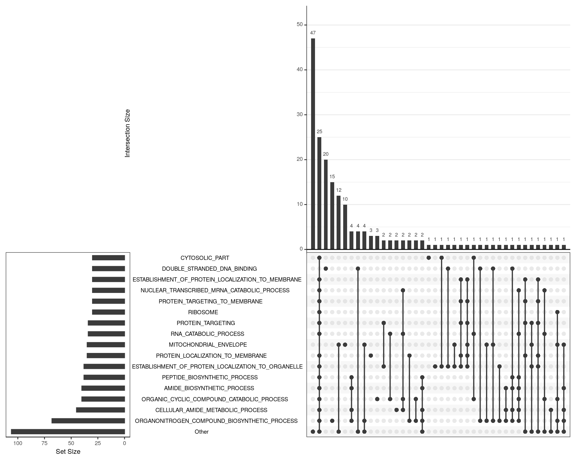
UpSet plot indicating distribution of DE genes within significant terms from the GO gene sets. Gene sets were restricted to those with 25 or more DE genes and an FDR < 0.05. A group of 47 genes is widely spread across multiple terms, whilst a group of 25 genes is shared by a large group of terms, indicating that these genes largely drive the signal for these terms. These genes tend to indicate Ribosomal activity. However, a set of 20 genes seems to more uniquely indicate dsDNA binding, whilst another 15 indicate organo-nitrogen biosynthesis, and a further set of 22 DE genes are predominantly associated with the mitochondrial envelope.
Genes Associated with dsDNA Binding
go %>%
  dplyr::filter(
    gs_name == "GO_DOUBLE_STRANDED_DNA_BINDING",
    gene_id %in% dplyr::filter(deTable, DE)$gene_id
  ) %>%
  dplyr::select(
    gene_id, gene_name
  ) %>%
  left_join(
    fit$fitted.values %>%
      cpm(log = TRUE) %>%
      as.data.frame() %>%
      rownames_to_column("gene_id")
  ) %>%
  dplyr::select(gene_name, starts_with("Ps")) %>%
  as.data.frame() %>%
  column_to_rownames("gene_name") %>%
  as.matrix() %>%
  pheatmap(
    color = viridis_pal(option = "magma")(100),
    legend_breaks = c(seq(-2, 8, by = 2), max(.)),
    legend_labels = c(seq(-2, 8, by = 2), "logCPM\n"),
    labels_col = hmHeat %>%
      dplyr::select(starts_with("Ps")) %>%
      colnames() %>%
      enframe(name = NULL) %>%
      dplyr::rename(sample = value) %>%
      left_join(dgeList$samples) %>%
      dplyr::select(sample, sampleID) %>%
      with(
        structure(sampleID, names = sample)
      ),
    cutree_rows = 4,
    cutree_cols = 3
  )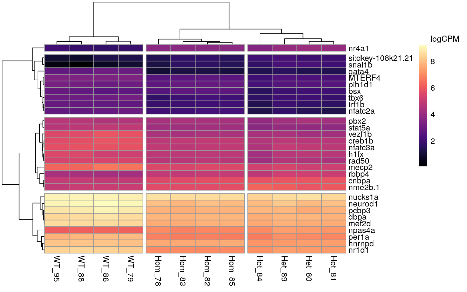
All DE genes associated with the GO term ‘Double Stranded DNA Binding’.
Genes Associated with the Mitochondrial Envelope
go %>%
  dplyr::filter(
    gs_name == "GO_MITOCHONDRIAL_ENVELOPE",
    gene_id %in% dplyr::filter(deTable, DE)$gene_id
  ) %>%
  dplyr::select(
    gene_id, gene_name
  ) %>%
  left_join(
    fit$fitted.values %>%
      cpm(log = TRUE) %>%
      as.data.frame() %>%
      rownames_to_column("gene_id")
  ) %>%
  dplyr::select(gene_name, starts_with("Ps")) %>%
  as.data.frame() %>%
  column_to_rownames("gene_name") %>%
  as.matrix() %>%
  pheatmap(
    color = viridis_pal(option = "magma")(100),
    legend_breaks = c(seq(-2, 8, by = 2), max(.)),
    legend_labels = c(seq(-2, 8, by = 2), "logCPM\n"),
    labels_col = hmHeat %>%
      dplyr::select(starts_with("Ps")) %>%
      colnames() %>%
      enframe(name = NULL) %>%
      dplyr::rename(sample = value) %>%
      left_join(dgeList$samples) %>%
      dplyr::select(sample, sampleID) %>%
      with(
        structure(sampleID, names = sample)
      ),
    cutree_rows = 4,
    cutree_cols = 3
  )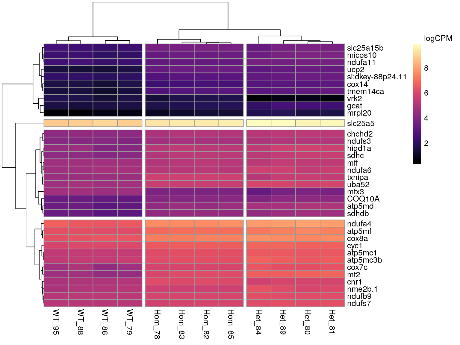
All DE genes associated with the GO term ‘Mitochondrial Envelope’.
Genes Associated with Organo-Nitrogen Compound Biosynthesis
go %>%
  dplyr::filter(
    gs_name %in% c(
      "GO_ORGANONITROGEN_COMPOUND_BIOSYNTHETIC_PROCESS", "GO_RIBOSOME"
    ),
    gene_id %in% dplyr::filter(deTable, DE)$gene_id
  ) %>%
  group_by(gene_id, gene_name) %>%
  tally() %>%
  ungroup() %>%
  dplyr::filter(n == 1) %>%
  dplyr::select(
    gene_id, gene_name
  ) %>%
  left_join(
    fit$fitted.values %>%
      cpm(log = TRUE) %>%
      as.data.frame() %>%
      rownames_to_column("gene_id")
  ) %>%
  dplyr::select(gene_name, starts_with("Ps")) %>%
  as.data.frame() %>%
  column_to_rownames("gene_name") %>%
  as.matrix() %>%
  pheatmap(
    color = viridis_pal(option = "magma")(100),
    legend_breaks = c(seq(-2, 8, by = 2), max(.)),
    legend_labels = c(seq(-2, 8, by = 2), "logCPM\n"),
    labels_col = hmHeat %>%
      dplyr::select(starts_with("Ps")) %>%
      colnames() %>%
      enframe(name = NULL) %>%
      dplyr::rename(sample = value) %>%
      left_join(dgeList$samples) %>%
      dplyr::select(sample, sampleID) %>%
      with(
        structure(sampleID, names = sample)
      ),
    cutree_rows = 4,
    cutree_cols = 3
  )
All DE genes associated with the GO term ‘Organo-Nitrogen Compound Biosynthetic Process’, excluding those genes which are additionally annotated to the GO term ‘Ribosome’.
Data Export
All enriched gene sets with an FDR adjusted p-value < 0.05 were exported as a single csv file.
bind_rows(
  hmMeta,
  kgMeta,
  goMeta
) %>%
  dplyr::filter(FDR < 0.05) %>%
  mutate(
    DE = lapply(DE, function(x){dplyr::filter(deTable, gene_id %in% x)$gene_name}),
    DE = lapply(DE, unique),
    DE = vapply(DE, paste, character(1), collapse = ";")
  ) %>%
  arrange(wilkinson_p) %>%
  dplyr::select(
    gs_name, gs_size, nDE, wilkinson_p, FDR, fry, camera, gsea, goseq, DE
  ) %>%
  write_csv(here::here("output", "Enrichment_Mutant_V_WT.csv"))
devtools::session_info()─ Session info ───────────────────────────────────────────────────────────────
setting value
version R version 3.6.2 (2019-12-12)
os Ubuntu 18.04.4 LTS
system x86_64, linux-gnu
ui X11
language en_AU:en
collate en_AU.UTF-8
ctype en_AU.UTF-8
tz Australia/Adelaide
date 2020-02-20
─ Packages ───────────────────────────────────────────────────────────────────
package * version date lib source
AnnotationDbi * 1.48.0 2019-10-29 [2] Bioconductor
askpass 1.1 2019-01-13 [2] CRAN (R 3.6.0)
assertthat 0.2.1 2019-03-21 [2] CRAN (R 3.6.0)
backports 1.1.5 2019-10-02 [2] CRAN (R 3.6.1)
BiasedUrn * 1.07 2015-12-28 [2] CRAN (R 3.6.1)
bibtex 0.4.2.2 2020-01-02 [2] CRAN (R 3.6.2)
Biobase * 2.46.0 2019-10-29 [2] Bioconductor
BiocFileCache 1.10.2 2019-11-08 [2] Bioconductor
BiocGenerics * 0.32.0 2019-10-29 [2] Bioconductor
BiocParallel 1.20.1 2019-12-21 [2] Bioconductor
biomaRt 2.42.0 2019-10-29 [2] Bioconductor
Biostrings 2.54.0 2019-10-29 [2] Bioconductor
bit 1.1-15.1 2020-01-14 [2] CRAN (R 3.6.2)
bit64 0.9-7 2017-05-08 [2] CRAN (R 3.6.0)
bitops 1.0-6 2013-08-17 [2] CRAN (R 3.6.0)
blob 1.2.1 2020-01-20 [2] CRAN (R 3.6.2)
broom 0.5.4 2020-01-27 [2] CRAN (R 3.6.2)
callr 3.4.1 2020-01-24 [2] CRAN (R 3.6.2)
cellranger 1.1.0 2016-07-27 [2] CRAN (R 3.6.0)
cli 2.0.1 2020-01-08 [2] CRAN (R 3.6.2)
cluster 2.1.0 2019-06-19 [2] CRAN (R 3.6.1)
codetools 0.2-16 2018-12-24 [4] CRAN (R 3.6.0)
colorspace 1.4-1 2019-03-18 [2] CRAN (R 3.6.0)
crayon 1.3.4 2017-09-16 [2] CRAN (R 3.6.0)
curl 4.3 2019-12-02 [2] CRAN (R 3.6.2)
data.table 1.12.8 2019-12-09 [2] CRAN (R 3.6.2)
DBI 1.1.0 2019-12-15 [2] CRAN (R 3.6.2)
dbplyr 1.4.2 2019-06-17 [2] CRAN (R 3.6.0)
DelayedArray 0.12.2 2020-01-06 [2] Bioconductor
desc 1.2.0 2018-05-01 [2] CRAN (R 3.6.0)
devtools 2.2.1 2019-09-24 [2] CRAN (R 3.6.1)
digest 0.6.23 2019-11-23 [2] CRAN (R 3.6.1)
dplyr * 0.8.4 2020-01-31 [2] CRAN (R 3.6.2)
edgeR * 3.28.0 2019-10-29 [2] Bioconductor
ellipsis 0.3.0 2019-09-20 [2] CRAN (R 3.6.1)
evaluate 0.14 2019-05-28 [2] CRAN (R 3.6.0)
FactoMineR 2.1 2020-01-17 [2] CRAN (R 3.6.2)
fansi 0.4.1 2020-01-08 [2] CRAN (R 3.6.2)
farver 2.0.3 2020-01-16 [2] CRAN (R 3.6.2)
fastmatch 1.1-0 2017-01-28 [2] CRAN (R 3.6.0)
fgsea * 1.12.0 2019-10-29 [2] Bioconductor
flashClust 1.01-2 2012-08-21 [2] CRAN (R 3.6.1)
forcats * 0.4.0 2019-02-17 [2] CRAN (R 3.6.0)
fs 1.3.1 2019-05-06 [2] CRAN (R 3.6.0)
gbRd 0.4-11 2012-10-01 [2] CRAN (R 3.6.0)
geneLenDataBase * 1.22.0 2019-11-05 [2] Bioconductor
generics 0.0.2 2018-11-29 [2] CRAN (R 3.6.0)
GenomeInfoDb 1.22.0 2019-10-29 [2] Bioconductor
GenomeInfoDbData 1.2.2 2019-11-21 [2] Bioconductor
GenomicAlignments 1.22.1 2019-11-12 [2] Bioconductor
GenomicFeatures 1.38.1 2020-01-22 [2] Bioconductor
GenomicRanges 1.38.0 2019-10-29 [2] Bioconductor
ggdendro 0.1-20 2016-04-27 [2] CRAN (R 3.6.0)
ggplot2 * 3.2.1 2019-08-10 [2] CRAN (R 3.6.1)
ggrepel 0.8.1 2019-05-07 [2] CRAN (R 3.6.0)
git2r 0.26.1 2019-06-29 [2] CRAN (R 3.6.1)
glue 1.3.1 2019-03-12 [2] CRAN (R 3.6.0)
GO.db 3.10.0 2019-11-21 [2] Bioconductor
goseq * 1.38.0 2019-10-29 [2] Bioconductor
gridExtra 2.3 2017-09-09 [2] CRAN (R 3.6.0)
gtable 0.3.0 2019-03-25 [2] CRAN (R 3.6.0)
haven 2.2.0 2019-11-08 [2] CRAN (R 3.6.1)
here 0.1 2017-05-28 [2] CRAN (R 3.6.0)
highr 0.8 2019-03-20 [2] CRAN (R 3.6.0)
hms 0.5.3 2020-01-08 [2] CRAN (R 3.6.2)
htmltools 0.4.0 2019-10-04 [2] CRAN (R 3.6.1)
htmlwidgets 1.5.1 2019-10-08 [2] CRAN (R 3.6.1)
httpuv 1.5.2 2019-09-11 [2] CRAN (R 3.6.1)
httr 1.4.1 2019-08-05 [2] CRAN (R 3.6.1)
hwriter 1.3.2 2014-09-10 [2] CRAN (R 3.6.0)
IRanges * 2.20.2 2020-01-13 [2] Bioconductor
jpeg 0.1-8.1 2019-10-24 [2] CRAN (R 3.6.1)
jsonlite 1.6 2018-12-07 [2] CRAN (R 3.6.0)
kableExtra 1.1.0 2019-03-16 [2] CRAN (R 3.6.1)
knitr 1.27 2020-01-16 [2] CRAN (R 3.6.2)
labeling 0.3 2014-08-23 [2] CRAN (R 3.6.0)
later 1.0.0 2019-10-04 [2] CRAN (R 3.6.1)
lattice 0.20-38 2018-11-04 [4] CRAN (R 3.6.0)
latticeExtra 0.6-29 2019-12-19 [2] CRAN (R 3.6.2)
lazyeval 0.2.2 2019-03-15 [2] CRAN (R 3.6.0)
leaps 3.1 2020-01-16 [2] CRAN (R 3.6.2)
lifecycle 0.1.0 2019-08-01 [2] CRAN (R 3.6.1)
limma * 3.42.1 2020-01-29 [2] Bioconductor
locfit 1.5-9.1 2013-04-20 [2] CRAN (R 3.6.0)
lubridate 1.7.4 2018-04-11 [2] CRAN (R 3.6.0)
magrittr * 1.5 2014-11-22 [2] CRAN (R 3.6.0)
MASS 7.3-51.5 2019-12-20 [4] CRAN (R 3.6.2)
Matrix 1.2-18 2019-11-27 [2] CRAN (R 3.6.1)
matrixStats 0.55.0 2019-09-07 [2] CRAN (R 3.6.1)
memoise 1.1.0 2017-04-21 [2] CRAN (R 3.6.0)
metap * 1.3 2020-01-23 [2] CRAN (R 3.6.2)
mgcv 1.8-31 2019-11-09 [4] CRAN (R 3.6.1)
mnormt 1.5-5 2016-10-15 [2] CRAN (R 3.6.1)
modelr 0.1.5 2019-08-08 [2] CRAN (R 3.6.1)
msigdbr * 7.0.1 2019-09-04 [2] CRAN (R 3.6.2)
multcomp 1.4-12 2020-01-10 [2] CRAN (R 3.6.2)
multtest 2.42.0 2019-10-29 [2] Bioconductor
munsell 0.5.0 2018-06-12 [2] CRAN (R 3.6.0)
mutoss 0.1-12 2017-12-04 [2] CRAN (R 3.6.2)
mvtnorm 1.0-12 2020-01-09 [2] CRAN (R 3.6.2)
ngsReports * 1.1.2 2019-10-16 [1] Bioconductor
nlme 3.1-144 2020-02-06 [4] CRAN (R 3.6.2)
numDeriv 2016.8-1.1 2019-06-06 [2] CRAN (R 3.6.2)
openssl 1.4.1 2019-07-18 [2] CRAN (R 3.6.1)
pander * 0.6.3 2018-11-06 [2] CRAN (R 3.6.0)
pheatmap * 1.0.12 2019-01-04 [2] CRAN (R 3.6.0)
pillar 1.4.3 2019-12-20 [2] CRAN (R 3.6.2)
pkgbuild 1.0.6 2019-10-09 [2] CRAN (R 3.6.1)
pkgconfig 2.0.3 2019-09-22 [2] CRAN (R 3.6.1)
pkgload 1.0.2 2018-10-29 [2] CRAN (R 3.6.0)
plotly 4.9.1 2019-11-07 [2] CRAN (R 3.6.1)
plotrix 3.7-7 2019-12-05 [2] CRAN (R 3.6.2)
plyr 1.8.5 2019-12-10 [2] CRAN (R 3.6.2)
png 0.1-7 2013-12-03 [2] CRAN (R 3.6.0)
prettyunits 1.1.1 2020-01-24 [2] CRAN (R 3.6.2)
processx 3.4.1 2019-07-18 [2] CRAN (R 3.6.1)
progress 1.2.2 2019-05-16 [2] CRAN (R 3.6.0)
promises 1.1.0 2019-10-04 [2] CRAN (R 3.6.1)
ps 1.3.0 2018-12-21 [2] CRAN (R 3.6.0)
purrr * 0.3.3 2019-10-18 [2] CRAN (R 3.6.1)
R6 2.4.1 2019-11-12 [2] CRAN (R 3.6.1)
rappdirs 0.3.1 2016-03-28 [2] CRAN (R 3.6.0)
RColorBrewer * 1.1-2 2014-12-07 [2] CRAN (R 3.6.0)
Rcpp * 1.0.3 2019-11-08 [2] CRAN (R 3.6.1)
RCurl 1.98-1.1 2020-01-19 [2] CRAN (R 3.6.2)
Rdpack 0.11-1 2019-12-14 [2] CRAN (R 3.6.2)
readr * 1.3.1 2018-12-21 [2] CRAN (R 3.6.0)
readxl 1.3.1 2019-03-13 [2] CRAN (R 3.6.0)
remotes 2.1.0 2019-06-24 [2] CRAN (R 3.6.0)
reprex 0.3.0 2019-05-16 [2] CRAN (R 3.6.0)
reshape2 1.4.3 2017-12-11 [2] CRAN (R 3.6.0)
rlang 0.4.4 2020-01-28 [2] CRAN (R 3.6.2)
rmarkdown 2.1 2020-01-20 [2] CRAN (R 3.6.2)
rprojroot 1.3-2 2018-01-03 [2] CRAN (R 3.6.0)
Rsamtools 2.2.1 2019-11-06 [2] Bioconductor
RSQLite 2.2.0 2020-01-07 [2] CRAN (R 3.6.2)
rstudioapi 0.10 2019-03-19 [2] CRAN (R 3.6.0)
rtracklayer 1.46.0 2019-10-29 [2] Bioconductor
rvest 0.3.5 2019-11-08 [2] CRAN (R 3.6.1)
S4Vectors * 0.24.3 2020-01-18 [2] Bioconductor
sandwich 2.5-1 2019-04-06 [2] CRAN (R 3.6.1)
scales * 1.1.0 2019-11-18 [2] CRAN (R 3.6.1)
scatterplot3d 0.3-41 2018-03-14 [2] CRAN (R 3.6.1)
sessioninfo 1.1.1 2018-11-05 [2] CRAN (R 3.6.0)
ShortRead 1.44.1 2019-12-19 [2] Bioconductor
sn 1.5-5 2020-01-30 [2] CRAN (R 3.6.2)
statmod 1.4.33 2020-01-10 [2] CRAN (R 3.6.2)
stringi 1.4.5 2020-01-11 [2] CRAN (R 3.6.2)
stringr * 1.4.0 2019-02-10 [2] CRAN (R 3.6.0)
SummarizedExperiment 1.16.1 2019-12-19 [2] Bioconductor
survival 3.1-8 2019-12-03 [2] CRAN (R 3.6.2)
testthat 2.3.1 2019-12-01 [2] CRAN (R 3.6.1)
TFisher 0.2.0 2018-03-21 [2] CRAN (R 3.6.2)
TH.data 1.0-10 2019-01-21 [2] CRAN (R 3.6.1)
tibble * 2.1.3 2019-06-06 [2] CRAN (R 3.6.0)
tidyr * 1.0.2 2020-01-24 [2] CRAN (R 3.6.2)
tidyselect 1.0.0 2020-01-27 [2] CRAN (R 3.6.2)
tidyverse * 1.3.0 2019-11-21 [2] CRAN (R 3.6.1)
truncnorm 1.0-8 2018-02-27 [2] CRAN (R 3.6.0)
UpSetR * 1.4.0 2019-05-22 [2] CRAN (R 3.6.0)
usethis 1.5.1 2019-07-04 [2] CRAN (R 3.6.1)
vctrs 0.2.2 2020-01-24 [2] CRAN (R 3.6.2)
viridisLite 0.3.0 2018-02-01 [2] CRAN (R 3.6.0)
webshot 0.5.2 2019-11-22 [2] CRAN (R 3.6.1)
whisker 0.4 2019-08-28 [2] CRAN (R 3.6.1)
withr 2.1.2 2018-03-15 [2] CRAN (R 3.6.0)
workflowr * 1.6.0 2019-12-19 [2] CRAN (R 3.6.2)
xfun 0.12 2020-01-13 [2] CRAN (R 3.6.2)
XML 3.99-0.3 2020-01-20 [2] CRAN (R 3.6.2)
xml2 1.2.2 2019-08-09 [2] CRAN (R 3.6.1)
XVector 0.26.0 2019-10-29 [2] Bioconductor
yaml 2.2.1 2020-02-01 [2] CRAN (R 3.6.2)
zlibbioc 1.32.0 2019-10-29 [2] Bioconductor
zoo 1.8-7 2020-01-10 [2] CRAN (R 3.6.2)
[1] /home/steveped/R/x86_64-pc-linux-gnu-library/3.6
[2] /usr/local/lib/R/site-library
[3] /usr/lib/R/site-library
[4] /usr/lib/R/library