Phenotype Analysis of Brazilian Drought Trials

Last updated: 2022-11-10

Checks: 6 1

Knit directory: Genomic-Selection-for-Drought-Tolerance-Using-Genome-Wide-SNPs-in-Casava/

This reproducible R Markdown analysis was created with workflowr (version 1.7.0). The Checks tab describes the reproducibility checks that were applied when the results were created. The Past versions tab lists the development history.

R Markdown file: uncommitted changes

The R Markdown file has staged changes. To know which version of the R Markdown file created these results, you’ll want to first commit it to the Git repo. If you’re still working on the analysis, you can ignore this warning. When you’re finished, you can run wflow_publish to commit the R Markdown file and build the HTML.

Environment: empty

Great job! The global environment was empty. Objects defined in the global environment can affect the analysis in your R Markdown file in unknown ways. For reproduciblity it’s best to always run the code in an empty environment.

Seed: set.seed(20221020)

The command set.seed(20221020) was run prior to running the code in the R Markdown file. Setting a seed ensures that any results that rely on randomness, e.g. subsampling or permutations, are reproducible.

Session information: recorded

Great job! Recording the operating system, R version, and package versions is critical for reproducibility.

Cache: none

Nice! There were no cached chunks for this analysis, so you can be confident that you successfully produced the results during this run.

File paths: relative

Great job! Using relative paths to the files within your workflowr project makes it easier to run your code on other machines.

Repository version: b78c842

Great! You are using Git for version control. Tracking code development and connecting the code version to the results is critical for reproducibility.

The results in this page were generated with repository version b78c842. See the Past versions tab to see a history of the changes made to the R Markdown and HTML files.

Note that you need to be careful to ensure that all relevant files for the analysis have been committed to Git prior to generating the results (you can use wflow_publish or wflow_git_commit). workflowr only checks the R Markdown file, but you know if there are other scripts or data files that it depends on. Below is the status of the Git repository when the results were generated:


Ignored files:
    Ignored:    .Rproj.user/

Untracked files:
    Untracked:  data/AllGBSandDArTClones_ReadyForGP_Dos.rds
    Untracked:  data/DCas22_GBSandDArT_ReadyForGP_Dos.rds
    Untracked:  data/allchrAR08.txt
    Untracked:  data/convet_haplo_diplo.txt
    Untracked:  output/BLUPS.RDS
    Untracked:  output/BLUPS.csv
    Untracked:  output/BLUPS_par.Rdata
    Untracked:  output/herdabilidade.csv
    Untracked:  output/media_pheno.csv
    Untracked:  output/resultMM.Rdata

Unstaged changes:
    Deleted:    BLUPS.RDS
    Deleted:    BLUPS.csv
    Deleted:    BLUPs.Rdata
    Deleted:    RR-BLUP-method.pdf
    Modified:   analysis/GWS.Rmd
    Modified:   analysis/phenotype.Rmd
    Deleted:    cor-methods-RR_BLUP.pdf
    Deleted:    deregress.Rdata
    Deleted:    geno.txt
    Deleted:    geno2.txt
    Deleted:    herdabilidade.csv

Staged changes:
    New:        BLUPS.RDS
    New:        BLUPS.csv
    New:        BLUPs.Rdata
    New:        RR-BLUP-method.pdf
    New:        analysis/GWS.Rmd
    Modified:   analysis/_site.yml
    Modified:   analysis/about.Rmd
    Modified:   analysis/index.Rmd
    Modified:   analysis/license.Rmd
    New:        analysis/phenotype.Rmd
    New:        cor-methods-RR_BLUP.pdf
    New:        data/Fenótipos Desregressados GBS Todos.RDS
    New:        data/Genomic Selection for Drought Tolerance Using Genome-Wide SNPs in Maize.pdf
    New:        data/Phenotyping v2.xlsx
    New:        data/Phenotyping.xlsx
    New:        data/SNPs.rds
    New:        data/deregress.Rdata
    New:        data/geno.rds
    New:        data/geno.txt
    New:        deregress.Rdata
    New:        geno.txt
    New:        geno2.txt
    New:        herdabilidade.csv

Note that any generated files, e.g. HTML, png, CSS, etc., are not included in this status report because it is ok for generated content to have uncommitted changes.

There are no past versions. Publish this analysis with wflow_publish() to start tracking its development.

Data and libraries

Load Libraries

library(kableExtra)
library(tidyverse)
require(ComplexHeatmap)
library(data.table)
library(readxl)
library(metan)
library(DataExplorer)
library(doParallel)
theme_set(theme_bw())

Data import and manipulation

Vamos importar o conjunto de dados fenotípicos, excluindo as variaveis sem informações e as variaveis Local (redundante com Ano) e Tratamento (só uma observação).

pheno <- read_excel("data/Phenotyping.xlsx",
                    na = "NA") %>%
  select_if( ~ !all(is.na(.))) %>%  # Deleting traits without information 
  select(-c("Local", "Tratamento"))

Vamos realizar alguma manipulações para ajustar nosso banco de dados e para facilitar a visualização da análise exploratória.

Primeiro, vamos converter as variaveis que são caracter em fatores. Depois vamos converter as variaveis que são referentes as notas para inteiro e logo em seguida em fatores. Após isso, vamos criar a variável ANo.Bloco para o aninhamento no modelo para obtenção dos BLUPs.

pheno <- pheno %>%
  mutate_if(is.character, as.factor) %>%
  mutate_at(c("RF", "Ácaro", "Vigor", "Branching_Level"), as.integer) %>%
  mutate_if(is.integer, as.factor) %>%
  mutate_at(
    c(
      "Ano",
      "Bloco",
      "Porte",
      "Incidence_Mites",
      "Stand_Final",
      "Staygreen",
      "Flowering"
    ),
    as.factor
  ) %>% # Convert Ano and Bloco, and traits in factors
  mutate(Ano.Bloco = factor(interaction(Ano, Bloco)))   # Convert Ano.Bloco interaction in factors

Exploratory Data Analysis

Análise introdutória de todo conjunto de dados

introduce(pheno) %>% 
  kbl(escape = F, align = 'c') %>%
  kable_classic(
    "hover",
    full_width = F,
    position = "center",
    fixed_thead = T
  )

rows	columns	discrete_columns	continuous_columns	all_missing_columns	total_missing_values	complete_rows	total_observations	memory_usage
2336	28	13	15	0	16771	440	65408	449920

Não temos nenhuma coluna que tenha todas observações ausentes, mas temos muitos valores ausentes em todo conjunto de dados. Algumas manipulações deverão ser realizadas para melhorar a qualidade dos dados.

Analise de Ano

Vamos produzir um heatmap para verificar a quantidade de clone em cada ano. Vou criar outro conjunto de dados com a contagem de Ano e Clone. Depois vou criar os objetos correspondentes à matriz de clones e de anos. Por fim, criei a matriz que representa a presença e ausencia do clone no ano.

pheno2 <- pheno %>%
  count(Ano, Clone)

genmat <- model.matrix(~ -1 + Clone, data = pheno2)
envmat <- model.matrix(~ -1 + Ano, data = pheno2)
genenvmat <- t(envmat) %*% genmat
genenvmat_ch <- ifelse(genenvmat == 1, "Present", "Abscent")

Heatmap(
  genenvmat_ch,
  col = c("white", "tomato"),
  show_column_names = F,
  heatmap_legend_param = list(title = ""),
  column_title = "Genotypes",
  row_title = "Environments"
)

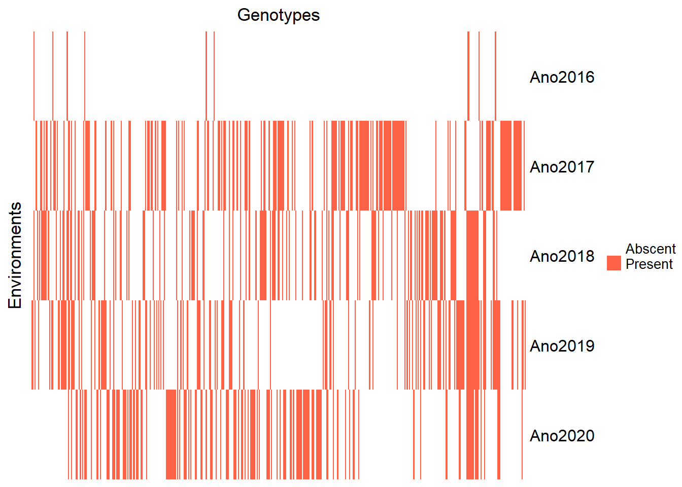
Pelo heatmap, fica claro que o ano 2016 possui muitas poucas observações. Então, devemos eliminá-lo.

pheno <- pheno %>% 
  filter(Ano != 2016) %>% 
  droplevels()

Apenas para conferência, vamos visualizar novamente o heatmap de clones por ano.

pheno2<- pheno %>% 
  count(Ano, Clone)
  
genmat = model.matrix( ~ -1 + Clone, data = pheno2)
envmat = model.matrix( ~ -1 + Ano, data = pheno2)
genenvmat = t(envmat) %*% genmat
genenvmat_ch = ifelse(genenvmat == 1, "Present", "Abscent")

Heatmap(
  genenvmat_ch,
  col = c("white", "tomato"),
  show_column_names = F,
  heatmap_legend_param = list(title = ""),
  column_title = "Genotypes",
  row_title = "Environments"
)

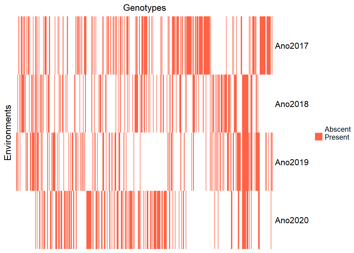
Aqui, é possível obervar que nosso conjunto de dados possui clones que foram avaliados em apenas um ano. Vamos visualizar isso, para verificarmos quantos clones foram avaliados de acordo com o número de anos.

pheno2 %>%
  count(Clone) %>%
  count(n) %>%
  kbl(
    escape = F,
    align = 'c',
    col.names = c("N of Environments", "Number of genotypes")
  ) %>%
  kable_classic(
    "hover",
    full_width = F,
    position = "center",
    fixed_thead = T
  )

Storing counts in `nn`, as `n` already present in input
i Use `name = "new_name"` to pick a new name.

N of Environments	Number of genotypes
1	350
2	72
3	20
4	5

Apenas 5 clones foram avaliados em todos os anos, isso possivelmente diminuirá nossa acurácia do modelos.

Além disso, observe que os anos diferem quanto ao número de clones avaliados:

pheno2 %>%
  group_by(Ano) %>%
  summarise(length(Clone)) %>%
  kbl(
    escape = F,
    align = 'c',
    col.names = c("Environments", "Number of genotypes")) %>%
  kable_classic(
    "hover",
    full_width = F,
    position = "center",
    fixed_thead = T
  )

Environments	Number of genotypes
2017	165
2018	138
2019	133
2020	138

Outro fator que diminui a acurácia, e por isso adotar modelos mistos na análise é o mais indicado para a obtenção dos BLUPS.

Podemos verificar quantos clones temos em comum entre os anos:

genenvmat %*% t(genenvmat) %>% 
  kbl(escape = F, align = 'c') %>%
  kable_classic(
    "hover",
    full_width = F,
    position = "center",
    fixed_thead = T
  )

	Ano2017	Ano2018	Ano2019	Ano2020
Ano2017	165	42	22	14
Ano2018	42	138	39	16
Ano2019	22	39	133	29
Ano2020	14	16	29	138

O ano 2020 apresenta menor número de clones em comum, no entanto, vamos mantê-lo para realizar as análises.

Análise das variáveis

Agora, iremos analisar a frequência para cada característica discreta.

plot_bar(pheno)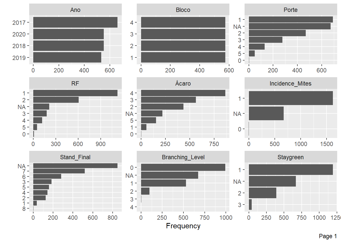

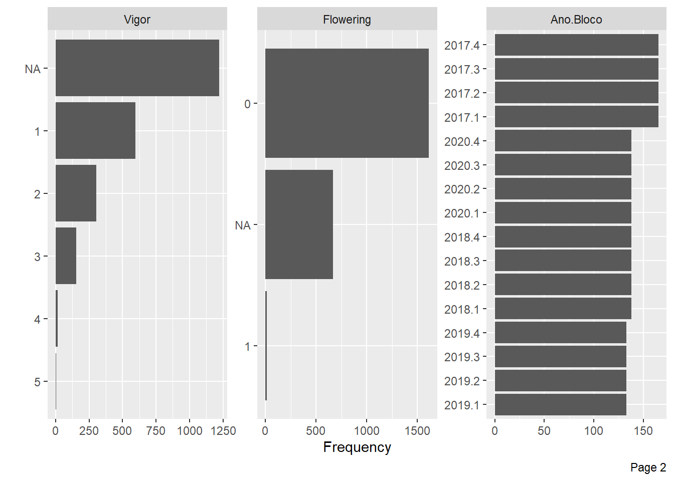
A Incidencia de ácaros e Florescimento possuem poucas informações para alguns níveis e muitos NA’s, também vamos excluir essas variáveis.

pheno <- pheno  %>% 
  select(-c(Incidence_Mites, Flowering))

plot_bar(pheno)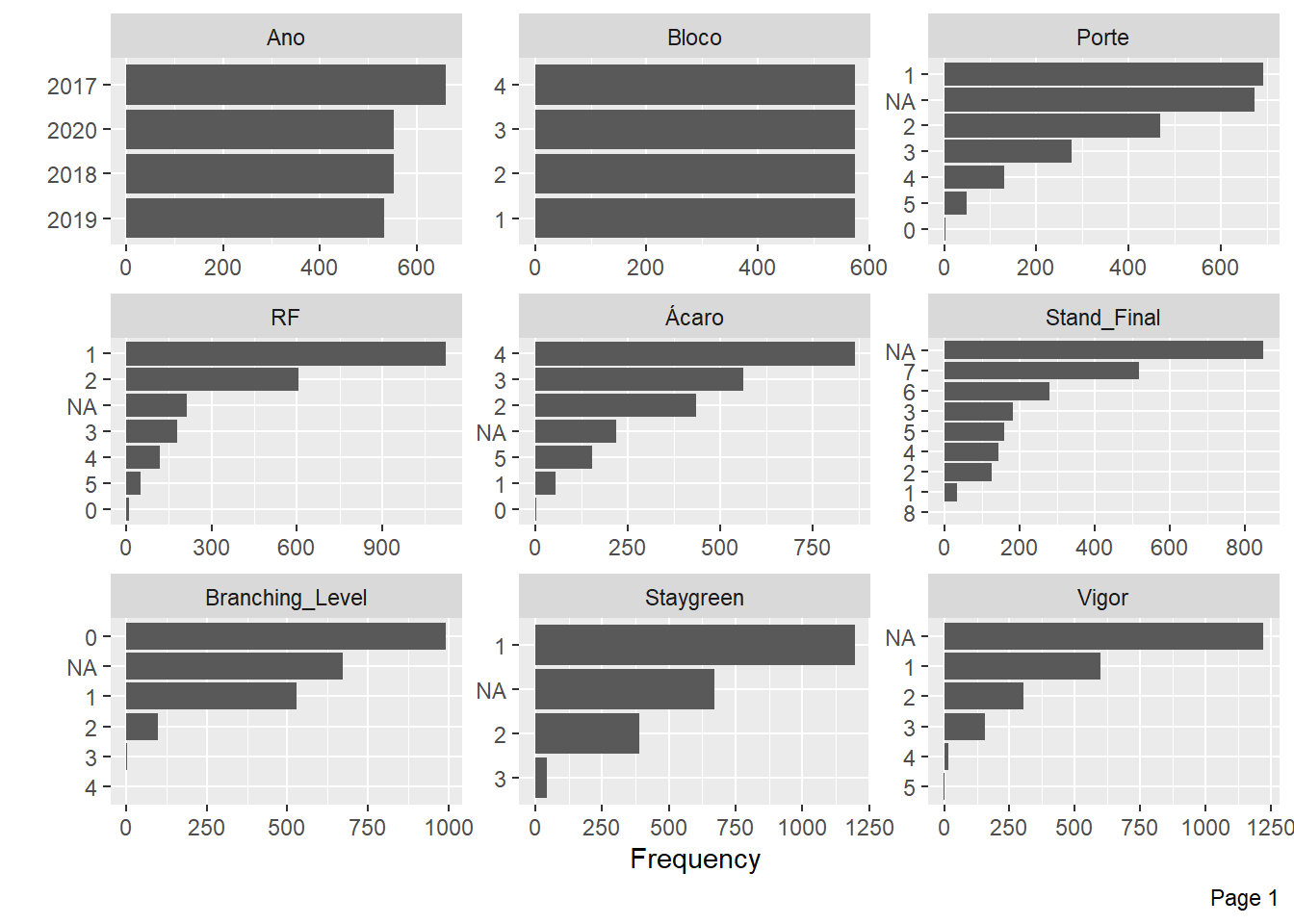

Vamos observar apenas os valores ausentes agora, para verificar as proporções.

plot_missing(pheno)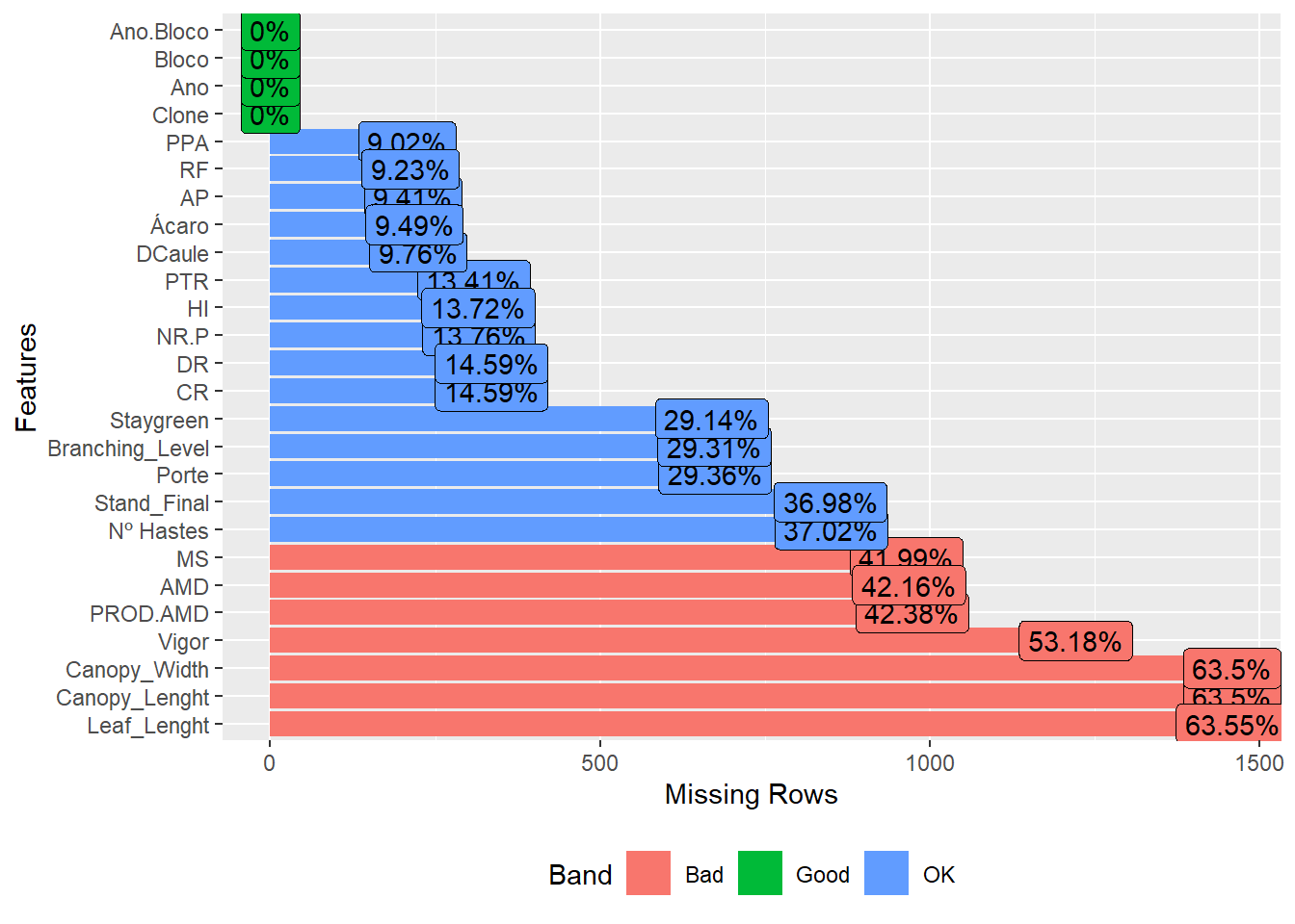

Temos uma proporção alta de valor ausente para Vigor, Leaf_Lenght, Canopy_Width e Canopy_Lenght, também vou excluir-lás.

pheno <- pheno %>% 
  select(-c(Vigor, Leaf_Lenght, Canopy_Width, Canopy_Lenght))

Vamos verificar a distribuição das características por ano agora.

plot_bar(pheno, by = "Ano")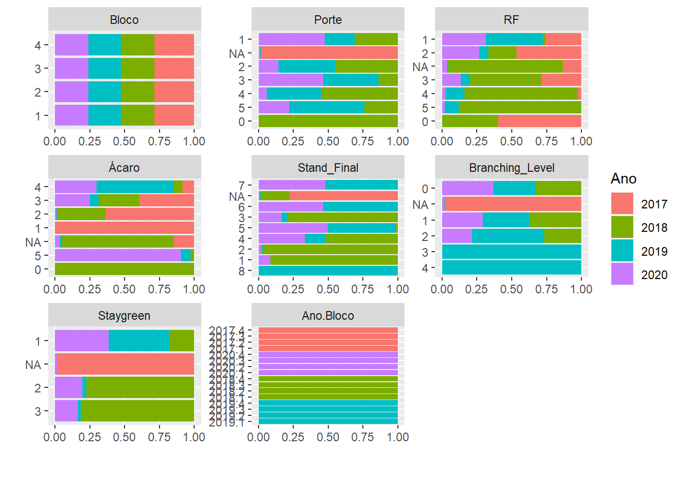

Para Porte, Branching_Level e Staygreen temos muitos valores ausentes para o ano de 2017, possivelmente não houve avaliação nesse ano para essas características. Para obter os BLUPs, teremos que remover esse Ano do banco de dados.

Agora vamos observar os histogramas das varaiveis quantitativas:

plot_histogram(pheno)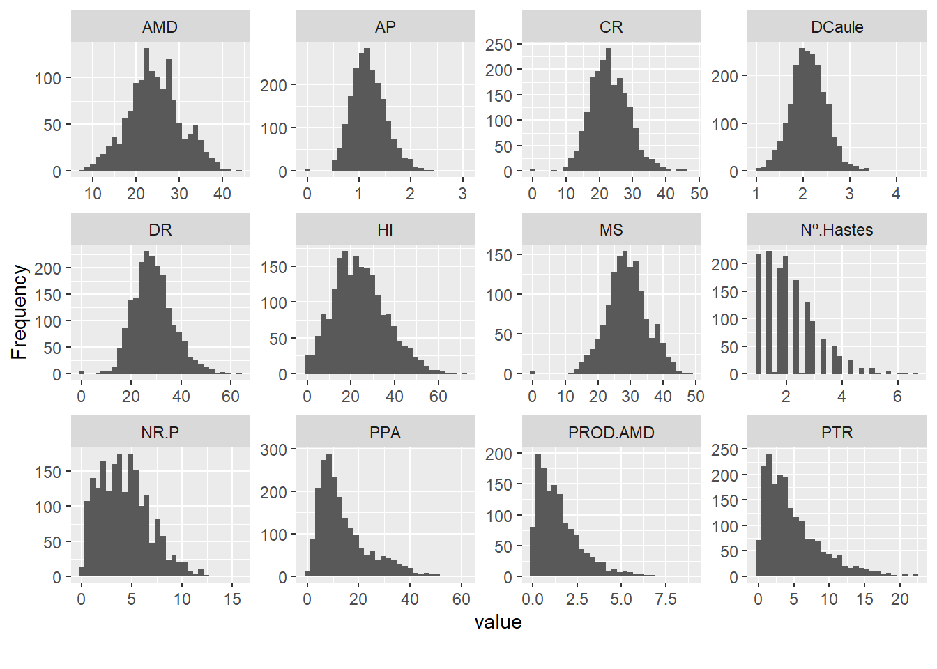

Vimos aqui que as variáveis quantitativas apresentam correlações entre si, principalmente entre PROD.AMD com PTR e AMD com MS

Vamos avaliar as estatisticas descritivas da combinação entre clone e ano para as variaveis.

ge_details(pheno, Ano, Clone, resp = everything()) %>% kbl(escape = F, align = 'c') %>%
  kable_classic(
    "hover",
    full_width = F,
    position = "center",
    fixed_thead = T
  )

Parameters	NR.P	PTR	PPA	MS	PROD.AMD	AP	HI	AMD	CR	DR	DCaule	Nº Hastes
Mean	4.28	4.88	14.2	28.97	1.51	1.19	24.23	24.42	23.17	28.82	2.11	2.13
SE	0.06	0.09	0.22	0.17	0.04	0.01	0.27	0.17	0.13	0.18	0.01	0.03
SD	2.52	4.06	10.17	6.29	1.27	0.33	12.13	6.11	5.89	7.99	0.38	0.95
CV	58.9	83.19	71.66	21.73	84.4	27.81	50.08	25.05	25.42	27.75	17.9	44.53
Min	0 (BGM-0019 in 2019)	0 (BGM-0019 in 2019)	0 (BGM-0044 in 2018)	0 (BGM-0044 in 2018)	0 (BGM-0044 in 2018)	0 (BGM-0044 in 2018)	0 (BGM-0019 in 2019)	7.33 (BGM-0626 in 2020)	0 (BGM-0044 in 2018)	0 (BGM-0044 in 2018)	1.01 (BGM-0592 in 2018)	1 (BGM-0036 in 2018)
Max	15.67 (2012-107-002 in 2019)	22.2 (BGM-1267 in 2018)	61.17 (BGM-2124 in 2020)	48.34 (BGM-1015 in 2020)	8.87 (BGM-0396 in 2018)	3.03 (BR-11-24-156 in 2020)	71.97 (BGM-1315 in 2018)	43.69 (BGM-1015 in 2020)	47.33 (BGM-0396 in 2018)	63.3 (BRS Mulatinha in 2018)	4.37 (BRS Tapioqueira in 2020)	6.67 (BGM-0714 in 2019)
MinENV	2018 (1.6)	2017 (2.75)	2017 (8.47)	2020 (26.21)	2019 (1.32)	2017 (1)	2020 (18.61)	2020 (21.56)	2017 (19.72)	2017 (24.49)	2018 (2.02)	2018 (1.44)
MaxENV	2019 (5.74)	2020 (6.52)	2020 (25.87)	2018 (34.91)	2018 (1.81)	2019 (1.48)	2018 (31.84)	2018 (30.78)	2019 (27.14)	2018 (34.28)	2017 (2.16)	2019 (2.71)
MinGEN	BGM-0044 (0)	BGM-0044 (0)	BGM-0044 (0)	BGM-0044 (0)	BGM-0044 (0)	BGM-0044 (0)	BGM-0044 (0)	BGM-0626 (10.33)	BGM-0044 (0)	BGM-0044 (0)	BGM-0048 (1.25)	BGM-0066 (1)
MaxGEN	2012-107-002 (11.33)	IAC-14 (14.07)	BGM-2124 (54.33)	BGM-1015 (45.02)	BGM-1023 (4.76)	BGM-1200 (1.91)	Mata_Fome_Branca (52.78)	BGM-1015 (40.37)	BGM-1956 (35.5)	BGM-1956 (48.91)	BGM-1523 (2.93)	BGM-0451 (4.44)

O genótipo BGM-0044 apresentou valores nulos para a maioria das características, como foi avaliado apenas no ano de 2018, é melhor excluí-lo.

pheno<- pheno %>% 
  filter(Clone != "BGM-0044")%>% 
  droplevels()

Aparentemente não temos mais um genótipo que possa prejudicar nossa análise. Agora devemos avaliar as estatisticas descritivas apenas de clone para as variaveis.

desc_stat(pheno, by = Ano) %>%
  kbl(escape = F, align = 'c') %>%
  kable_classic(
    "hover",
    full_width = F,
    position = "center",
    fixed_thead = T
  )

Ano	variable	cv	max	mean	median	min	sd.amo	se	ci.t	n.valid
2017	AMD	NA	-Inf	NaN	NA	Inf	0.0000	NA	NaN	0
2017	AP	21.0398	1.6767	1.0023	1.0000	0.4500	0.2109	0.0084	0.0165	632
2017	CR	21.5823	31.6667	19.7236	19.6667	7.0000	4.2568	0.1719	0.3376	613
2017	DCaule	16.7774	3.3333	2.1581	2.1667	1.2000	0.3621	0.0144	0.0284	629
2017	DR	21.0039	39.6900	24.4889	24.4733	8.9867	5.1436	0.2077	0.4080	613
2017	HI	48.2942	66.6827	23.5691	22.7255	1.5744	11.3825	0.4612	0.9058	609
2017	MS	NA	-Inf	NaN	NA	Inf	0.0000	NA	NaN	0
2017	Nº Hastes	NA	-Inf	NaN	NA	Inf	0.0000	NA	NaN	0
2017	NR.P	48.8708	12.0000	4.3530	4.3330	0.1250	2.1273	0.0860	0.1689	612
2017	PPA	45.4973	22.2220	8.4677	8.0750	0.6940	3.8526	0.1542	0.3029	624
2017	PROD.AMD	NA	-Inf	NaN	NA	Inf	0.0000	NA	NaN	0
2017	PTR	66.8379	9.6700	2.7517	2.4310	0.1160	1.8392	0.0743	0.1459	613
2018	AMD	15.6937	41.4284	30.7820	31.3500	13.5318	4.8309	0.2794	0.5498	299
2018	AP	28.0409	1.9967	1.0953	1.0600	0.4867	0.3071	0.0159	0.0313	373
2018	CR	27.1625	47.3333	23.6102	23.0000	9.5000	6.4131	0.3715	0.7311	298
2018	DCaule	22.3814	3.7317	2.0189	1.9800	1.0133	0.4519	0.0235	0.0463	369
2018	DR	23.3943	63.3033	34.7356	34.4400	14.1300	8.1262	0.4707	0.9264	298
2018	HI	42.0024	71.9673	32.2503	32.6091	0.0000	13.5459	0.7719	1.5188	308
2018	MS	13.6086	46.0784	35.3819	36.0000	18.1818	4.8150	0.2785	0.5480	299
2018	Nº Hastes	33.4885	3.3333	1.4379	1.3333	1.0000	0.4815	0.0249	0.0490	373
2018	NR.P	63.2913	6.2500	1.6249	1.4085	0.1900	1.0284	0.0588	0.1157	306
2018	PPA	69.0625	31.6000	8.7610	7.2000	1.0000	6.0506	0.3022	0.5940	401
2018	PROD.AMD	91.8742	8.8669	1.8356	1.3539	0.0839	1.6864	0.0984	0.1936	294
2018	PTR	86.6619	22.2000	5.6274	4.2500	0.0000	4.8768	0.2770	0.5450	310
2019	AMD	16.5407	35.9441	23.6326	23.6328	10.7346	3.9090	0.1745	0.3428	502
2019	AP	19.1125	2.4233	1.4843	1.4633	0.7400	0.2837	0.0123	0.0243	528
2019	CR	21.1089	45.6667	27.1361	27.0000	11.0000	5.7281	0.2529	0.4969	513
2019	DCaule	15.7037	3.3203	2.1061	2.0963	1.1197	0.3307	0.0144	0.0283	528
2019	DR	24.3155	58.9267	33.4940	33.6500	6.1200	8.1442	0.3596	0.7064	513
2019	HI	47.3227	60.1626	26.1706	26.6117	0.0000	12.3846	0.5390	1.0588	528
2019	MS	13.8212	40.5941	28.2826	28.2828	15.3846	3.9090	0.1745	0.3428	502
2019	Nº Hastes	37.3740	6.6667	2.7113	2.6667	1.0000	1.0133	0.0441	0.0867	527
2019	NR.P	47.7261	15.6670	5.7402	5.6670	0.0000	2.7396	0.1192	0.2342	528
2019	PPA	47.4901	47.5710	13.4607	12.7735	1.2860	6.3925	0.2782	0.5465	528
2019	PROD.AMD	72.5347	5.4021	1.3211	1.1082	0.0000	0.9583	0.0428	0.0841	501
2019	PTR	74.3122	22.2000	5.2850	4.5000	0.0000	3.9274	0.1709	0.3358	528
2020	AMD	27.3600	43.6860	21.5594	21.3900	7.3260	5.8986	0.2569	0.5048	527
2020	AP	24.0927	3.0333	1.1945	1.1600	0.3600	0.2878	0.0124	0.0243	543
2020	CR	18.9730	36.6667	23.2345	23.3333	9.0000	4.4083	0.1909	0.3751	533
2020	DCaule	17.5042	4.3733	2.1321	2.1207	1.0547	0.3732	0.0160	0.0315	543
2020	DR	20.5858	43.2733	26.2101	26.1800	11.8533	5.3956	0.2337	0.4591	533
2020	HI	43.3204	45.9340	18.6129	18.0486	1.9608	8.0632	0.3496	0.6867	532
2020	MS	22.5059	48.3360	26.2094	26.0400	11.9760	5.8986	0.2569	0.5048	527
2020	Nº Hastes	37.1507	4.6667	2.0463	2.0000	1.0000	0.7602	0.0326	0.0641	543
2020	NR.P	47.0839	10.3330	4.3060	4.3330	0.3330	2.0274	0.0881	0.1730	530
2020	PPA	42.7475	61.1670	25.8653	25.9165	3.3330	11.0568	0.4794	0.9417	532
2020	PROD.AMD	81.2220	6.0724	1.5211	1.2326	0.0483	1.2354	0.0540	0.1060	524
2020	PTR	68.4455	20.5670	6.5246	5.9000	0.4000	4.4658	0.1934	0.3800	533

Novamente, algumas variáveis não foram computadas para o ano de 2017 então temos que eliminar esse ano na hora de realizar a análise para essas variaveis.

O que chama atenção nessa tabela são os cv altos para algumas característica, especialmente: HI, Nº de Hastes, NR.P, PPA, PROD.AMD e PTR.

Isso pode se dá devido a presença de outliers, vamos fazer uma inspeção em todo conjunto de dados para avaliar se há outliers:

inspect(pheno %>%
          select(-c(Clone)), verbose = FALSE) %>% kbl(escape = F, align = 'c') %>%
  kable_classic(
    "hover",
    full_width = F,
    position = "center",
    fixed_thead = T
  )

Variable	Class	Missing	Levels	Valid_n	Min	Median	Max	Outlier	Text
Ano	factor	No	4	2292	NA	NA	NA	NA	NA
Bloco	factor	No	4	2292	NA	NA	NA	NA	NA
NR.P	numeric	Yes		1976	0.00	4.00	15.67	16	NA
PTR	numeric	Yes		1984	0.00	3.70	22.20	76	NA
PPA	numeric	Yes		2085	0.69	11.17	61.17	89	NA
MS	numeric	Yes		1328	11.98	28.80	48.34	6	NA
PROD.AMD	numeric	Yes		1319	0.00	1.21	8.87	49	NA
AP	numeric	Yes		2076	0.36	1.16	3.03	23	NA
HI	numeric	Yes		1977	0.00	23.21	71.97	14	NA
AMD	numeric	Yes		1328	7.33	24.15	43.69	6	NA
Porte	factor	Yes	5	1618	NA	NA	NA	NA	NA
RF	factor	Yes	6	2080	NA	NA	NA	NA	NA
CR	numeric	Yes		1957	7.00	23.00	47.33	19	NA
DR	numeric	Yes		1957	6.12	28.17	63.30	32	NA
DCaule	numeric	Yes		2069	1.01	2.10	4.37	22	NA
Ácaro	factor	Yes	5	2074	NA	NA	NA	NA	NA
Nº Hastes	numeric	Yes		1443	1.00	2.00	6.67	30	NA
Stand_Final	factor	Yes	8	1444	NA	NA	NA	NA	NA
Branching_Level	factor	Yes	5	1619	NA	NA	NA	NA	NA
Staygreen	factor	Yes	3	1623	NA	NA	NA	NA	NA
Ano.Bloco	factor	No	16	2292	NA	NA	NA	NA	NA

Confirmando o que foi descrito antes, a maioria das variáveis com alto cv apresenta muitos outliers e por isso iremos excluir elas no loop para obtenção dos blups.

Geral Inspection

Agora vamos realizar apenas uma inspeção geral dos dados para finalizar as manipulações.

corr_plot(pheno, col.by = Ano)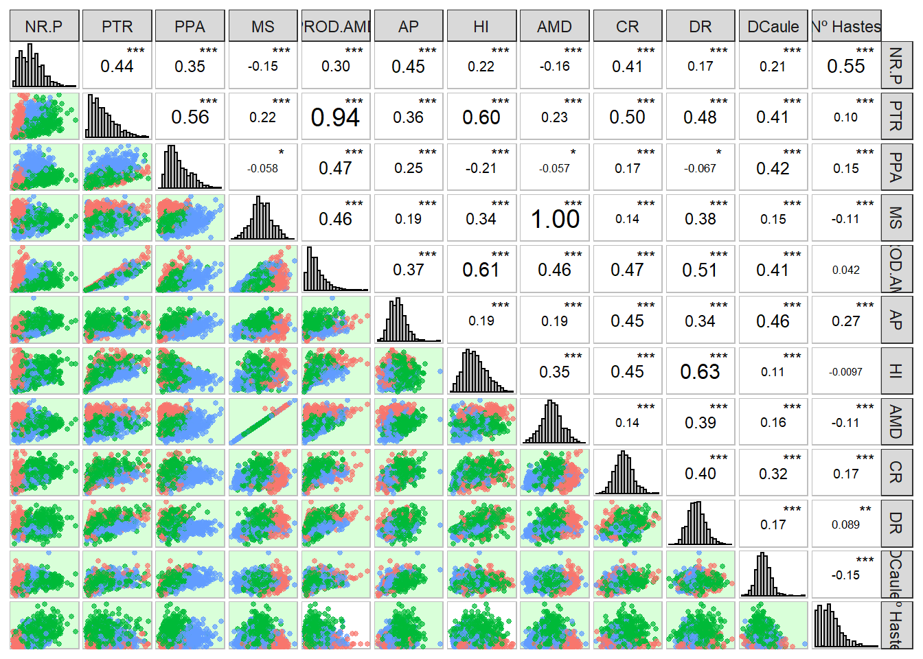

Amido com MS e PROD.AMD com PTR apresentam alta correlação.

Além disso a maioria das variáveis aparentemente apresentação distribuição normal dos dados fenotípicos. Dessa forma, vamos prosseguir para a obtenção dos blups.

Genotype-environment analysis by mixed-effect models

Primeiro, vou criar uma função para obter os blups e alguns parâmetros do nosso modelo.

BLUPS_par <- function(model, trait) {
  BLUP <- ranef(model, condVar = TRUE)$Clone
  PEV <-
    c(attr(BLUP, "postVar")) # PEV is a vector of error variances associated with each individual BLUP... # it tells you about how confident you should be in the estimate of an individual CLONE's BLUP value.
  Clone.var <-
    c(VarCorr(model)$Clone) # Extract the variance component for CLONE
  ResidVar <-
    (attr(VarCorr(model), "sc")) ^ 2 # Extract the residual variance component
  Ano <-
    c(VarCorr(model)$Ano) # Extract the variance component for Ano.Bloco
  Ano.Bloco <-
    c(VarCorr(model)$Ano.Bloco) # Extract the variance component for Ano.Bloco
  # You will need a line like the one above for every random effect (not for fixed effects)
  out <-
    BLUP / (1 - (PEV / Clone.var)) # This is the actual de-regress part (the BLUP for CLONE is divided by (1 - PEV/CLONE.var))
  r2 <-
    1 - (PEV / Clone.var) # Reliability: a confidence value for a BLUP (0 to 1 scale)
  H2 = Clone.var / (Clone.var + Ano.Bloco + ResidVar) # An estimate of the broad-sense heritability, must change this formula when you change the model analysis
  wt = (1 - H2) / ((0.1 + (1 - r2) / r2) * H2) # Weights for each de-regressed BLUP
  # There is a paper the determined this crazy formula, Garrick et al. 2009. I wouldn't pay much attn. to it.
  # These weights will be used in the second-step (e.g. cross-validation) to account for what we've done in this step
  # The weights will be fit as error variances associated with each residual value
  VarComps <- as.data.frame(VarCorr(model))
  
  return(
    list(
      Trait = trait,
      drgBLUP = out,
      BLUP = BLUP,
      weights = wt,
      varcomps = VarComps,
      H2 = H2,
      Reliability = r2,
      model = model
    )
  )
}

save(BLUPS_par, file = "output/BLUPS_par.Rdata")

The BLUP model

Aqui temos que lembrar que possuímos outliers para algumas características e também que devemos excluir o ano 2017 para algumas.

Vou criar um loop onde informo quais características onde esse ano deverá ser excluído e também utilizar a função de remover outliers.

As características que devemos excluir o ano 2017 são Porte, Branching_Level, Staygreen, AMD, MS, Nº Hastes e PROD.AMD.

excluir_2017 <- c("Porte", "Branching_Level", "Staygreen", "AMD", "MS", "Nº Hastes" , "PROD.AMD")

Usaremos esse vetor dentro do loop para exclusão do ano 2017 para essas variáveis.

Vamos converter todas as variáveis para numéricas agora.

traits <- colnames(pheno)[4:21]
pheno<- pheno %>% 
  mutate_at(traits, as.numeric)

Agora vamos realizar a análise de modelos mistos para obter os blups.

load("output/BLUPS_par.Rdata")

registerDoParallel(cores = 6) # Specify the number of cores (my lab computer has 8; I will use 6 of them)

resultMM <- foreach(a = traits, i = icount(), .inorder = TRUE) %dopar% {
  require(lme4)
  require(dplyr)
  library(purrr)
  
  # Loop para exclusão do ano 2017 de acordo com o vetor com os nomes da variáveis descritos anteriormente.
  if (a %in% excluir_2017) {
    data <- pheno %>%
      filter(Ano != 2017) %>%
      droplevels()
  } else{
    data <- pheno
  }
  
  # Exclusão dos primeiros outliers encontrados
  outliers <- boxplot(data[i+3], plot = FALSE)$out
  
  if(!is_empty(outliers)){
  data <- filter(data,data[i+3] != outliers)
  }
  
  model <- lmer(data = data,
                formula = get(traits[i]) ~ (1 |Clone) + Ano + (1|Ano.Bloco)) # Clone and Ano.Bloco are random and Ano is fixed
  
  
  result <- BLUPS_par(model, traits[i])
}

save(resultMM, file = "output/resultMM.Rdata")

BLUPS for `Clone`

Como usei “foreach” para executar cada análise do estágio 1 em paralelo, cada característica está em um elemento separado de uma lista Precisamos processar o objeto resultMM em um data.frame ou matriz para análise posterior.

load("output/resultMM.Rdata")

BLUPS <-
  data.frame(Clone = unique(pheno$Clone), stringsAsFactors = F)

H2 <- data.frame(H2 = "H2",
                 stringsAsFactors = F)

varcomp <-
  data.frame(
    grp = c("Clone", "Ano", "Ano.Bloco", "Residual"),
    stringsAsFactors = F
  )
# Aqui vamos obter os BLUPS para cada clone

for (i in 1:length(resultMM)) {
  data <-
    data.frame(Clone = rownames(resultMM[[i]]$BLUP),
               stringsAsFactors = F)
  
  data[, resultMM[[i]]$Trait] <- resultMM[[i]]$BLUP
  
  BLUPS <- merge(BLUPS, data, by = "Clone", all.x = T)
  
  H2[, resultMM[[i]]$Trait] <- resultMM[[i]]$H2
  
  colnames(resultMM[[i]]$varcomps) <-
    c(
      "grp",
      "var1",
      "var2",
      paste("vcov", resultMM[[i]]$Trait, sep = "."),
      paste("sdcor", resultMM[[i]]$Trait, sep = ".")
    )
  
  varcomp <- varcomp %>%
    right_join(resultMM[[i]]$varcomps)
}

Joining, by = "grp"
Joining, by = c("grp", "var1", "var2")
Joining, by = c("grp", "var1", "var2")
Joining, by = c("grp", "var1", "var2")
Joining, by = c("grp", "var1", "var2")
Joining, by = c("grp", "var1", "var2")
Joining, by = c("grp", "var1", "var2")
Joining, by = c("grp", "var1", "var2")
Joining, by = c("grp", "var1", "var2")
Joining, by = c("grp", "var1", "var2")
Joining, by = c("grp", "var1", "var2")
Joining, by = c("grp", "var1", "var2")
Joining, by = c("grp", "var1", "var2")
Joining, by = c("grp", "var1", "var2")
Joining, by = c("grp", "var1", "var2")
Joining, by = c("grp", "var1", "var2")
Joining, by = c("grp", "var1", "var2")
Joining, by = c("grp", "var1", "var2")

rownames(BLUPS) <- BLUPS$Clone

Salvando os resultados dos BLUPs e dos parâmetros

saveRDS(BLUPS, file = "output/BLUPS.RDS")

write.csv(BLUPS,
          "output/BLUPS.csv",
          row.names = F,
          quote = F)

write.csv(H2,
          "output/herdabilidade.csv",
          row.names = F,
          quote = F)

Ploting BLUPS for all traits

Primeiros, vou somar a média das variáveis com os BLUPS para melhor interpretação.

BLUPS<-readRDS("output/BLUPS.RDS")
media_pheno <- as.data.frame(pheno %>%
                               summarise_if(is.numeric, mean, na.rm = TRUE))

write.table(media_pheno, "output/media_pheno.csv")

phen<-
  data.frame(Clone = unique(pheno$Clone), stringsAsFactors = F)

for (i in traits) {
  phen[i] <- BLUPS[i] + media_pheno[, i]
}

Vamos plotar os boxplot das variaveis.

phen %>%
  pivot_longer(2:19, names_to = "Variable", values_to = "Values") %>%
  ggplot() +
  geom_boxplot(aes(y = Values, fill = Variable), show.legend = FALSE) +
  facet_wrap(. ~ Variable, ncol = 6, scales = "free") +
  expand_limits(y = 0) +
  theme_bw()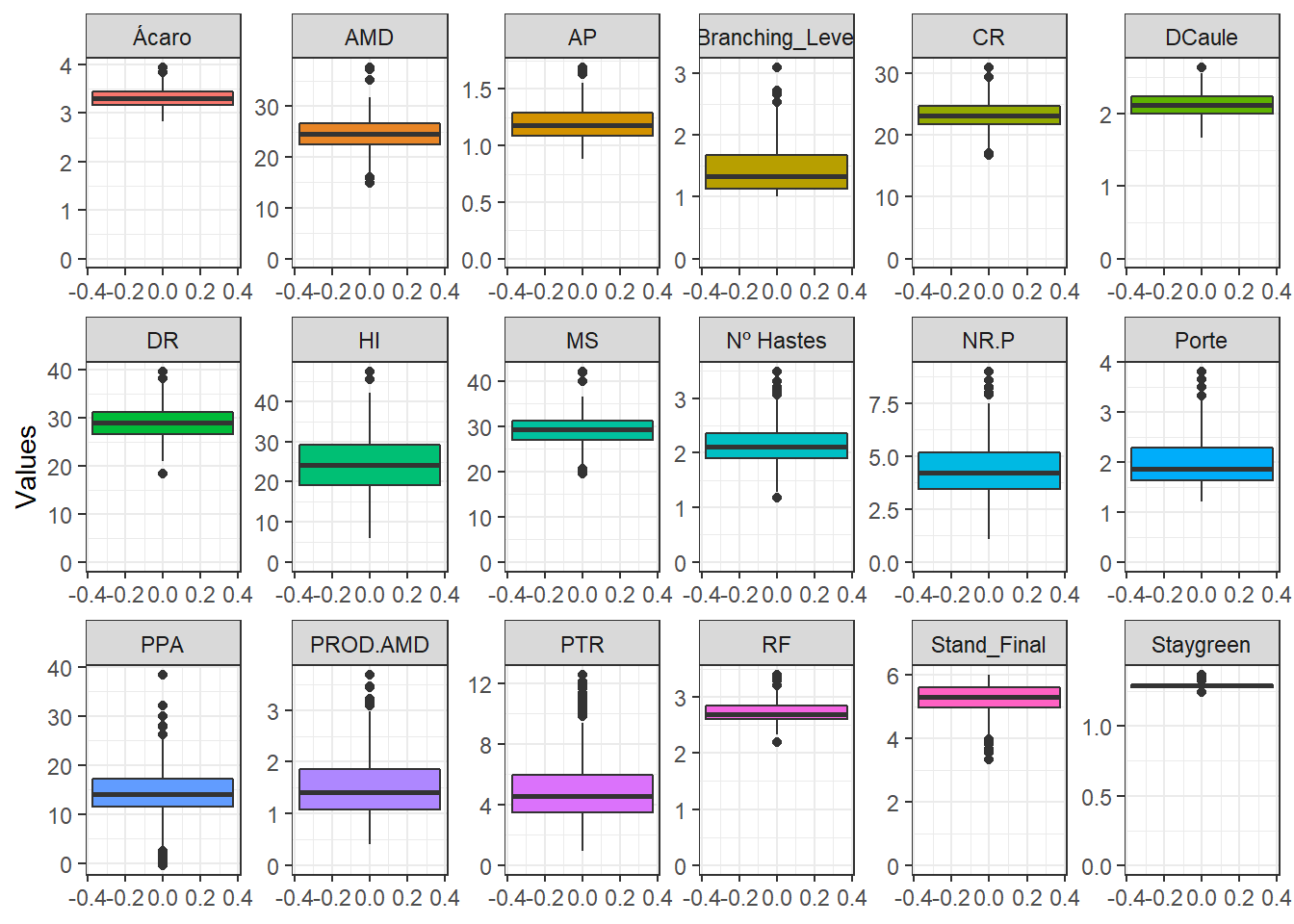

Aqui vamos avaliar apenas a distribuição dos BLUPs sem a média.

BLUPS %>%
  pivot_longer(2:19, names_to = "Variable", values_to = "Values") %>%
  ggplot() +
  geom_density(aes(x = Values), show.legend = FALSE) +
  facet_wrap(. ~ Variable, ncol = 6, scales = "free") +
  expand_limits(y = 0) +
  theme_bw()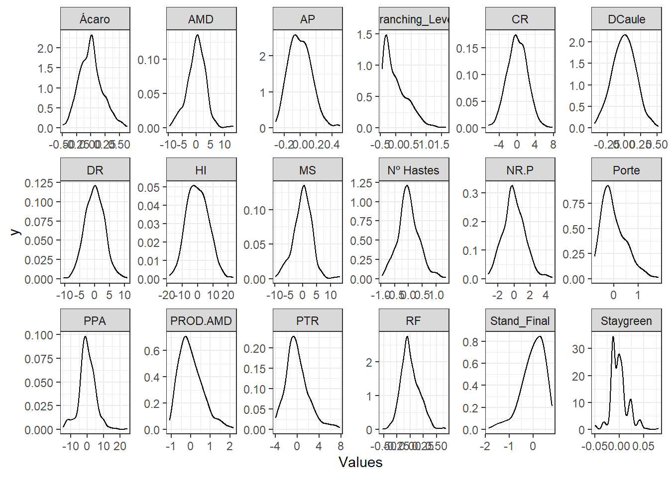

Aparentemente a maioria dos BLUPs para as variáveis seguem distribuição normal e pode ser aplicada a GWS pelos métodos convencionais.

sessionInfo()

R version 4.1.3 (2022-03-10)
Platform: x86_64-w64-mingw32/x64 (64-bit)
Running under: Windows 10 x64 (build 19042)

Matrix products: default

locale:
[1] LC_COLLATE=Portuguese_Brazil.1252  LC_CTYPE=Portuguese_Brazil.1252   
[3] LC_MONETARY=Portuguese_Brazil.1252 LC_NUMERIC=C                      
[5] LC_TIME=Portuguese_Brazil.1252    

attached base packages:
[1] parallel  grid      stats     graphics  grDevices utils     datasets 
[8] methods   base     

other attached packages:
 [1] doParallel_1.0.17     iterators_1.0.14      foreach_1.5.2        
 [4] DataExplorer_0.8.2    metan_1.17.0          readxl_1.4.1         
 [7] data.table_1.14.2     ComplexHeatmap_2.10.0 forcats_0.5.2        
[10] stringr_1.4.1         dplyr_1.0.10          purrr_0.3.4          
[13] readr_2.1.2           tidyr_1.2.1           tibble_3.1.8         
[16] ggplot2_3.3.6         tidyverse_1.3.2       kableExtra_1.3.4     

loaded via a namespace (and not attached):
  [1] minqa_1.2.4         googledrive_2.0.0   colorspace_2.0-3   
  [4] rjson_0.2.21        ellipsis_0.3.2      rprojroot_2.0.3    
  [7] circlize_0.4.15     GlobalOptions_0.1.2 fs_1.5.2           
 [10] clue_0.3-61         rstudioapi_0.14     farver_2.1.1       
 [13] ggrepel_0.9.1       fansi_1.0.3         lubridate_1.8.0    
 [16] mathjaxr_1.6-0      xml2_1.3.3          codetools_0.2-18   
 [19] splines_4.1.3       cachem_1.0.6        knitr_1.40         
 [22] polyclip_1.10-0     jsonlite_1.8.0      nloptr_2.0.3       
 [25] workflowr_1.7.0     broom_1.0.1         cluster_2.1.2      
 [28] dbplyr_2.2.1        png_0.1-7           ggforce_0.4.1      
 [31] compiler_4.1.3      httr_1.4.4          backports_1.4.1    
 [34] Matrix_1.5-1        assertthat_0.2.1    fastmap_1.1.0      
 [37] gargle_1.2.1        cli_3.3.0           later_1.3.0        
 [40] tweenr_2.0.2        htmltools_0.5.3     tools_4.1.3        
 [43] igraph_1.3.5        lmerTest_3.1-3      gtable_0.3.1       
 [46] glue_1.6.2          Rcpp_1.0.9          cellranger_1.1.0   
 [49] jquerylib_0.1.4     vctrs_0.4.1         nlme_3.1-159       
 [52] svglite_2.1.0       xfun_0.32           networkD3_0.4      
 [55] lme4_1.1-30         rvest_1.0.3         lifecycle_1.0.3    
 [58] googlesheets4_1.0.1 MASS_7.3-58.1       scales_1.2.1       
 [61] hms_1.1.2           promises_1.2.0.1    RColorBrewer_1.1-3 
 [64] yaml_2.3.5          gridExtra_2.3       sass_0.4.2         
 [67] reshape_0.8.9       stringi_1.7.6       highr_0.9          
 [70] S4Vectors_0.32.4    BiocGenerics_0.40.0 boot_1.3-28        
 [73] shape_1.4.6         rlang_1.0.6         pkgconfig_2.0.3    
 [76] systemfonts_1.0.4   matrixStats_0.62.0  evaluate_0.17      
 [79] lattice_0.20-45     labeling_0.4.2      htmlwidgets_1.5.4  
 [82] patchwork_1.1.2     tidyselect_1.2.0    GGally_2.1.2       
 [85] plyr_1.8.7          magrittr_2.0.3      R6_2.5.1           
 [88] magick_2.7.3        IRanges_2.28.0      generics_0.1.3     
 [91] DBI_1.1.3           pillar_1.8.1        haven_2.5.1        
 [94] withr_2.5.0         modelr_0.1.9        crayon_1.5.2       
 [97] utf8_1.2.2          tzdb_0.3.0          rmarkdown_2.17     
[100] GetoptLong_1.0.5    git2r_0.30.1        reprex_2.0.2       
[103] digest_0.6.29       webshot_0.5.4       numDeriv_2016.8-1.1
[106] httpuv_1.6.5        stats4_4.1.3        munsell_0.5.0      
[109] viridisLite_0.4.1   bslib_0.4.0

Weverton Gomes da Costa, Pós-Doutorando, Embrapa Mandioca e Fruticultura, wevertonufv@gmail.com ↩︎