Last updated: 2023-06-10
Checks: 6 1
Knit directory: GitHub-with-RStudio-LICAE/
This reproducible R Markdown analysis was created with workflowr (version 1.7.0). The Checks tab describes the reproducibility checks that were applied when the results were created. The Past versions tab lists the development history.
The R Markdown file has unstaged changes. To know which version of
the R Markdown file created these results, you’ll want to first commit
it to the Git repo. If you’re still working on the analysis, you can
ignore this warning. When you’re finished, you can run
wflow_publish to commit the R Markdown file and build the
HTML.
Great job! The global environment was empty. Objects defined in the global environment can affect the analysis in your R Markdown file in unknown ways. For reproduciblity it’s best to always run the code in an empty environment.
The command set.seed(20220715) was run prior to running
the code in the R Markdown file. Setting a seed ensures that any results
that rely on randomness, e.g. subsampling or permutations, are
reproducible.
Great job! Recording the operating system, R version, and package versions is critical for reproducibility.
Nice! There were no cached chunks for this analysis, so you can be confident that you successfully produced the results during this run.
Great job! Using relative paths to the files within your workflowr project makes it easier to run your code on other machines.
Great! You are using Git for version control. Tracking code development and connecting the code version to the results is critical for reproducibility.
The results in this page were generated with repository version 1a7bfd8. See the Past versions tab to see a history of the changes made to the R Markdown and HTML files.
Note that you need to be careful to ensure that all relevant files for
the analysis have been committed to Git prior to generating the results
(you can use wflow_publish or
wflow_git_commit). workflowr only checks the R Markdown
file, but you know if there are other scripts or data files that it
depends on. Below is the status of the Git repository when the results
were generated:
Ignored files:
    Ignored:    .Rproj.user/

Unstaged changes:
    Modified:   analysis/PCA.Rmd
Note that any generated files, e.g. HTML, png, CSS, etc., are not included in this status report because it is ok for generated content to have uncommitted changes.
These are the previous versions of the repository in which changes were
made to the R Markdown (analysis/PCA.Rmd) and HTML
(docs/PCA.html) files. If you’ve configured a remote Git
repository (see ?wflow_git_remote), click on the hyperlinks
in the table below to view the files as they were in that past version.
| File | Version | Author | Date | Message |
|---|---|---|---|---|
| Rmd | 0aac814 | WevertonGomesCosta | 2022-12-14 | Update site |
| html | 0aac814 | WevertonGomesCosta | 2022-12-14 | Update site |
| Rmd | 06cdd23 | WevertonGomesCosta | 2022-08-12 | Update |
| html | 2c52bea | WevertonGomesCosta | 2022-08-12 | Update |
| Rmd | 512947f | WevertonGomesCosta | 2022-08-12 | Update |
| html | 512947f | WevertonGomesCosta | 2022-08-12 | Update |
| html | 6472b7a | WevertonGomesCosta | 2022-08-05 | Update |
| html | f9a57b0 | WevertonGomesCosta | 2022-08-05 | Build site. |
| Rmd | cd7dbb6 | WevertonGomesCosta | 2022-08-05 | wflow_publish(files = "*") |
| html | cd7dbb6 | WevertonGomesCosta | 2022-08-05 | wflow_publish(files = "*") |
Principal Components analysis with Iris data
Collecting data
data <- irisPreparing data for the principal components analysis (PCA)
let’s prepare this prepare this data to plot some boxplot of all the
four traits, for that you will need the function melt of
the reshape2 package and the tidyverse package.
install.packages("reshape2", repos = "https://cloud.r-project.org")Installing package into 'C:/Users/USUARIO/Documents/R/win-library/4.1'
(as 'lib' is unspecified)package 'reshape2' successfully unpacked and MD5 sums checkedWarning: cannot remove prior installation of package 'reshape2'Warning in file.copy(savedcopy, lib, recursive = TRUE): problem copying
C:\Users\USUARIO\Documents\R\win-library\4.1\00LOCK\reshape2\libs\x64\reshape2.dll
to C:\Users\USUARIO\Documents\R\win-library\4.1\reshape2\libs\x64\reshape2.dll:
Permission deniedWarning: restored 'reshape2'
The downloaded binary packages are in
C:\Users\USUARIO\AppData\Local\Temp\RtmpKsJN06\downloaded_packageslibrary(reshape2); library(tidyverse)-- Attaching core tidyverse packages ------------------------ tidyverse 2.0.0 --
v dplyr 1.1.2 v readr 2.1.4
v forcats 1.0.0 v stringr 1.5.0
v ggplot2 3.4.2 v tibble 3.2.1
v lubridate 1.9.2 v tidyr 1.3.0
v purrr 1.0.1 -- Conflicts ------------------------------------------ tidyverse_conflicts() --
x dplyr::filter() masks stats::filter()
x dplyr::lag() masks stats::lag()
i Use the conflicted package (<http://conflicted.r-lib.org/>) to force all conflicts to become errorsdataMelted <- data %>% reshape2::melt(data = .,
id.vars = "Species",
variable.name = "trait",
value.name = "y")
head(dataMelted) Species trait y
1 setosa Sepal.Length 5.1
2 setosa Sepal.Length 4.9
3 setosa Sepal.Length 4.7
4 setosa Sepal.Length 4.6
5 setosa Sepal.Length 5.0
6 setosa Sepal.Length 5.4Great, now we have the data at the format to make boxplot from all
traits at the same code line. so lets keep moving. For that we will use
ggplot2 package.
dataMelted %>% ggplot(aes(x = Species, y = y, fill = Species)) +
     geom_boxplot() + facet_wrap(~trait, scales = "free_y") +
     theme(legend.position = "none")
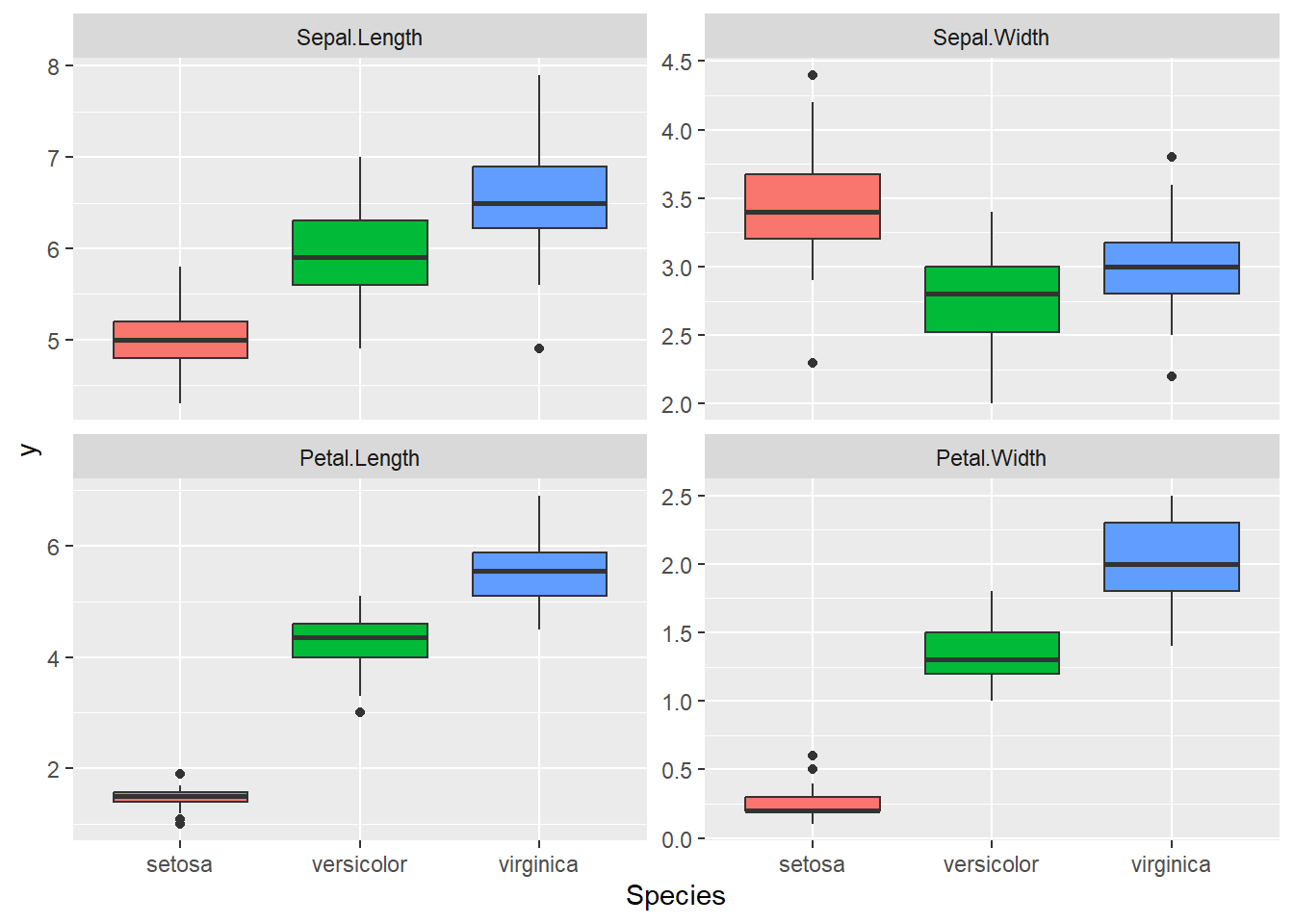
Great data, we can see a lot of differences between the
Species for these traits. It seems that we may have some
correlation between Petal Length and Width. We
also have different amplitude for these traits this will certainly
results in different phenotypic variance between the
traits, so we need to scale these traits before the
PCA.
DataSc <- data %>% select(-Species) %>%
     scale(x = ., center = TRUE, scale = TRUE) %>%
     as.data.frame() %>%
     mutate(Species = data$Species)
head(DataSc)
Sepal.Length Sepal.Width Petal.Length Petal.Width Species
1 -0.8976739 1.01560199 -1.335752 -1.311052 setosa
2 -1.1392005 -0.13153881 -1.335752 -1.311052 setosa
3 -1.3807271 0.32731751 -1.392399 -1.311052 setosa
4 -1.5014904 0.09788935 -1.279104 -1.311052 setosa
5 -1.0184372 1.24503015 -1.335752 -1.311052 setosa
6 -0.5353840 1.93331463 -1.165809 -1.048667 setosaPrincipal Component Analysis (PCA)
So let’s proceed for the PCA analysis, here we will use the
prcomp function from R status package, so no
need to call any package.
PCA <- prcomp(DataSc %>% select(-Species))Saving results
Let’s save the important results in objects, so we could make some
graphs with them.
1. Accumulate percent of the total phenotypic variance explained by the principal components (PC)
Perc <- 100 * PCA$sdev^2 / sum(PCA$sdev^2)

PercAc <- as.vector(rep(NA, times = length(Perc)))
for(i in 1:length(Perc)) {
  PercAc[i] <- sum(Perc[1:i])
  names(PercAc)[i] <- i
}
names(PercAc) <- c("PC1", "PC2", "PC3", "PC4")
PercAc
PC1 PC2 PC3 PC4
72.96245 95.81321 99.48213 100.00000 Oh these data are high correlated.
2. Correlations of the traits with the principal components (PC)
CorTraits <- PCA$rotation
rownames(CorTraits) <- c("SepLen", "SepWid", "PetLen", "PetWid")
CorTraits
PC1 PC2 PC3 PC4
SepLen 0.5210659 -0.37741762 0.7195664 0.2612863
SepWid -0.2693474 -0.92329566 -0.2443818 -0.1235096
PetLen 0.5804131 -0.02449161 -0.1421264 -0.8014492
PetWid 0.5648565 -0.06694199 -0.6342727 0.5235971LabelsPCA <- CorTraits %>% as.data.frame %>%
mutate(PC1 = PC1 + 0.15, .keep = "unused")3. Individuals scores for the principal components (PC)
ScoresSpecies <- PCA$x %>%
     as.data.frame %>%
     mutate(Species = data$Species)

head(ScoresSpecies)
PC1 PC2 PC3 PC4 Species
1 -2.257141 -0.4784238 0.12727962 0.024087508 setosa
2 -2.074013 0.6718827 0.23382552 0.102662845 setosa
3 -2.356335 0.3407664 -0.04405390 0.028282305 setosa
4 -2.291707 0.5953999 -0.09098530 -0.065735340 setosa
5 -2.381863 -0.6446757 -0.01568565 -0.035802870 setosa
6 -2.068701 -1.4842053 -0.02687825 0.006586116 setosaGreat we got what we need to create our figures.
Figures
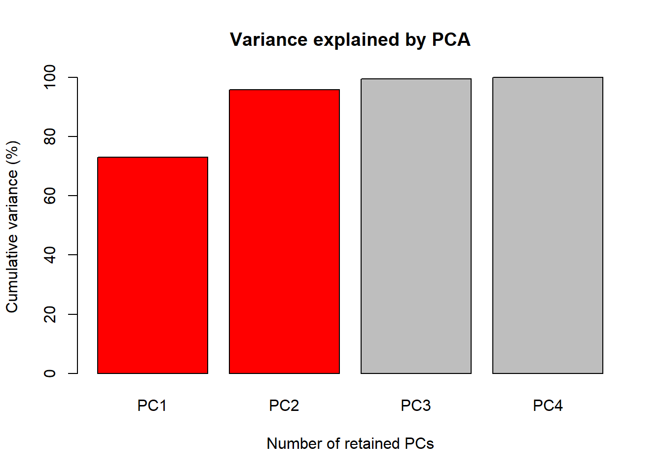
The first figure will be a barplot of the accumulated variances
explained by the PC. We will use the color red the PC
selected to use at the next figures.
barplot(PercAc, main = "Variance explained by PCA",
        ylab = "Cumulative variance (%)", xlab = "Number of retained PCs",
        col = c("red", "red", "gray", "gray", "gray"))
R markdown allows us to hide the code that create the figure, this
could be done adding the argument echo = FALSE inside the
curly brackets at the chunk. Using echo argument will print
just the result of you chunk, link below.

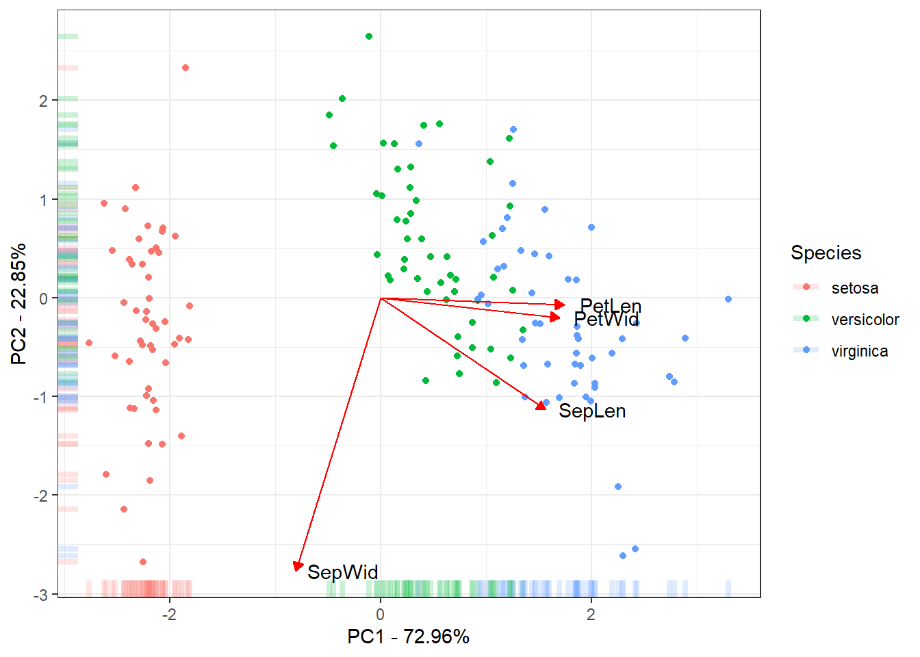
The last figure will be a scatter plot of the individuals with their score for the first two PCs with the correlation of the traits with the first two PCs.
ggplot(data = ScoresSpecies, aes(x = PC1, y = PC2, color = Species)) +
  geom_point() + geom_rug(alpha = 0.2, size = 1.5) +
  geom_segment(mapping = aes(x = 0, xend = 3*PC1, y = 0, yend = 3*PC2),
               colour = "red",
               data = CorTraits %>% as.data.frame,
               arrow = arrow(type = "closed",
                             length = unit(0.2,units = "cm"))) +
  geom_text(mapping = aes(x = PC1*3, y = PC2*3, label = rownames(LabelsPCA)),
            data = LabelsPCA, colour = "black") +
  theme_bw() +
  xlab(paste("PC1 - ", round(Perc[1], digits = 2), "%", sep = "")) +
     ylab(paste("PC2 - ", round(Perc[2], digits = 2), "%", sep = ""))
Warning: Using `size` aesthetic for lines was deprecated in ggplot2 3.4.0.
i Please use `linewidth` instead.
This warning is displayed once every 8 hours.
Call `lifecycle::last_lifecycle_warnings()` to see where this warning was
generated.
This is the final results of the PC. Mostly of the variance explained
by the 1˚PC is due to the between species Setosa Vs
Versicolor and Virginica. The 2˚PC just
explain variance within the species. Also the traits
Petal Length, Petal Width and
Sepal Length could be used to discriminate the species.
sessionInfo()R version 4.1.3 (2022-03-10)
Platform: x86_64-w64-mingw32/x64 (64-bit)
Running under: Windows 10 x64 (build 19045)
Matrix products: default
locale:
[1] LC_COLLATE=Portuguese_Brazil.1252 LC_CTYPE=Portuguese_Brazil.1252
[3] LC_MONETARY=Portuguese_Brazil.1252 LC_NUMERIC=C
[5] LC_TIME=Portuguese_Brazil.1252
attached base packages:
[1] stats graphics grDevices utils datasets methods base
other attached packages:
[1] lubridate_1.9.2 forcats_1.0.0 stringr_1.5.0 dplyr_1.1.2
[5] purrr_1.0.1 readr_2.1.4 tidyr_1.3.0 tibble_3.2.1
[9] ggplot2_3.4.2 tidyverse_2.0.0 reshape2_1.4.4
loaded via a namespace (and not attached):
[1] tidyselect_1.2.0 xfun_0.38 bslib_0.4.2 colorspace_2.1-0
[5] vctrs_0.6.1 generics_0.1.3 htmltools_0.5.5 yaml_2.3.7
[9] utf8_1.2.3 rlang_1.1.0 jquerylib_0.1.4 later_1.3.0
[13] pillar_1.9.0 glue_1.6.2 withr_2.5.0 lifecycle_1.0.3
[17] plyr_1.8.8 munsell_0.5.0 gtable_0.3.3 workflowr_1.7.0
[21] evaluate_0.20 labeling_0.4.2 knitr_1.42 tzdb_0.3.0
[25] fastmap_1.1.1 httpuv_1.6.9 fansi_1.0.4 highr_0.10
[29] Rcpp_1.0.10 promises_1.2.0.1 scales_1.2.1 cachem_1.0.7
[33] jsonlite_1.8.4 farver_2.1.1 fs_1.6.1 hms_1.1.3
[37] digest_0.6.31 stringi_1.7.12 rprojroot_2.0.3 grid_4.1.3
[41] cli_3.6.1 tools_4.1.3 magrittr_2.0.3 sass_0.4.5
[45] crayon_1.5.2 whisker_0.4.1 pkgconfig_2.0.3 timechange_0.2.0
[49] rmarkdown_2.21 rstudioapi_0.14 R6_2.5.1 git2r_0.30.1
[53] compiler_4.1.3 Weverton Gomes da Costa, Pós-Doutorando, Departamento de Estatística - UFV, wevertonufv@gmail.com↩︎