ld decay
Costa, W. G.
2025-03-26
Last updated: 2025-03-26
Checks: 6 1
Knit directory:
Importance-of-markers-for-QTL-detection-by-machine-learning-methods/
This reproducible R Markdown analysis was created with workflowr (version 1.7.1). The Checks tab describes the reproducibility checks that were applied when the results were created. The Past versions tab lists the development history.
The R Markdown file has unstaged changes. To know which version of
the R Markdown file created these results, you’ll want to first commit
it to the Git repo. If you’re still working on the analysis, you can
ignore this warning. When you’re finished, you can run
wflow_publish to commit the R Markdown file and build the
HTML.
Great job! The global environment was empty. Objects defined in the global environment can affect the analysis in your R Markdown file in unknown ways. For reproduciblity it’s best to always run the code in an empty environment.
The command set.seed(20221222) was run prior to running
the code in the R Markdown file. Setting a seed ensures that any results
that rely on randomness, e.g. subsampling or permutations, are
reproducible.
Great job! Recording the operating system, R version, and package versions is critical for reproducibility.
Nice! There were no cached chunks for this analysis, so you can be confident that you successfully produced the results during this run.
Great job! Using relative paths to the files within your workflowr project makes it easier to run your code on other machines.
Great! You are using Git for version control. Tracking code development and connecting the code version to the results is critical for reproducibility.
The results in this page were generated with repository version afa31ca. See the Past versions tab to see a history of the changes made to the R Markdown and HTML files.
Note that you need to be careful to ensure that all relevant files for
the analysis have been committed to Git prior to generating the results
(you can use wflow_publish or
wflow_git_commit). workflowr only checks the R Markdown
file, but you know if there are other scripts or data files that it
depends on. Below is the status of the Git repository when the results
were generated:
Ignored files:
    Ignored:    .Rproj.user/

Unstaged changes:
    Modified:   analysis/ld_decay.Rmd
Note that any generated files, e.g. HTML, png, CSS, etc., are not included in this status report because it is ok for generated content to have uncommitted changes.
These are the previous versions of the repository in which changes were
made to the R Markdown (analysis/ld_decay.Rmd) and HTML
(docs/ld_decay.html) files. If you’ve configured a remote
Git repository (see ?wflow_git_remote), click on the
hyperlinks in the table below to view the files as they were in that
past version.
| File | Version | Author | Date | Message |
|---|---|---|---|---|
| Rmd | 06c2d7d | WevertonGomesCosta | 2025-03-25 | update ld_decay.Rmd with plot |
| Rmd | d57532f | WevertonGomesCosta | 2025-03-25 | add ld_decay.rmd |
Load necessary libraries
Carregando pacotes exigidos: MatrixCarregando pacotes exigidos: MASSCarregando pacotes exigidos: crayon
Anexando pacote: 'ggplot2'O seguinte objeto é mascarado por 'package:crayon':
%+%
Anexando pacote: 'dplyr'O seguinte objeto é mascarado por 'package:MASS':
selectOs seguintes objetos são mascarados por 'package:stats':
filter, lagOs seguintes objetos são mascarados por 'package:base':
intersect, setdiff, setequal, unionLoad genotype data
  V1 V2 V3 V4 V5
1  0  0  0  0  0
2  0  0  0  0  0
3  0  0  0  0  0
4 -1 -1 -1 -1 -1
5  0  0  0  0  0
6  0  0  0  0  0
Load and prepare map data
mapCP <- readRDS("data/map.rds") %>%
  mutate(
    Locus = paste0("V", 1:n()),
    Position = as.numeric(Tamanho),
    LG = as.integer(GL)
  ) %>%
  dplyr::select(Locus, Position, LG)

str(mapCP)
'data.frame': 4010 obs. of 3 variables:
$ Locus : chr "V1" "V2" "V3" "V4" ...
$ Position: num 0 0.5 1 1.5 2 2.5 3 3.5 4 4.5 ...
$ LG : int 1 1 1 1 1 1 1 1 1 1 ... Locus Position LG
Length:4010 Min. : 0 Min. : 1.0
Class :character 1st Qu.: 50 1st Qu.: 3.0
Mode :character Median :100 Median : 5.5
Mean :100 Mean : 5.5
3rd Qu.:150 3rd Qu.: 8.0
Max. :200 Max. :10.0 Run LD decay analysis for each linkage group
Step 1: Obtain a sorted list of unique linkage groups from the map data
Step 2: Apply a function to each linkage group using lapply
res <- lapply(unique_LGs, function(lg) {
  # Step 2a: For the current linkage group 'lg', extract the corresponding marker names
  markers <- mapCP %>%
    filter(LG == lg) %>%  # Filter the map data to include only rows where LG equals the current linkage group
    pull(Locus)           # Extract the 'Locus' column, which contains marker names

  # Step 2b: Perform Linkage Disequilibrium (LD) decay analysis on the genotype data for these markers
  LDDecay <- LD.decay(CPgeno[, markers], # Subset the genotype matrix to include only the columns for the current markers
                      mapCP %>% filter(LG == lg))  # Subset the map data to include only the current linkage group

  # Step 2c: Filter the LD results to include only significant marker pairs after Bonferroni correction
  A <- LDDecay$all.LG %>%  # Access the LD results for all marker pairs
    filter(p < 0.05 / choose(length(markers), 2))  # Apply Bonferroni correction to adjust the p-value threshold

  # Step 2d: Check if there are any significant marker pairs
  if (nrow(A) > 0) {
    # If significant pairs exist, create a data frame including the linkage group identifier
    data.frame(GL = paste0("lg", lg), # Add a column 'GL' with the linkage group name (e.g., 'lg1', 'lg2', etc.)
               A)                       # Include the filtered LD decay results
  } else {
    # If no significant pairs are found, return NULL for this linkage group
    NULL
  }
})
| | | 0% | |======================================================================| 100% | | | 0% | |======================================================================| 100% | | | 0% | |======================================================================| 100% | | | 0% | |======================================================================| 100% | | | 0% | |======================================================================| 100% | | | 0% | |======================================================================| 100% | | | 0% | |======================================================================| 100% | | | 0% | |======================================================================| 100% | | | 0% | |======================================================================| 100% | | | 0% | |======================================================================| 100%Combine results and remove NULLs
Predict r² values for a sequence of distances
Find the distance where r² is approximately 0.2
target_r2 <- 0.87
closest_index <- which.min(abs(pred - target_r2))
closest_d <- d_seq[closest_index]
closest_d
[1] 2.6Plot the LD decay curve
library(ggrepel)

# Create the plot with additional adjustments
color_palette <- colorRampPalette(c('black', 'gray50'))
p <- ggplot(dados, aes(x = d, y = r2, colour = GL)) +
  geom_point(pch = 21, show.legend = FALSE) +
  geom_line(
    data = data_pred,
    aes(x = d, y = pred),
    colour = 'red',
    linewidth = 1
  ) +
  geom_hline(yintercept = target_r2,
             linetype = "dashed",
             color = "blue") +
  geom_vline(xintercept = closest_d,
             linetype = "dashed",
             color = "green") +
  geom_point(
    aes(x = closest_d, y = target_r2),
    data = NULL,
    color = "gold",
    size = 3
  ) +
  scale_color_manual(values = color_palette(length(unique(dados$GL)))) +
  scale_y_continuous(breaks = seq(0, 1, by = 0.1)) +
  scale_x_continuous(breaks = seq(0, max(dados$d), by = 10)) +
  labs(x = "Distance (d)", y = expression(r^2)) +
  theme_classic() +
  theme(text = element_text(size = 20))

p +
  geom_text(
    aes(
      x = closest_d + 15,
      y = target_r2,
      label = paste("d =", round(closest_d, 2), "cM")
    ),
    data = NULL,
    nudge_y = 0.02,
    color = "black",
    fontface = "bold"
  )
Warning in geom_point(aes(x = closest_d, y = target_r2), data = NULL, color = "gold", : All aesthetics have length 1, but the data has 806010 rows.
ℹ Please consider using `annotate()` or provide this layer with data containing
a single row.Warning in geom_text(aes(x = closest_d + 15, y = target_r2, label = paste("d =", : All aesthetics have length 1, but the data has 806010 rows.
ℹ Please consider using `annotate()` or provide this layer with data containing
a single row.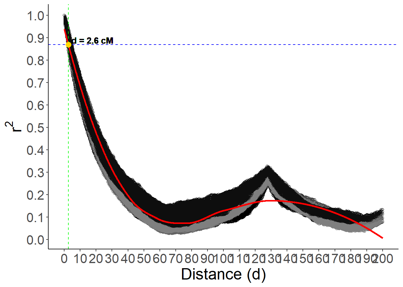
R version 4.4.3 (2025-02-28 ucrt)
Platform: x86_64-w64-mingw32/x64
Running under: Windows 11 x64 (build 26100)

Matrix products: default


locale:
[1] LC_COLLATE=Portuguese_Brazil.utf8  LC_CTYPE=Portuguese_Brazil.utf8
[3] LC_MONETARY=Portuguese_Brazil.utf8 LC_NUMERIC=C
[5] LC_TIME=Portuguese_Brazil.utf8

time zone: America/Sao_Paulo
tzcode source: internal

attached base packages:
[1] stats     graphics  grDevices utils     datasets  methods   base

other attached packages:
[1] ggrepel_0.9.6 dplyr_1.1.4   ggplot2_3.5.1 sommer_4.3.7  crayon_1.5.3
[6] MASS_7.3-64   Matrix_1.7-2

loaded via a namespace (and not attached):
 [1] gtable_0.3.6      jsonlite_1.9.1    compiler_4.4.3    promises_1.3.2
 [5] tidyselect_1.2.1  Rcpp_1.0.14       stringr_1.5.1     git2r_0.35.0
 [9] later_1.4.1       jquerylib_0.1.4   scales_1.3.0      yaml_2.3.10
[13] fastmap_1.2.0     lattice_0.22-6    R6_2.6.1          generics_0.1.3
[17] workflowr_1.7.1   knitr_1.49        tibble_3.2.1      munsell_0.5.1
[21] rprojroot_2.0.4   bslib_0.9.0       pillar_1.10.1     rlang_1.1.5
[25] cachem_1.1.0      stringi_1.8.4     httpuv_1.6.15     xfun_0.51
[29] fs_1.6.5          sass_0.4.9        cli_3.6.4         withr_3.0.2
[33] magrittr_2.0.3    digest_0.6.37     grid_4.4.3        rstudioapi_0.17.1
[37] lifecycle_1.0.4   vctrs_0.6.5       evaluate_1.0.3    glue_1.8.0
[41] farver_2.1.2      whisker_0.4.1     colorspace_2.1-1  rmarkdown_2.29
[45] tools_4.4.3       pkgconfig_2.0.3   htmltools_0.5.8.1