Last updated: 2025-10-04

Checks: 6 1

Knit directory: analisys-next-gen-2022/

This reproducible R Markdown analysis was created with workflowr (version 1.7.2). The Checks tab describes the reproducibility checks that were applied when the results were created. The Past versions tab lists the development history.

R Markdown file: uncommitted changes

The R Markdown file has unstaged changes. To know which version of the R Markdown file created these results, you’ll want to first commit it to the Git repo. If you’re still working on the analysis, you can ignore this warning. When you’re finished, you can run wflow_publish to commit the R Markdown file and build the HTML.

Environment: empty

Great job! The global environment was empty. Objects defined in the global environment can affect the analysis in your R Markdown file in unknown ways. For reproduciblity it’s best to always run the code in an empty environment.

Seed: set.seed(20251003)

The command set.seed(20251003) was run prior to running the code in the R Markdown file. Setting a seed ensures that any results that rely on randomness, e.g. subsampling or permutations, are reproducible.

Session information: recorded

Great job! Recording the operating system, R version, and package versions is critical for reproducibility.

Cache: none

Nice! There were no cached chunks for this analysis, so you can be confident that you successfully produced the results during this run.

File paths: relative

Great job! Using relative paths to the files within your workflowr project makes it easier to run your code on other machines.

Repository version: d75043a

Great! You are using Git for version control. Tracking code development and connecting the code version to the results is critical for reproducibility.

The results in this page were generated with repository version d75043a. See the Past versions tab to see a history of the changes made to the R Markdown and HTML files.

Note that you need to be careful to ensure that all relevant files for the analysis have been committed to Git prior to generating the results (you can use wflow_publish or wflow_git_commit). workflowr only checks the R Markdown file, but you know if there are other scripts or data files that it depends on. Below is the status of the Git repository when the results were generated:


Ignored files:
    Ignored:    .Rproj.user/
    Ignored:    data/Arquivos Fieldbook 2022/BR.AYTInd.22.CMa_1.xls
    Ignored:    data/Arquivos Fieldbook 2022/BR.AYTInd.22.Candeal 8MP e 16cm_1.xls
    Ignored:    data/Arquivos Fieldbook 2022/BR.AYTInd.22.Estab_1.xls
    Ignored:    data/Arquivos Fieldbook 2022/BR.AYTInd.22.NH 16CM_1.xls
    Ignored:    data/Arquivos Fieldbook 2022/BR.AYTM.22.Candeal_1.xls
    Ignored:    data/Arquivos Fieldbook 2022/BR.AYTM.22.Estab_1.xls
    Ignored:    data/Arquivos Fieldbook 2022/BR.AYTM.22.NH1_1.xls
    Ignored:    data/Arquivos Fieldbook 2022/BR.AYTM.22.NH_1.xls
    Ignored:    data/Arquivos Fieldbook 2022/BR.AYTM.22.Pureza_1.xls
    Ignored:    data/Arquivos Fieldbook 2022/BR.AYTM.Candeal.22_1.xls
    Ignored:    data/Arquivos Fieldbook 2022/BR.CBGS-C4.22.CNPMF_1.xls
    Ignored:    data/Arquivos Fieldbook 2022/BR.CET.22.CNPMF.xls
    Ignored:    data/Arquivos Fieldbook 2022/BR.MULTGS-C3.22.Podium_1.xls
    Ignored:    data/Arquivos Fieldbook 2022/BR.MultGS.22.NH_1.xls
    Ignored:    data/Arquivos Fieldbook 2022/BR.PTBAG.22.Candeal Florescimento_1.xls
    Ignored:    data/Arquivos Fieldbook 2022/BR.PYT.22.Candeal_1.xls
    Ignored:    data/Arquivos Fieldbook 2022/BR.PYT.22.Jaguaripe_1.xls
    Ignored:    data/Arquivos Fieldbook 2022/BR.PYTO.22.Lon_1.xls
    Ignored:    data/Arquivos Fieldbook 2022/BR.UYT.22.Jagua_1.xls
    Ignored:    data/Arquivos Fieldbook 2022/BR.UYT.22.TRAC_1.xls
    Ignored:    data/Arquivos Fieldbook 2022/BR.UYT.WD.22.BJL_1.xls
    Ignored:    data/Arquivos Fieldbook 2022/BR.UYTGS.22.CMa_1.xls
    Ignored:    data/Arquivos Fieldbook 2022/BR.UYTGS.22.COMG_1.xls
    Ignored:    data/Arquivos Fieldbook 2022/BR.UYTGS.22.Candeal_1.xls
    Ignored:    data/Arquivos Fieldbook 2022/BR.UYTGS.22.CoC_1.xls
    Ignored:    data/Arquivos Fieldbook 2022/BR.UYTGS.22.CoH_1.xls
    Ignored:    data/Arquivos Fieldbook 2022/BR.UYTGS.22.ER_1.xls
    Ignored:    data/Arquivos Fieldbook 2022/BR.UYTGS.22.Esp_1.xls
    Ignored:    data/Arquivos Fieldbook 2022/BR.UYTGS.22.Estab_1.xls
    Ignored:    data/Arquivos Fieldbook 2022/BR.UYTGS.22.IFGua_1.xls
    Ignored:    data/Arquivos Fieldbook 2022/BR.UYTGS.22.ItiBA_1.xls
    Ignored:    data/Arquivos Fieldbook 2022/BR.UYTGS.22.LagDa_1.xls
    Ignored:    data/Arquivos Fieldbook 2022/BR.UYTGS.22.Mara_1.xls
    Ignored:    data/Arquivos Fieldbook 2022/BR.UYTGS.22.Mont_1.xls
    Ignored:    data/Arquivos Fieldbook 2022/BR.UYTGS.22.NH1_1.xls
    Ignored:    data/Arquivos Fieldbook 2022/BR.UYTGS.22.NH_1.xls
    Ignored:    data/Arquivos Fieldbook 2022/BR.UYTGS.22.PAMG_1.xls
    Ignored:    data/Arquivos Fieldbook 2022/BR.UYTGS.22.Quiss_1.xls
    Ignored:    data/Arquivos Fieldbook 2022/BR.UYTGS.22.SA_1.xls
    Ignored:    data/Arquivos Fieldbook 2022/BR.UYTGS.22.SDAP_1.xls
    Ignored:    data/Arquivos Fieldbook 2022/BR.UYTGS.22.TRAC_1.xls
    Ignored:    data/Arquivos Fieldbook 2022/BR.UYTGS.22.VC_1.xls
    Ignored:    data/phenotype.csv
    Ignored:    output/StudyTraits.tiff
    Ignored:    output/StudyYear.tiff

Untracked files:
    Untracked:  output/SUMMARY OF FIELD TRIALS.csv
    Untracked:  output/SUMMARY OF FIELD TRIALS_UYT.csv
    Untracked:  output/accession_number.csv

Unstaged changes:
    Modified:   analysis/1_Trials-and-traits-2023.Rmd

Note that any generated files, e.g. HTML, png, CSS, etc., are not included in this status report because it is ok for generated content to have uncommitted changes.

These are the previous versions of the repository in which changes were made to the R Markdown (analysis/1_Trials-and-traits-2023.Rmd) and HTML (docs/1_Trials-and-traits-2023.html) files. If you’ve configured a remote Git repository (see ?wflow_git_remote), click on the hyperlinks in the table below to view the files as they were in that past version.

File	Version	Author	Date	Message
Rmd	4edf925	WevertonGomesCosta	2025-10-04	add scripts rmd

Ótimo, Weverton 🙌. O código já está bem estruturado, mas podemos refinar as descrições, comentários e interpretações para deixá-lo mais didático e profissional, no estilo de um tutorial científico. Veja a versão aprimorada:

Introduction

This script analyzes the number of cassava field trials and traits evaluated per year in the Embrapa Cassava Breeding Program, using data from CassavaBase.
The objective is to quantify the expansion of the breeding program in terms of experimental trials and phenotypic traits, and to provide a detailed summary of the trials conducted in 2022/2023.

We will go through the following steps:

Load required packages
Import metadata from CassavaBase
Calculate and plot the number of trials per year
Calculate and plot the number of traits per year
Generate summary tables of traits evaluated
Summarize the number of trials and clones in 2022/2023

Step 1: Loading Packages

We start by loading the main R packages used in the analysis.
Each package plays a specific role:
- ggthemes / grafify → improve the aesthetics of plots
- tidyverse → data wrangling and visualization
- readxl → import Excel spreadsheets
- data.table → efficient handling of large datasets
- genomicMateSelectR → integration with CassavaBase data formats
- janitor → cleaning and reshaping data tables

library(ggthemes)          # Themes for ggplot2
library(grafify)           # Color palettes for plots
library(tidyverse)         # Data manipulation and visualization
library(readxl)            # Import Excel files
library(data.table)        # Efficient data handling
library(genomicMateSelectR)# CassavaBase data integration
library(janitor)           # Data cleaning helpers

Step 2: Importing Metadata

We import the metadata file (metadata1.csv), which contains information about each trial (year, location, design, etc.).
This dataset is the foundation for calculating the number of trials per year.

dbdata <- read_delim(
  "data/metadata1.csv",
  delim = ";",
  escape_double = FALSE,
  trim_ws = TRUE
)

Step 3: Number of Trials per Year

Here we calculate the number of trials conducted each year.
- We exclude 2023, since data collection was incomplete at the time of analysis.
- We reformat the year as a crop cycle (e.g., 2021/2022).
- We group by year and count the number of trials.
- For 2022/2023, we manually adjust the count to 49 trials (based on fieldbook records).

number_trials_year <- dbdata %>%
  filter(studyYear != "2023") %>% 
  droplevels() %>% 
  mutate(
    studyYear = paste0(studyYear, "/", studyYear + 1),
    studyYear = as.factor(studyYear)
  ) %>%
  group_by(studyYear) %>%
  tally() %>% 
  mutate(n = ifelse(studyYear == "2022/2023", 49, n))

write.table(number_trials_year, "output/number_trials_year.csv", sep = ",", row.names = F)

Plotting the number of trials

We visualize the number of trials per year using a bar chart.
Labels above the bars indicate the exact number of trials, and the subtitle shows the total across all years.

number_trials_year %>%
  ggplot() +
  geom_col(aes(x = studyYear, y = n, fill = studyYear), show.legend = F) +
  geom_text(aes(x = studyYear, y = n + 1, label = n), size = 2, vjust = 0) +
  theme_bw() +
  scale_fill_grafify(palette = "kelly") +
  labs(
    title = "Number of trials inserted in CassavaBase - EMBRAPA",
    subtitle = paste("Total number of trials = ", sum(number_trials_year$n)),
    x = "Study Year",
    y = "Number of Trials Inserted"
  ) +
  theme(text = element_text(size = 10),
        axis.text.x = element_text(face ="bold", angle = 45, hjust = 1))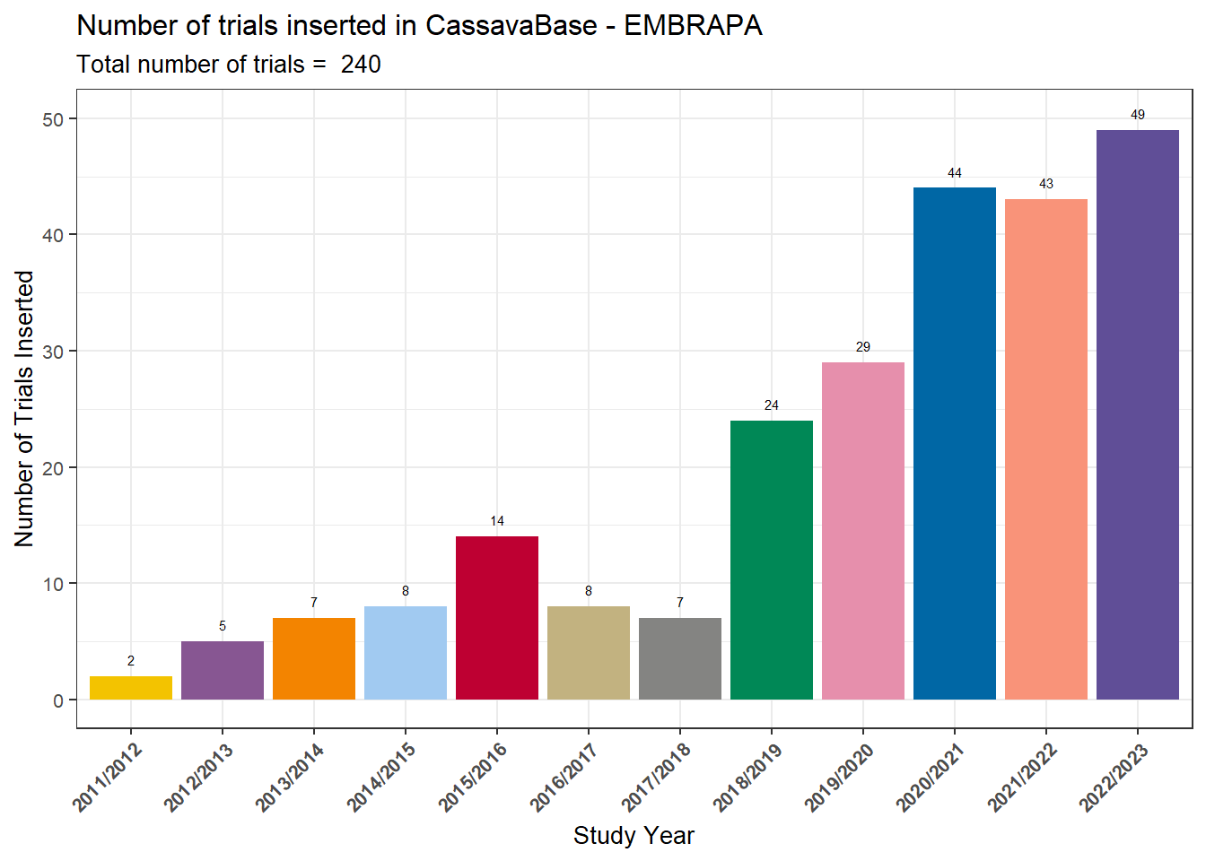

ggsave("output/StudyYear.tiff", width = 16, height = 8)

Interpretation:
The plot shows a steady increase in the number of trials since 2018, reflecting the program’s expansion and the systematic effort to document experiments in CassavaBase.

Step 4: Number of Traits per Year

Next, we calculate how many traits were evaluated each year.
- We select only trait columns from the phenotype dataset.
- For each year, we compute whether a trait was measured (1) or not (0).
- We then sum across traits to obtain the total number of traits evaluated per year.

dbdata <- readDBdata(phenotypeFile = here::here("data", "phenotype.csv"))

number_traits_year <- dbdata %>%
  select(studyYear,
         amylose.content.in.ug.g.percentage.CO_334.0000075:total.carotenoid.by.iCheck.method.CO_334.0000162) %>%
  group_by(studyYear) %>%
  summarise(across(
    everything(),
    ~ if (is.numeric(.)) mean(., na.rm = TRUE) else first(.)
  )) %>%
  mutate(studyYear = paste0(studyYear, "/", studyYear + 1),
         studyYear = as.factor(studyYear)) %>%
  mutate(across(where(is.numeric), ~ ifelse(is.na(.), 0, 1))) %>%
  mutate(sum = rowSums(select(., where(is.numeric)), na.rm = TRUE))

Plotting the number of traits

number_traits_year %>%
  select(where(~ n_distinct(.) > 1)) %>%
  ggplot() +
  geom_col(aes(x = studyYear, y = sum, fill = studyYear), show.legend = F) +
  geom_text(aes(x = studyYear, y = sum, label = sum), vjust = -0.5, size = 2) +
  theme_bw() +
  scale_fill_brewer(palette = "Paired") +
  labs(
    title = "Number of traits evaluated by year in CassavaBase - EMBRAPA",
    subtitle = paste("Total number of traits = ", ncol(number_traits_year) - 1),
    x = "Study Year",
    y = "Number of traits evaluated"
  ) +
  theme(text = element_text(size = 10),
        axis.text.x = element_text(face ="bold", angle = 45, hjust = 1))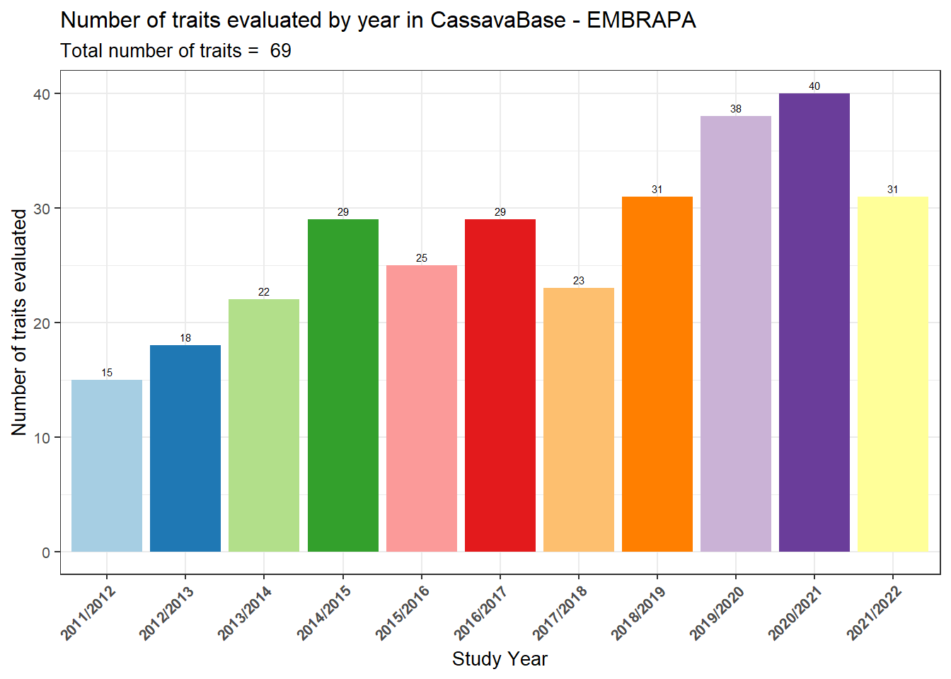

ggsave("output/StudyTraits.tiff", width = 16, height = 8)

Interpretation:
The number of traits evaluated has increased over time, reaching 69 traits in total.
This demonstrates the program’s effort to integrate yield, quality, and stress tolerance traits into the breeding pipeline, moving beyond simple yield evaluation.

Step 5: Trait Table

Finally, we generate a trait-by-year table.
This table indicates with an “x” whether a given trait was evaluated in a specific year, providing a quick overview of trait coverage across years.

number_traits_year2 <- number_traits_year %>%
  select(-sum) %>%
  t() %>%
  row_to_names(row_number = 1) %>%
  as_tibble(rownames = "Trait") %>%
  mutate(across(c(2:12), ~ ifelse(. == 1, "x", NA)))

write.table(number_traits_year2, "output/number_traits_year2.csv", sep = ",", row.names = F)

Interpretation:
This table is useful for identifying when each trait started being measured and for tracking the evolution of phenotyping priorities in the breeding program.

Step 6: Trials and Clones in 2022/2023

Now we focus on the field trials conducted in 2022/2023.
This step summarizes the number of trials and the number of clones evaluated in each trial type (AYT, PYT, UYT, MULT, CB).

trials_22 <- list.files(path = "data/Arquivos Fieldbook 2022",
                        pattern = "BR.",
                        full.names = T) %>%
  set_names() %>%
  map_df(~ read_excel(., .name_repair = janitor::make_clean_names), .id = "sheet") %>%
  mutate(
    trial_type = toupper(str_split_i(plot_name, '[.]', 2)),
    trial = paste("BR", trial_type, "22", sep = "."),
    locate = ifelse(sheet == "data/Arquivos Fieldbook 2022/BR.UYT.WD.22.BJL_1.xls",
                    str_split_i(plot_name, '[.]', 3),
                    str_split_i(plot_name, '[.]', -2))
  )

Step 6.1: Number of Accessions (Clones)

We calculate the number of unique clones evaluated per trial type.

accession_number <- trials_22 %>%
  mutate(accession_name2 = str_split_i(plot_name, '[.]', -1),
         accession_name2 = str_split_i(accession_name2, '_', 1),
         trial_type = case_when(
           str_detect(trial_type, "AYT") ~ "AYT",
           str_detect(trial_type, "CB") ~ "CB",
           str_detect(trial_type, "MULT") ~ "MULT",
           str_detect(trial_type, "PYT") ~ "PYT",
           str_detect(trial_type, "UYT") ~ "UYT",
           .default = trial_type)) %>%
  group_by(trial_type, accession_name2) %>%
  tally() %>%
  ungroup() %>%
  group_by(trial_type) %>%
  tally() %>%
  ungroup() %>%
  rename(n_clones = n)

write.table(accession_number, "output/accession_number.csv", sep = ",", row.names = F)

Interpretation:
This table shows how many clones were tested in each type of trial.
For example:
- AYT: ~113 clones
- PYT: ~156 clones
- UYT: ~95 clones
- MULT: ~1227 clones
- CB: ~258 clones

This reflects the selection funnel: many clones in early stages (PYT/MULT) and fewer in advanced stages (UYT).

Step 6.2: Number of Trials per Type

We now summarize how many trials were conducted in each category.

trials_22 %>%
  mutate(trial_type = case_when(
    str_detect(trial_type, "AYT") ~ "AYT",
    str_detect(trial_type, "CB") ~ "CB",
    str_detect(trial_type, "MULT") ~ "MULT",
    str_detect(trial_type, "PYT") ~ "PYT",
    str_detect(trial_type, "UYT") ~ "UYT",
    .default = trial_type)) %>%
  group_by(trial, trial_type, locate) %>%
  tally() %>%
  ungroup() %>%
  group_by(trial_type) %>%
  tally() %>%
  ungroup()

# A tibble: 7 × 2
  trial_type     n
  <chr>      <int>
1 AYT            9
2 CB             2
3 CET            1
4 MULT           3
5 PTBAG          1
6 PYT            3
7 UYT           26

Interpretation:
This confirms the distribution of trials:
- AYT: 9 trials
- PYT: 3 trials
- UYT: 26 trials
- MULT: 3 trials
- CB: 2 trials

Step 6.3: UYT Trials by Location

Uniform Yield Trials (UYT) are conducted across multiple locations to test clone stability and adaptation.

UYT <- trials_22 %>%
  group_by(trial, trial_type, locate) %>%
  tally() %>%
  ungroup() %>%
  pivot_wider(names_from = locate, values_from = n) %>%
  filter(str_detect(trial, "UYT")) %>%
  pivot_longer(cols = 3:31, names_to = "locate", values_to = "n") %>%
  filter(!is.na(n))

locate_UYT <- UYT %>%
  group_by(locate) %>%
  tally()

write.table(UYT, "output/SUMMARY OF FIELD TRIALS_UYT.csv", sep = ",", row.names = F)

Interpretation:
This summary shows how many UYT trials were conducted in each location (e.g., Cruz das Almas, Laje, Alagoinhas, Dourados).
It highlights the multi-environment testing strategy of the breeding program.

Step 6.4: Other Trials (non-UYT)

We also summarize the other trial types (PYT, AYT, MULT, CB).

trials_22 <- list.files(path = "data/Arquivos Fieldbook 2022",
                        pattern = "BR.",
                        full.names = T) %>%
  set_names() %>%
  map_df(~ read_excel(., .name_repair = janitor::make_clean_names), .id = "sheet") %>%
  mutate(trial_type = toupper(str_split_i(plot_name, '[.]', 2)),
         trial = paste("BR", trial_type, "22", sep = "."),
         locate = ifelse(sheet == "data/Arquivos Fieldbook 2022/BR.UYT.WD.22.BJL_1.xls",
                         str_split_i(plot_name, '[.]', 3),
                         str_split_i(plot_name, '[.]', -2))) %>%
  group_by(trial, trial_type, locate) %>%
  tally() %>%
  ungroup() %>%
  pivot_wider(names_from = locate, values_from = n) %>%
  filter(!str_detect(trial, "UYT")) %>%
  select_if(~ !all(is.na(.)))

write.table(trials_22, "output/SUMMARY OF FIELD TRIALS.csv", sep = ",", row.names = F)

trials_22 %>%
  mutate(soma = rowSums(.[3:ncol(trials_22)], na.rm = T)) %>%
  select(trial, trial_type, soma)

# A tibble: 11 × 3
   trial           trial_type  soma
   <chr>           <chr>      <dbl>
 1 BR.AYTIND.22    AYTIND      1066
 2 BR.AYTM.22      AYTM         430
 3 BR.CB.22        CB           196
 4 BR.CBGS-C4.22   CBGS-C4      110
 5 BR.CET.22       CET          832
 6 BR.MULT.22      MULT          31
 7 BR.MULTGS-C3.22 MULTGS-C3    538
 8 BR.MULTGS.22    MULTGS       807
 9 BR.PTBAG.22     PTBAG       2585
10 BR.PYT.22       PYT          636
11 BR.PYTO.22      PYTO          98

Interpretation:
This table summarizes the non-UYT trials, showing the number of plots per location.
It provides a clear view of where each trial type was conducted and the scale of evaluation.

Conclusion

In this tutorial, we:

Counted the number of trials per year (2018–2023)
Quantified the number of traits evaluated (69 in total)
Generated tables showing which traits were evaluated each year
Summarized the number of trials and clones in 2022/2023
Distinguished between UYT (multi-location) and other trial types

Key message:
The Embrapa cassava breeding program has significantly expanded its experimental capacity, both in the number of trials and in the diversity of traits evaluated. This provides a strong foundation for genomic selection and the integration of yield, quality, and stress tolerance traits.

sessionInfo()

R version 4.5.1 (2025-06-13 ucrt)
Platform: x86_64-w64-mingw32/x64
Running under: Windows 11 x64 (build 26100)

Matrix products: default
  LAPACK version 3.12.1

locale:
[1] LC_COLLATE=Portuguese_Brazil.utf8  LC_CTYPE=Portuguese_Brazil.utf8   
[3] LC_MONETARY=Portuguese_Brazil.utf8 LC_NUMERIC=C                      
[5] LC_TIME=Portuguese_Brazil.utf8    

time zone: America/Sao_Paulo
tzcode source: internal

attached base packages:
[1] stats     graphics  grDevices utils     datasets  methods   base     

other attached packages:
 [1] janitor_2.2.1            genomicMateSelectR_0.2.0 data.table_1.17.8       
 [4] readxl_1.4.5             lubridate_1.9.4          forcats_1.0.0           
 [7] stringr_1.5.2            dplyr_1.1.4              purrr_1.1.0             
[10] readr_2.1.5              tidyr_1.3.1              tibble_3.3.0            
[13] tidyverse_2.0.0          grafify_5.1.0            ggplot2_4.0.0           
[16] ggthemes_5.1.0          

loaded via a namespace (and not attached):
  [1] Rdpack_2.6.4        gridExtra_2.3       sandwich_3.1-1     
  [4] rlang_1.1.6         magrittr_2.0.4      git2r_0.36.2       
  [7] multcomp_1.4-28     snakecase_0.11.1    compiler_4.5.1     
 [10] mgcv_1.9-3          systemfonts_1.2.3   vctrs_0.6.5        
 [13] pkgconfig_2.0.3     crayon_1.5.3        fastmap_1.2.0      
 [16] backports_1.5.0     labeling_0.4.3      utf8_1.2.6         
 [19] promises_1.3.3      rmarkdown_2.29      tzdb_0.5.0         
 [22] nloptr_2.2.1        ragg_1.5.0          bit_4.6.0          
 [25] xfun_0.53           cachem_1.1.0        jsonlite_2.0.0     
 [28] later_1.4.4         parallel_4.5.1      cluster_2.1.8.1    
 [31] R6_2.6.1            bslib_0.9.0         stringi_1.8.7      
 [34] RColorBrewer_1.1-3  car_3.1-3           boot_1.3-31        
 [37] rpart_4.1.24        jquerylib_0.1.4     cellranger_1.1.0   
 [40] numDeriv_2016.8-1.1 estimability_1.5.1  Rcpp_1.1.0         
 [43] knitr_1.50          zoo_1.8-14          base64enc_0.1-3    
 [46] httpuv_1.6.16       Matrix_1.7-3        splines_4.5.1      
 [49] nnet_7.3-20         timechange_0.3.0    tidyselect_1.2.1   
 [52] rstudioapi_0.17.1   abind_1.4-8         yaml_2.3.10        
 [55] codetools_0.2-20    lattice_0.22-7      lmerTest_3.1-3     
 [58] withr_3.0.2         S7_0.2.0            evaluate_1.0.5     
 [61] foreign_0.8-90      survival_3.8-3      pillar_1.11.1      
 [64] carData_3.0-5       whisker_0.4.1       checkmate_2.3.3    
 [67] reformulas_0.4.1    generics_0.1.4      vroom_1.6.5        
 [70] rprojroot_2.1.1     hms_1.1.3           scales_1.4.0       
 [73] minqa_1.2.8         xtable_1.8-4        glue_1.8.0         
 [76] emmeans_1.11.2-8    Hmisc_5.2-3         tools_4.5.1        
 [79] lme4_1.1-37         fs_1.6.6            mvtnorm_1.3-3      
 [82] grid_4.5.1          rbibutils_2.3       colorspace_2.1-1   
 [85] nlme_3.1-168        patchwork_1.3.2     htmlTable_2.4.3    
 [88] Formula_1.2-5       cli_3.6.5           textshaping_1.0.3  
 [91] workflowr_1.7.2     gtable_0.3.6        sass_0.4.10        
 [94] digest_0.6.37       TH.data_1.1-4       htmlwidgets_1.6.4  
 [97] farver_2.1.2        htmltools_0.5.8.1   lifecycle_1.0.4    
[100] here_1.0.2          bit64_4.6.0-1       MASS_7.3-65

Weverton Gomes da Costa, Pós-Doutorando, Embrapa Mandioca e Fruticultura, wevertonufv@gmail.com ↩︎

Trials and Traits 2023

Costa, W. G.¹

2025-10-04

Introduction

Step 1: Loading Packages

Step 2: Importing Metadata

Step 3: Number of Trials per Year

Plotting the number of trials

Step 4: Number of Traits per Year

Plotting the number of traits

Step 5: Trait Table

Step 6: Trials and Clones in 2022/2023

Step 6.1: Number of Accessions (Clones)

Step 6.2: Number of Trials per Type

Step 6.3: UYT Trials by Location

Step 6.4: Other Trials (non-UYT)

Conclusion

Trials and Traits 2023

Costa, W. G.1

2025-10-04

Introduction

Step 1: Loading Packages

Step 2: Importing Metadata

Step 3: Number of Trials per Year

Plotting the number of trials

Step 4: Number of Traits per Year

Plotting the number of traits

Step 5: Trait Table

Step 6: Trials and Clones in 2022/2023

Step 6.1: Number of Accessions (Clones)

Step 6.2: Number of Trials per Type

Step 6.3: UYT Trials by Location

Step 6.4: Other Trials (non-UYT)

Conclusion

Costa, W. G.¹