Last updated: 2025-10-04

Checks: 6 1

Knit directory: analisys-next-gen-2022/

This reproducible R Markdown analysis was created with workflowr (version 1.7.2). The Checks tab describes the reproducibility checks that were applied when the results were created. The Past versions tab lists the development history.

R Markdown file: uncommitted changes

The R Markdown file has unstaged changes. To know which version of the R Markdown file created these results, you’ll want to first commit it to the Git repo. If you’re still working on the analysis, you can ignore this warning. When you’re finished, you can run wflow_publish to commit the R Markdown file and build the HTML.

Environment: empty

Great job! The global environment was empty. Objects defined in the global environment can affect the analysis in your R Markdown file in unknown ways. For reproduciblity it’s best to always run the code in an empty environment.

Seed: set.seed(20251003)

The command set.seed(20251003) was run prior to running the code in the R Markdown file. Setting a seed ensures that any results that rely on randomness, e.g. subsampling or permutations, are reproducible.

Session information: recorded

Great job! Recording the operating system, R version, and package versions is critical for reproducibility.

Cache: none

Nice! There were no cached chunks for this analysis, so you can be confident that you successfully produced the results during this run.

File paths: relative

Great job! Using relative paths to the files within your workflowr project makes it easier to run your code on other machines.

Repository version: 0f8461a

Great! You are using Git for version control. Tracking code development and connecting the code version to the results is critical for reproducibility.

The results in this page were generated with repository version 0f8461a. See the Past versions tab to see a history of the changes made to the R Markdown and HTML files.

Note that you need to be careful to ensure that all relevant files for the analysis have been committed to Git prior to generating the results (you can use wflow_publish or wflow_git_commit). workflowr only checks the R Markdown file, but you know if there are other scripts or data files that it depends on. Below is the status of the Git repository when the results were generated:


Ignored files:
    Ignored:    .Rproj.user/
    Ignored:    data/Arquivos Fieldbook 2022/BR.AYTInd.22.CMa_1.xls
    Ignored:    data/Arquivos Fieldbook 2022/BR.AYTInd.22.Candeal 8MP e 16cm_1.xls
    Ignored:    data/Arquivos Fieldbook 2022/BR.AYTInd.22.Estab_1.xls
    Ignored:    data/Arquivos Fieldbook 2022/BR.AYTInd.22.NH 16CM_1.xls
    Ignored:    data/Arquivos Fieldbook 2022/BR.AYTM.22.Candeal_1.xls
    Ignored:    data/Arquivos Fieldbook 2022/BR.AYTM.22.Estab_1.xls
    Ignored:    data/Arquivos Fieldbook 2022/BR.AYTM.22.NH1_1.xls
    Ignored:    data/Arquivos Fieldbook 2022/BR.AYTM.22.NH_1.xls
    Ignored:    data/Arquivos Fieldbook 2022/BR.AYTM.22.Pureza_1.xls
    Ignored:    data/Arquivos Fieldbook 2022/BR.AYTM.Candeal.22_1.xls
    Ignored:    data/Arquivos Fieldbook 2022/BR.CBGS-C4.22.CNPMF_1.xls
    Ignored:    data/Arquivos Fieldbook 2022/BR.CET.22.CNPMF.xls
    Ignored:    data/Arquivos Fieldbook 2022/BR.MULTGS-C3.22.Podium_1.xls
    Ignored:    data/Arquivos Fieldbook 2022/BR.MultGS.22.NH_1.xls
    Ignored:    data/Arquivos Fieldbook 2022/BR.PTBAG.22.Candeal Florescimento_1.xls
    Ignored:    data/Arquivos Fieldbook 2022/BR.PYT.22.Candeal_1.xls
    Ignored:    data/Arquivos Fieldbook 2022/BR.PYT.22.Jaguaripe_1.xls
    Ignored:    data/Arquivos Fieldbook 2022/BR.PYTO.22.Lon_1.xls
    Ignored:    data/Arquivos Fieldbook 2022/BR.UYT.22.Jagua_1.xls
    Ignored:    data/Arquivos Fieldbook 2022/BR.UYT.22.TRAC_1.xls
    Ignored:    data/Arquivos Fieldbook 2022/BR.UYT.WD.22.BJL_1.xls
    Ignored:    data/Arquivos Fieldbook 2022/BR.UYTGS.22.CMa_1.xls
    Ignored:    data/Arquivos Fieldbook 2022/BR.UYTGS.22.COMG_1.xls
    Ignored:    data/Arquivos Fieldbook 2022/BR.UYTGS.22.Candeal_1.xls
    Ignored:    data/Arquivos Fieldbook 2022/BR.UYTGS.22.CoC_1.xls
    Ignored:    data/Arquivos Fieldbook 2022/BR.UYTGS.22.CoH_1.xls
    Ignored:    data/Arquivos Fieldbook 2022/BR.UYTGS.22.ER_1.xls
    Ignored:    data/Arquivos Fieldbook 2022/BR.UYTGS.22.Esp_1.xls
    Ignored:    data/Arquivos Fieldbook 2022/BR.UYTGS.22.Estab_1.xls
    Ignored:    data/Arquivos Fieldbook 2022/BR.UYTGS.22.IFGua_1.xls
    Ignored:    data/Arquivos Fieldbook 2022/BR.UYTGS.22.ItiBA_1.xls
    Ignored:    data/Arquivos Fieldbook 2022/BR.UYTGS.22.LagDa_1.xls
    Ignored:    data/Arquivos Fieldbook 2022/BR.UYTGS.22.Mara_1.xls
    Ignored:    data/Arquivos Fieldbook 2022/BR.UYTGS.22.Mont_1.xls
    Ignored:    data/Arquivos Fieldbook 2022/BR.UYTGS.22.NH1_1.xls
    Ignored:    data/Arquivos Fieldbook 2022/BR.UYTGS.22.NH_1.xls
    Ignored:    data/Arquivos Fieldbook 2022/BR.UYTGS.22.PAMG_1.xls
    Ignored:    data/Arquivos Fieldbook 2022/BR.UYTGS.22.Quiss_1.xls
    Ignored:    data/Arquivos Fieldbook 2022/BR.UYTGS.22.SA_1.xls
    Ignored:    data/Arquivos Fieldbook 2022/BR.UYTGS.22.SDAP_1.xls
    Ignored:    data/Arquivos Fieldbook 2022/BR.UYTGS.22.TRAC_1.xls
    Ignored:    data/Arquivos Fieldbook 2022/BR.UYTGS.22.VC_1.xls
    Ignored:    data/phenotype.csv
    Ignored:    output/StudyTraits.tiff
    Ignored:    output/StudyYear.tiff

Untracked files:
    Untracked:  data/Dados_podridao_2018_2021.xlsx

Unstaged changes:
    Modified:   analysis/2_Phenotype_data.Rmd
    Modified:   analysis/3_Blups_cycles.Rmd

Note that any generated files, e.g. HTML, png, CSS, etc., are not included in this status report because it is ok for generated content to have uncommitted changes.

These are the previous versions of the repository in which changes were made to the R Markdown (analysis/2_Phenotype_data.Rmd) and HTML (docs/2_Phenotype_data.html) files. If you’ve configured a remote Git repository (see ?wflow_git_remote), click on the hyperlinks in the table below to view the files as they were in that past version.

File	Version	Author	Date	Message
Rmd	0c01e7b	WevertonGomesCosta	2025-10-04	add phenotype_data script 2 rmd, html and site
html	0c01e7b	WevertonGomesCosta	2025-10-04	add phenotype_data script 2 rmd, html and site
Rmd	4edf925	WevertonGomesCosta	2025-10-04	add scripts rmd

Introduction

This script prepares and cleans the phenotypic dataset from the Embrapa Cassava Breeding Program, integrating metadata from CassavaBase.
The main goals are:
- Define the C0 population (founders)
- Integrate phenotype and metadata files
- Assign clones to populations (C0, C1, C2)
- Check experimental design consistency (blocks, replicates, checks, tests)
- Create nested design variables for downstream analyses
- Perform quality control (QC) on trait distributions
- Save a cleaned dataset for further modeling (BLUPs, heritability, selection indices)

Step 1: Loading Packages

library(gt)                # Elegant tables
library(tidyverse)         # Data wrangling and visualization
library(readxl)            # Import Excel files
library(data.table)        # Efficient data handling
library(genomicMateSelectR)# CassavaBase integration

Comment:
These packages provide the backbone for data cleaning, visualization, and integration with CassavaBase formats.

Step 2: Defining the C0 Population

We define the C0 population by excluding specific clones (checks, duplicates, uncertain IDs, blanks).
This ensures that only true founder clones are included.

exclud_c0 <-
  c(
    "BGM-0830-TVER",
    "BGM-0611",
    "BGM-06111",
    "BGM-0022 T.Bco",
    "BGM-0022 T.Rx",
    "BGM-0113 RcxCr",
    "BGM-0113 RcxRos",
    "BGM-0115 TB",
    "BGM-0115 TR",
    "BGM-0150A",
    "BGM-0152A",
    "BGM-0152-B",
    "BGM-0780(B)",
    "BGM-0780(E)",
    "BGM-0830",
    "BGM-0830 TB",
    "BGM-0856 CCr",
    "BGM-0856 CRx",
    "BGM-1176(M)",
    "BGM-1262C",
    "BGM-1262E",
    "BGM-1502(M)",
    "BGM-1722(D)",
    "BGM-1759(B)",
    "BGM-0150-B",
    "BGM-0082",
    "BGM-0165",
    "BGM-0177",
    "Manzhitil",
    "BGM-0271",
    "BGM-0276",
    "BGM-0312",
    "BGM-0365",
    "BGM-0890",
    "BGM-0927",
    "BGM-0931",
    "BGM-1186",
    "BGM-1212",
    "BGM-1218",
    "BGM-1490",
    "BGM-0053",
    "BGM-0307",
    "BGM-0669",
    "BGM-1376",
    "BGM-0082?",
    "BGM-0271?",
    "BGM-0276?",
    "BGM-0290?",
    "BGM-0365?",
    "BGM-0655.1?",
    "BGM-0737?",
    "BGM-0869?",
    "BGM-0895?",
    "BGM-1028?",
    "BGM-1212?",
    "BGM-0043?",
    "BGM-0144?",
    "BGM-0165.1?",
    "BGM-0165.2?",
    "BGM-0182?",
    "BGM-0187?",
    "BGM-0533?",
    "BGM-0713?",
    "BGM-0890?",
    "BGM-0931?",
    "BGM-1218?",
    "BGM-1359?",
    "Manzhitil?",
    "SE-9",
    "SE-1",
    "SE-2",
    "SE-3",
    "SE-8",
    "BGM-0655.2?",
    "BGM-0077?",
    "BGM-0929?",
    "BGM-1025?",
    "BGM-1360?",
    "BGM-1511?",
    "BLANK__G12"
  )

`%!in%` <- negate(`%in%`)

C0 <- read_delim("data/TP-BR-18-EMBRAPA-Nextgen.csv",
                 delim = ";", escape_double = FALSE, trim_ws = TRUE) %>%
  filter(tissue_id %!in% exclud_c0)

Interpretation:
The C0 population represents the genetic base of the program. Removing uncertain or duplicated IDs avoids noise in downstream analyses.

Step 3: Importing Phenotype and Metadata

We integrate phenotype and metadata files from CassavaBase.
Traits are renamed to short, intuitive codes (e.g., FRW = Fresh Root Weight).

dbdata <- readDBdata(
    phenotypeFile = here::here("data", "phenotype (1).csv"),
    metadataFile = here::here("data", "metadata (1).csv")
  ) %>%
  dplyr::rename(
    FSW = fresh.shoot.weight.measurement.in.kg.per.plot.CO_334.0000016,
    FRW = fresh.storage.root.weight.per.plot.CO_334.0000012,
    DMCg = dry.matter.content.by.specific.gravity.method.CO_334.0000160,
    DMCo = dry.matter.content.percentage.CO_334.0000092,
    NOHAV = plant.stands.harvested.counting.CO_334.0000010,
    StC = starch.content.percentage.CO_334.0000071,
    PA = plant.architecture.visual.rating.1.5.CO_334.0000099,
    DRY = dry.yield.CO_334.0000014
  ) %>%
  mutate(
    Pop = case_when(
      germplasmName %like% "BR-20GS-" | germplasmSynonyms %like% "BR-20GS-" |
      germplasmName %like% "BR-19GS-" | germplasmSynonyms %like% "BR-19GS-" ~ "C2",
      germplasmName %like% "BR-18GS-" | germplasmSynonyms %like% "BR-18GS-" ~ "C1",
      germplasmName %in% C0$tissue_id | germplasmSynonyms %in% C0$tissue_id ~ "C0"
    )
  ) %>%
  mutate_if(is.character, as.factor) %>%
  select(-numberBlocks, -numberReps)

Interpretation:
- C0 = founders
- C1 = first genomic selection cycle (2018)
- C2 = second genomic selection cycle (2019–2020)

This classification allows us to track genetic gain across cycles.

Step 4: Clone Counts per Population

clone_pop <- dbdata %>% group_by(Pop, germplasmName) %>% tally()
clone_pop %>% group_by(Pop) %>% tally()

# A tibble: 4 × 2
  Pop       n
  <fct> <int>
1 C0      852
2 C1      739
3 C2      472
4 <NA>   1340

Interpretation:
This step confirms the number of clones per population (C0, C1, C2). It ensures that population assignment was successful.

Step 5: Experimental Design Checks

We count the number of blocks and replicates per trial.

numberBlocks <- dbdata %>% group_by(studyName, blockNumber) %>% tally() %>% tally()
numberReps <- dbdata %>% group_by(studyName, replicate) %>% tally() %>% tally()

Interpretation:
This verifies whether trials follow complete block designs or incomplete block designs.

We also remove a problematic trial:

dbdata <- dbdata %>% filter(studyName != "BR.PTBAGRec.19.Candeal") %>% droplevels()

Step 6: Replicates vs Blocks Consistency

We check if replicate corresponds to complete blocks and blockNumber to sub-blocks.

dbdata %>%
  group_by(studyName) %>%
  dplyr::summarize(N_replicate = n_distinct(replicate),
                   N_blockNumber = n_distinct(blockNumber),
                   doRepsEqualBlocks = all(replicate == blockNumber))

# A tibble: 49 × 4
   studyName           N_replicate N_blockNumber doRepsEqualBlocks
   <fct>                     <int>         <int> <lgl>            
 1 BR.AYTGS.20.Ala               3             3 TRUE             
 2 BR.AYTGS.20.NH                1             3 FALSE            
 3 BR.AYTGS.20.PP1               3             3 TRUE             
 4 BR.AYTGS.20.RA1               3             3 TRUE             
 5 BR.BAG-C.PT.13.EA2            2             2 TRUE             
 6 BR.BAG.PT.12.Citrus          11            11 TRUE             
 7 BR.BAG.PT.19.UFRB             1            15 FALSE            
 8 BR.BAG1.1.PT.15.EA2          10            10 TRUE             
 9 BR.BAG1.1.PT.16.EA2          10            10 TRUE             
10 BR.BAG1.18.UFRB               1            22 FALSE            
# ℹ 39 more rows

Interpretation:
- If replicate == blockNumber, the design is simple (complete blocks).
- If not, the design includes incomplete blocks or nested structures.

Step 7: Nested Design Variables

We create explicit identifiers for hierarchical design:

dbdata %<>%
  mutate(
    yearInLoc = paste0(programName, "_", locationName, "_", studyYear),
    trialInLocYr = paste0(yearInLoc, "_", studyName),
    repInTrial = paste0(trialInLocYr, "_", replicate),
    blockInTrial = paste0(trialInLocYr, "_", blockNumber)
  )

Interpretation:
These variables are essential for mixed models (BLUPs), ensuring correct nesting of random effects.

Step 8: QC of Trait Values

We visualize trait distributions by trial to detect outliers or inconsistencies.

dbdata %>% ggplot(aes(x = FRW, fill = studyName)) + geom_density(alpha = 0.75, show.legend = FALSE)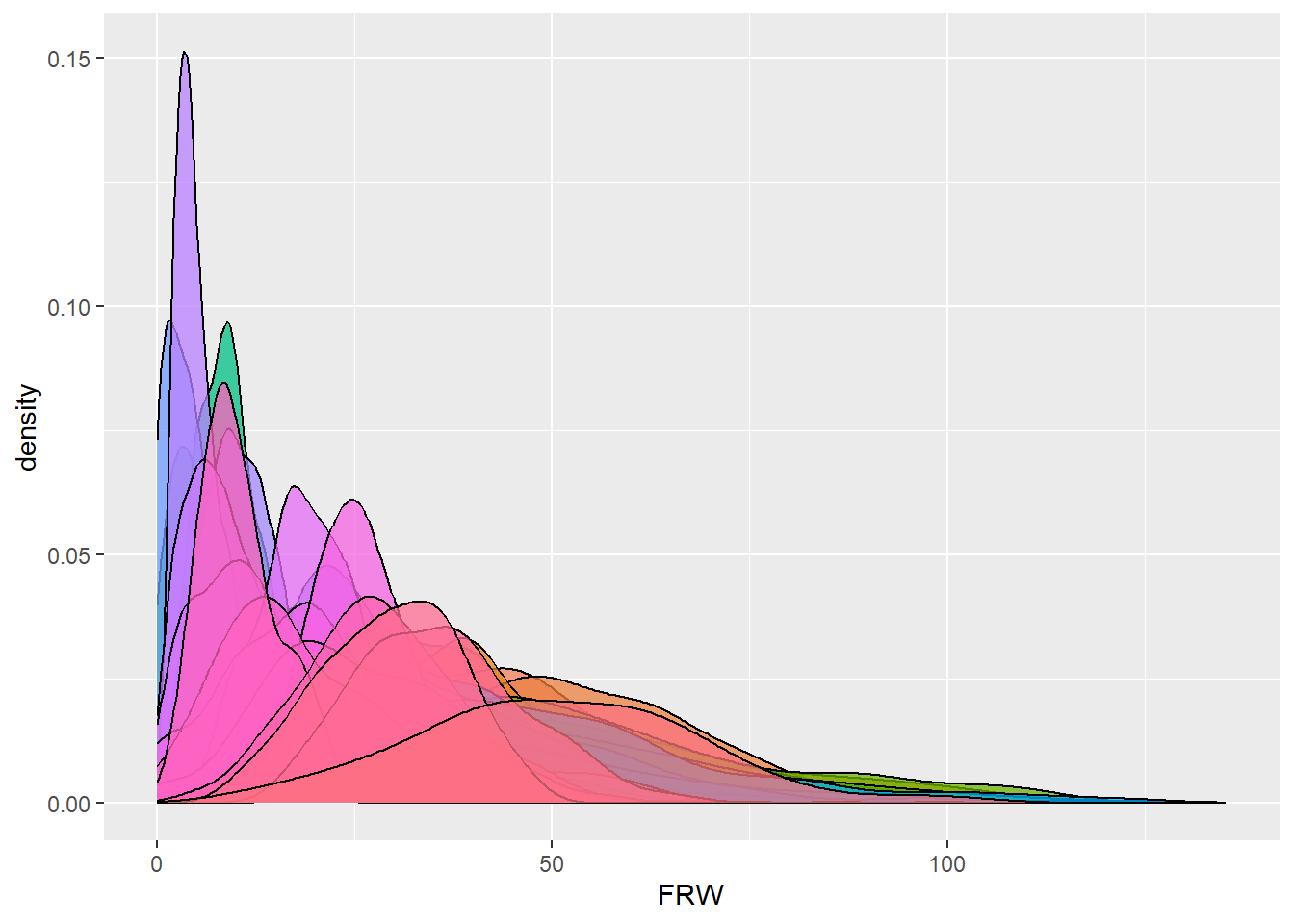

Version	Author	Date
0c01e7b	WevertonGomesCosta	2025-10-04

dbdata %>% ggplot(aes(x = FSW, fill = studyName)) + geom_density(alpha = 0.75, show.legend = FALSE)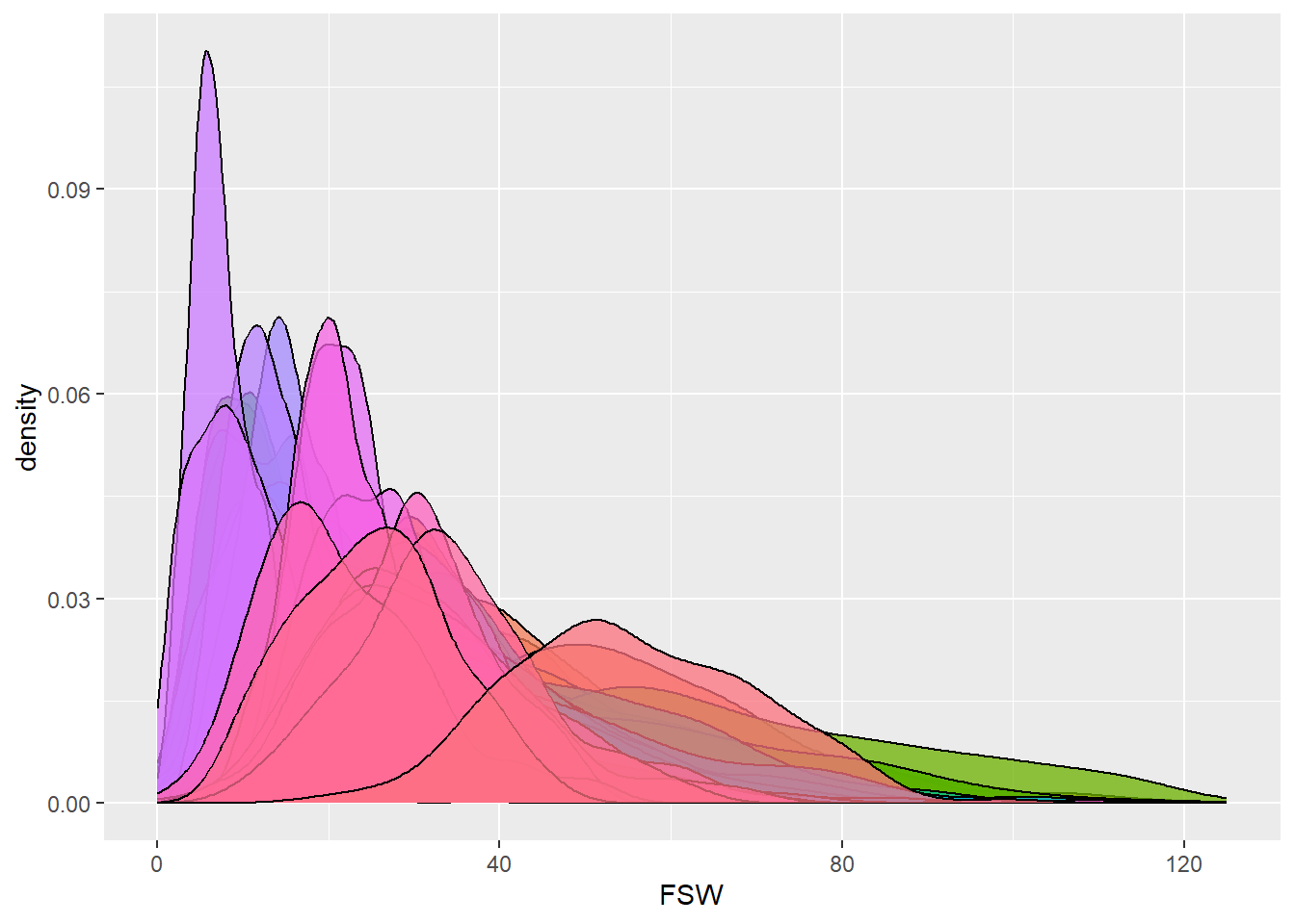

Version	Author	Date
0c01e7b	WevertonGomesCosta	2025-10-04

dbdata %>% ggplot(aes(x = DMCg, fill = studyName)) + geom_density(alpha = 0.75, show.legend = FALSE)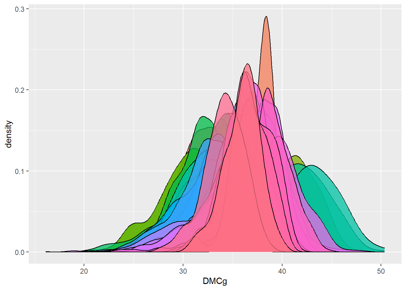

Version	Author	Date
0c01e7b	WevertonGomesCosta	2025-10-04

dbdata %>% ggplot(aes(x = DMCo, fill = studyName)) + geom_density(alpha = 0.75, show.legend = FALSE)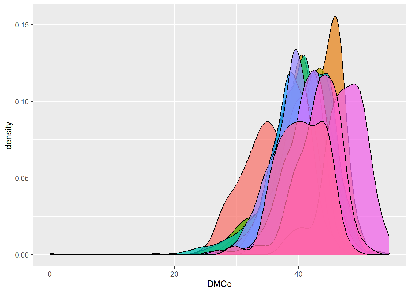

Version	Author	Date
0c01e7b	WevertonGomesCosta	2025-10-04

dbdata %>% ggplot(aes(x = StC, fill = studyName)) + geom_density(alpha = 0.75, show.legend = FALSE)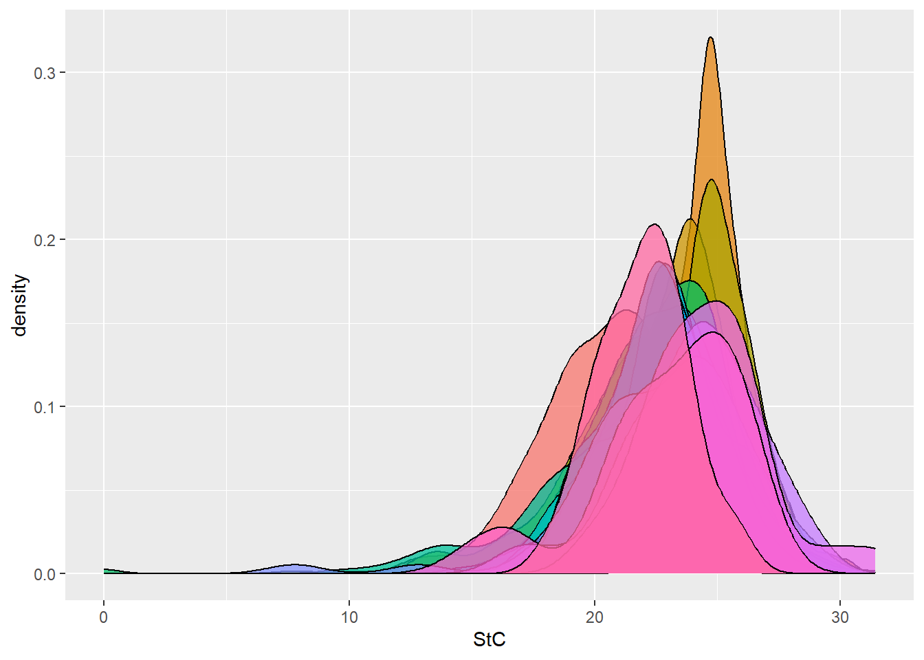

Version	Author	Date
0c01e7b	WevertonGomesCosta	2025-10-04

dbdata %>% ggplot(aes(x = PA, fill = studyName)) + geom_density(alpha = 0.75, show.legend = FALSE)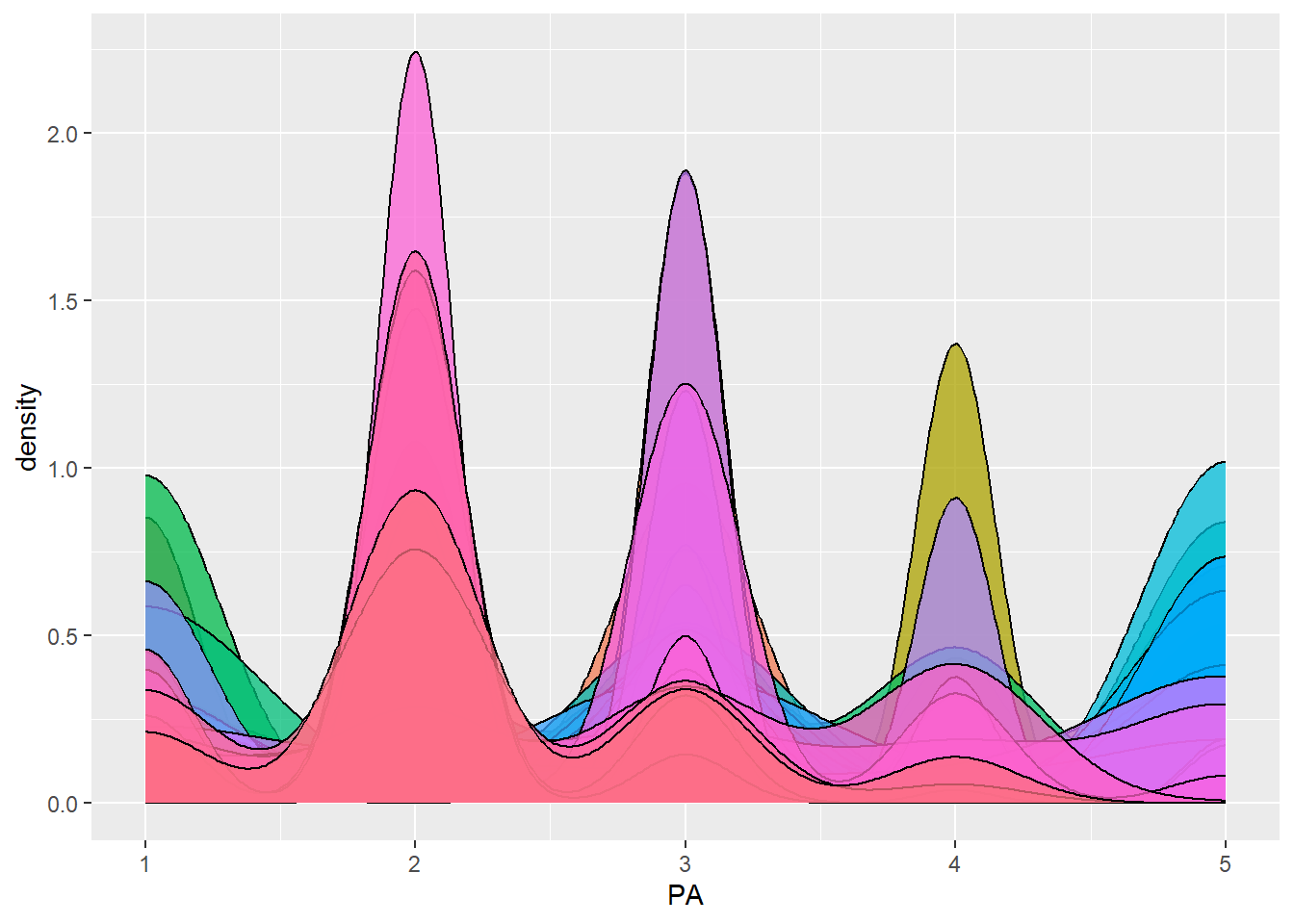

Version	Author	Date
0c01e7b	WevertonGomesCosta	2025-10-04

Interpretation:
Density plots allow us to quickly spot trials with abnormal distributions, which may indicate data entry errors or environmental effects.

Step 9: Save Cleaned Dataset

saveRDS(dbdata, file = here::here("data","phenotypes_cleaned.rds"))

Interpretation:
The cleaned dataset is saved for downstream analyses (heritability, BLUPs, selection indices). This ensures reproducibility and avoids repeating preprocessing steps.

✅ Resumo das melhorias:
- Comentários mais claros sobre cada etapa.
- Interpretações biológicas/experimentais ligadas ao programa de melhoramento.
- Estrutura narrativa que guia o leitor como um tutorial.

sessionInfo()

R version 4.5.1 (2025-06-13 ucrt)
Platform: x86_64-w64-mingw32/x64
Running under: Windows 11 x64 (build 26100)

Matrix products: default
  LAPACK version 3.12.1

locale:
[1] LC_COLLATE=Portuguese_Brazil.utf8  LC_CTYPE=Portuguese_Brazil.utf8   
[3] LC_MONETARY=Portuguese_Brazil.utf8 LC_NUMERIC=C                      
[5] LC_TIME=Portuguese_Brazil.utf8    

time zone: America/Sao_Paulo
tzcode source: internal

attached base packages:
[1] stats     graphics  grDevices utils     datasets  methods   base     

other attached packages:
 [1] genomicMateSelectR_0.2.0 data.table_1.17.8        readxl_1.4.5            
 [4] lubridate_1.9.4          forcats_1.0.0            stringr_1.5.2           
 [7] dplyr_1.1.4              purrr_1.1.0              readr_2.1.5             
[10] tidyr_1.3.1              tibble_3.3.0             ggplot2_4.0.0           
[13] tidyverse_2.0.0          gt_1.1.0                

loaded via a namespace (and not attached):
 [1] utf8_1.2.6         sass_0.4.10        generics_0.1.4     xml2_1.4.0        
 [5] stringi_1.8.7      hms_1.1.3          digest_0.6.37      magrittr_2.0.4    
 [9] timechange_0.3.0   evaluate_1.0.5     grid_4.5.1         RColorBrewer_1.1-3
[13] fastmap_1.2.0      cellranger_1.1.0   rprojroot_2.1.1    workflowr_1.7.2   
[17] jsonlite_2.0.0     whisker_0.4.1      promises_1.3.3     scales_1.4.0      
[21] jquerylib_0.1.4    cli_3.6.5          crayon_1.5.3       rlang_1.1.6       
[25] bit64_4.6.0-1      withr_3.0.2        cachem_1.1.0       yaml_2.3.10       
[29] parallel_4.5.1     tools_4.5.1        tzdb_0.5.0         httpuv_1.6.16     
[33] here_1.0.2         vctrs_0.6.5        R6_2.6.1           lifecycle_1.0.4   
[37] git2r_0.36.2       bit_4.6.0          fs_1.6.6           vroom_1.6.5       
[41] pkgconfig_2.0.3    pillar_1.11.1      bslib_0.9.0        later_1.4.4       
[45] gtable_0.3.6       glue_1.8.0         Rcpp_1.1.0         xfun_0.53         
[49] tidyselect_1.2.1   rstudioapi_0.17.1  knitr_1.50         farver_2.1.2      
[53] htmltools_0.5.8.1  labeling_0.4.3     rmarkdown_2.29     compiler_4.5.1    
[57] S7_0.2.0

Weverton Gomes da Costa, Pós-Doutorando, Embrapa Mandioca e Fruticultura, wevertonufv@gmail.com ↩︎

Phenotype Data

Costa, W. G.¹

2025-10-04

Introduction

Step 1: Loading Packages

Step 2: Defining the C0 Population

Step 3: Importing Phenotype and Metadata

Step 4: Clone Counts per Population

Step 5: Experimental Design Checks

Step 6: Replicates vs Blocks Consistency

Step 7: Nested Design Variables

Step 8: QC of Trait Values

Step 9: Save Cleaned Dataset

Phenotype Data

Costa, W. G.1

2025-10-04

Introduction

Step 1: Loading Packages

Step 2: Defining the C0 Population

Step 3: Importing Phenotype and Metadata

Step 4: Clone Counts per Population

Step 5: Experimental Design Checks

Step 6: Replicates vs Blocks Consistency

Step 7: Nested Design Variables

Step 8: QC of Trait Values

Step 9: Save Cleaned Dataset

Costa, W. G.¹