Reproducible Analysis
Last updated: 2026-07-13
Checks: 7 0
Knit directory:
nonlinear-ge-interaction-shap/
This reproducible R Markdown analysis was created with workflowr (version 1.7.2). The Checks tab describes the reproducibility checks that were applied when the results were created. The Past versions tab lists the development history.
Great! Since the R Markdown file has been committed to the Git repository, you know the exact version of the code that produced these results.
Great job! The global environment was empty. Objects defined in the global environment can affect the analysis in your R Markdown file in unknown ways. For reproduciblity it’s best to always run the code in an empty environment.
The command set.seed(20260713) was run prior to running
the code in the R Markdown file. Setting a seed ensures that any results
that rely on randomness, e.g. subsampling or permutations, are
reproducible.
Great job! Recording the operating system, R version, and package versions is critical for reproducibility.
Nice! There were no cached chunks for this analysis, so you can be confident that you successfully produced the results during this run.
Great job! Using relative paths to the files within your workflowr project makes it easier to run your code on other machines.
Great! You are using Git for version control. Tracking code development and connecting the code version to the results is critical for reproducibility.
The results in this page were generated with repository version df4cac4. See the Past versions tab to see a history of the changes made to the R Markdown and HTML files.
Note that you need to be careful to ensure that all relevant files for
the analysis have been committed to Git prior to generating the results
(you can use wflow_publish or
wflow_git_commit). workflowr only checks the R Markdown
file, but you know if there are other scripts or data files that it
depends on. Below is the status of the Git repository when the results
were generated:
Ignored files:
    Ignored:    .Rproj.user/
    Ignored:    code/Codigo_SHAP_GE_10_07_23.txt
    Ignored:    data/Manuscript_MN_NE_ACCN.docx
Note that any generated files, e.g. HTML, png, CSS, etc., are not included in this status report because it is ok for generated content to have uncommitted changes.
These are the previous versions of the repository in which changes were
made to the R Markdown (analysis/analysis.Rmd) and HTML
(docs/analysis.html) files. If you’ve configured a remote
Git repository (see ?wflow_git_remote), click on the
hyperlinks in the table below to view the files as they were in that
past version.
| File | Version | Author | Date | Message |
|---|---|---|---|---|
| Rmd | df4cac4 | WevertonGomesCosta | 2026-07-13 | Add AMMI decomposition and interaction biplot |
| html | 95e3343 | WevertonGomesCosta | 2026-07-13 | Build site. |
| Rmd | df27105 | WevertonGomesCosta | 2026-07-13 | Fix SHAP profile plot margin namespace |
| html | b59cfdd | WevertonGomesCosta | 2026-07-13 | Build site. |
| Rmd | 236dcfd | WevertonGomesCosta | 2026-07-13 | Add environmental index and Random Forest validation |
| html | 029bb27 | WevertonGomesCosta | 2026-07-13 | Build site. |
| Rmd | 3bca313 | WevertonGomesCosta | 2026-07-13 | Add data preparation and phenotypic performance analysis |
| html | 9f70394 | WevertonGomesCosta | 2026-07-13 | Build site. |
| Rmd | 6f375a8 | WevertonGomesCosta | 2026-07-13 | Add initial reproducible analysis page |
Overview
This page presents the complete reproducible analytical workflow associated with the study “Non-Linear Modeling of Genotype × Environment Interaction via Tree-Based Learning Algorithms and Shapley Decomposition.”
The workflow combines phenotypic evaluation, Random Forest modeling, Shapley Additive Explanations, AMMI decomposition, stability indices, genotype ranking, and rank correlation.
All analytical code is presented directly in this R Markdown document and follows the order required to reproduce the analysis.
knitr::opts_chunk$set(
  echo = TRUE,
  warning = FALSE,
  message = FALSE,
  fig.align = "center",
  fig.width = "100%",
  fig.height = 6
)
Required packages
The following packages are used for data manipulation, graphical visualization, Random Forest modeling, and SHAP decomposition.
library(ggplot2)
library(dplyr)
library(tidyr)
library(randomForest)
library(DALEX)
Data import
The maize multi-environment trial data set is stored as a
tab-delimited text file in the data directory.
maize <- read.table(
  "data/maize.txt",
  h = TRUE
)

head(maize)
ENV GEN REP GY
1 1 1 1 3699.7
2 1 1 2 2947.9
3 1 1 3 3745.3
4 1 1 4 4093.3
5 1 2 1 3801.2
6 1 2 2 1631.4Data preparation
The original replicate-level observations are summarized by genotype and environment. The resulting data frame contains the mean grain yield for each genotype-by-environment combination.
df_ml <- maize %>%
  group_by(GEN, ENV) %>%
  summarise(
    GY = mean(GY, na.rm = TRUE),
    .groups = "drop"
  )

df_ml$ENV <- as.factor(df_ml$ENV)
df_ml$GEN <- as.factor(df_ml$GEN)
Phenotypic performance
Grain yield across environments
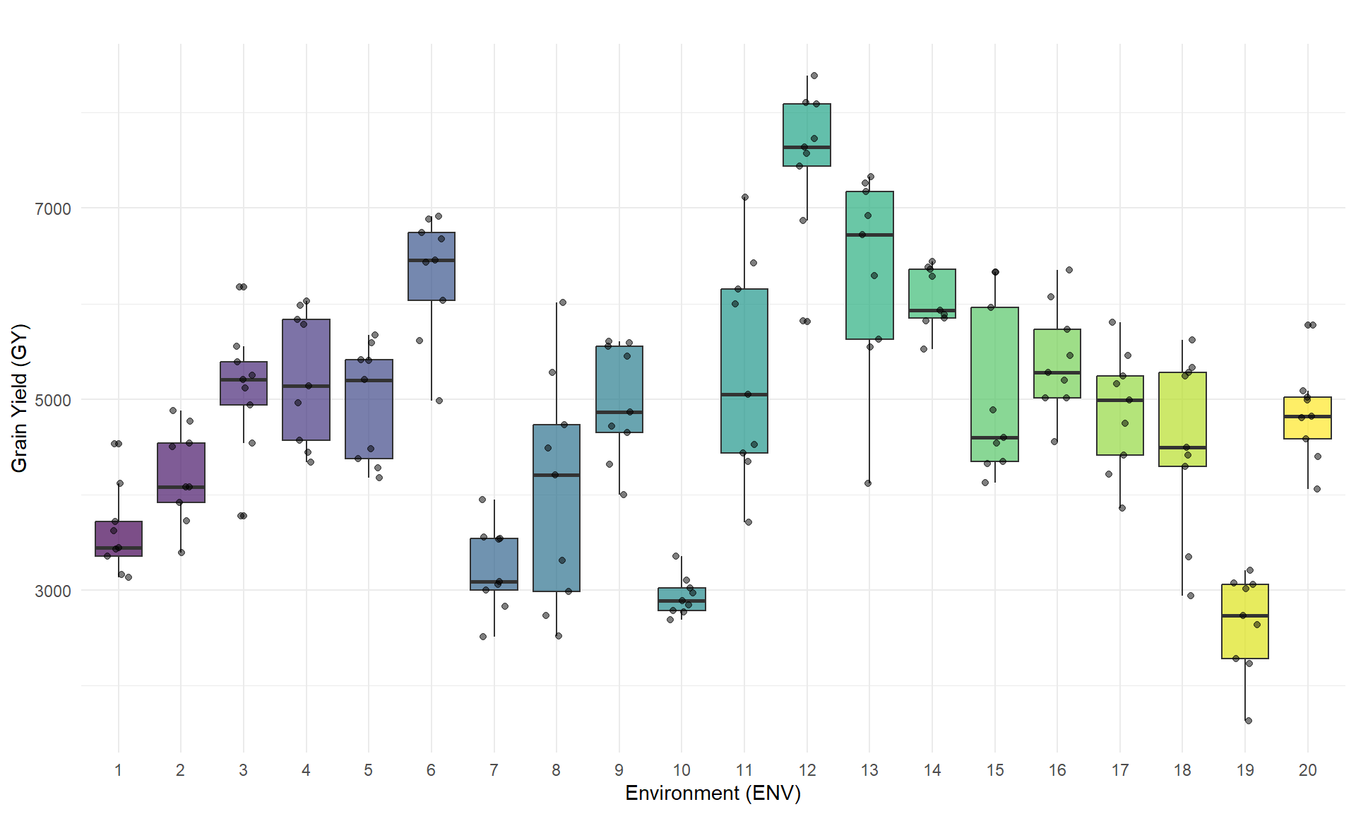
The distribution of mean grain yield is represented for each environment. Each point corresponds to the mean performance of one genotype within an environment.
ggplot(df_ml, aes(x = ENV, y = GY, fill = ENV)) +
  geom_boxplot(
    alpha = 0.7,
    show.legend = FALSE
  ) +
  geom_jitter(
    width = 0.2,
    alpha = 0.5,
    color = "black"
  ) +
  labs(
    title = "",
    x = "Environment (ENV)",
    y = "Grain Yield (GY)"
  ) +
  theme_minimal() +
  scale_fill_viridis_d() +
  theme(
    legend.position = "none"
  )
| Version | Author | Date |
|---|---|---|
| 029bb27 | WevertonGomesCosta | 2026-07-13 |
Grain yield across genotypes
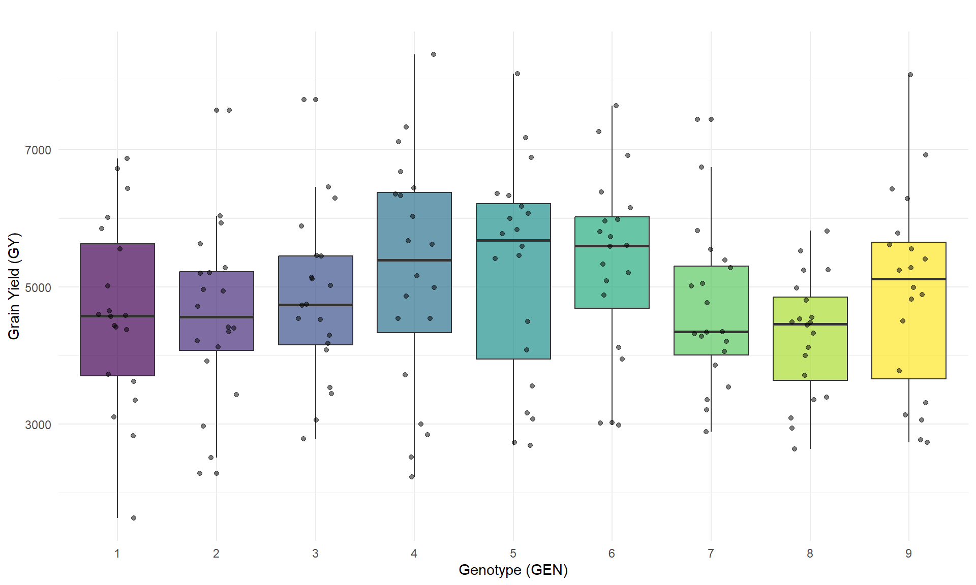
The distribution of mean grain yield is represented for each genotype. Each point corresponds to the mean performance of one genotype within an environment.
ggplot(df_ml, aes(x = GEN, y = GY, fill = GEN)) +
  geom_boxplot(
    alpha = 0.7
  ) +
  geom_jitter(
    width = 0.2,
    alpha = 0.5,
    color = "black"
  ) +
  labs(
    title = "",
    x = "Genotype (GEN)",
    y = "Grain Yield (GY)"
  ) +
  theme_minimal() +
  scale_fill_viridis_d() +
  theme(
    legend.position = "none"
  )
| Version | Author | Date |
|---|---|---|
| 029bb27 | WevertonGomesCosta | 2026-07-13 |
Environmental index
The environmental index is calculated as the mean grain yield of all genotypes evaluated within each environment. This continuous variable represents the productive potential of each environment.
env_indices <- df_ml %>%
  group_by(ENV) %>%
  summarise(
    ENV_INDEX = mean(GY, na.rm = TRUE),
    .groups = "drop"
  )

df_ml <- df_ml %>%
  left_join(env_indices, by = "ENV")

head(env_indices)
# A tibble: 6 × 2
ENV ENV_INDEX
<fct> <dbl>
1 1 3613.
2 2 4209.
3 3 5105.
4 4 5230.
5 5 4955.
6 6 6305.Random Forest modeling
Leave-one-environment-out validation
The Random Forest model is evaluated through leave-one-environment-out cross-validation. At each iteration, one environment is reserved for prediction, while the remaining environments are used for model fitting.
set.seed(42)

ambientes <- unique(df_ml$ENV)
predicoes_cv <- data.frame()

cat("Starting leave-one-environment-out cross-validation...\n")
Starting leave-one-environment-out cross-validation...for (env_teste in ambientes) {
dados_treino <- df_ml %>%
filter(ENV != env_teste)
dados_teste <- df_ml %>%
filter(ENV == env_teste)
rf_fold <- randomForest(
GY ~ GEN + ENV_INDEX,
data = dados_treino,
ntree = 500
)
dados_teste$Pred_GY <- predict(
rf_fold,
newdata = dados_teste
)
predicoes_cv <- bind_rows(
predicoes_cv,
dados_teste
)
}Predictive metrics
Predictive performance is summarized using the cross-validated coefficient of determination, the Pearson correlation between observed and predicted grain yield, and the root mean squared error.
ss_res <- sum(
  (predicoes_cv$GY - predicoes_cv$Pred_GY)^2
)

ss_tot <- sum(
  (predicoes_cv$GY - mean(predicoes_cv$GY))^2
)

r2_cv <- 1 - (ss_res / ss_tot)

rmse_cv <- sqrt(
  mean(
    (predicoes_cv$GY - predicoes_cv$Pred_GY)^2
  )
)

accuracy_r <- cor(
  predicoes_cv$GY,
  predicoes_cv$Pred_GY
)

cat(
  "\n=== LEAVE-ONE-ENVIRONMENT-OUT VALIDATION METRICS ===\n"
)
=== LEAVE-ONE-ENVIRONMENT-OUT VALIDATION METRICS ===cat(
"Predictive capacity (cross-validated R²): ",
round(r2_cv * 100, 2),
"%\n"
)Predictive capacity (cross-validated R²): 71.94 %cat(
"Predictive accuracy (r): ",
round(accuracy_r, 2),
"\n"
)Predictive accuracy (r): 0.85 cat(
"Cross-validation RMSE: ",
round(rmse_cv, 2),
" kg ha-1\n"
)Cross-validation RMSE: 717.02 kg ha-1Final Random Forest model
The final Random Forest model is fitted using the complete analytical data set. Grain yield is modeled as a function of genotype and the continuous environmental index.
set.seed(42)

rf_model <- randomForest(
  GY ~ GEN + ENV_INDEX,
  data = df_ml,
  ntree = 500
)
SHAP decomposition
Model explainer
The Random Forest model is connected to the DALEX framework using the genotype and environmental-index predictors. The response variable supplied to the explainer is the observed mean grain yield.
explainer_rf <- explain(
  model = rf_model,
  data = df_ml[, c("GEN", "ENV_INDEX")],
  y = df_ml$GY,
  label = "Random Forest GxE (Continuous)"
)
Preparation of a new explainer is initiated
-> model label : Random Forest GxE (Continuous)
-> data : 180 rows 2 cols
-> data : tibble converted into a data.frame
-> target variable : 180 values
-> predict function : yhat.randomForest will be used ( default )
-> predicted values : No value for predict function target column. ( default )
-> model_info : package randomForest , ver. 4.7.1.2 , task regression ( default )
-> predicted values : numerical, min = 2730.198 , mean = 4854.431 , max = 7394.243
-> residual function : difference between y and yhat ( default )
-> residuals : numerical, min = -1098.198 , mean = 3.706323 , max = 1576.526
A new explainer has been created! SHAP contribution values
SHAP contributions are calculated for every genotype-by-environment observation. For each observation, the mean contribution associated with genotype and environmental index is extracted from the SHAP decomposition.
shap_list <- list()

cat("Starting SHAP contribution calculation...\n")
Starting SHAP contribution calculation...for (i in 1:nrow(df_ml)) {
obs <- df_ml[i, c("GEN", "ENV_INDEX")]
shap_obs <- predict_parts(
explainer = explainer_rf,
new_observation = obs,
type = "shap",
B = 25
)
val_gen <- shap_obs %>%
filter(variable_name == "GEN") %>%
summarise(mean(contribution)) %>%
pull()
val_env <- shap_obs %>%
filter(variable_name == "ENV_INDEX") %>%
summarise(mean(contribution)) %>%
pull()
shap_list[[i]] <- data.frame(
SHAP_GEN = val_gen,
SHAP_ENV = val_env
)
}
df_shap_final <- bind_rows(shap_list)
df_results <- cbind(
df_ml,
df_shap_final
)
head(df_results) GEN ENV GY ENV_INDEX SHAP_GEN SHAP_ENV
1 1 1 3621.550 3612.531 -151.5668 -1058.48148
2 1 2 3728.325 4209.444 -201.7336 -539.92178
3 1 3 5554.025 5104.919 -225.5393 267.99268
4 1 4 4565.575 5229.997 -349.7975 237.71528
5 1 5 4379.800 4955.231 -299.3879 21.53598
6 1 6 6436.725 6305.306 -131.2397 1370.67649Genotype response profiles
Genotype-specific SHAP contributions are represented across environments. Positive and negative values indicate the direction of the genotype contribution to the Random Forest prediction relative to the model reference value.
df_results$GEN <- as.factor(df_results$GEN)
df_results$ENV <- as.factor(df_results$ENV)

p_shap <- ggplot(
  df_results,
  aes(
    x = ENV,
    y = SHAP_GEN,
    group = GEN,
    color = GEN
  )
) +
  geom_hline(
    yintercept = 0,
    linetype = "dashed",
    color = "gray60",
    linewidth = 0.4
  ) +
  geom_line(
    linewidth = 0.8,
    alpha = 0.85
  ) +
  geom_point(
    size = 2,
    alpha = 0.9
  ) +
  scale_color_viridis_d(
    option = "viridis"
  ) +
  theme_classic(
    base_size = 12
  ) +
  labs(
    title = "",
    subtitle = "",
    x = "Environments",
    y = expression(
      paste(
        "Genotype SHAP Value (G",
        times,
        "E Effect) in kg ",
        ha^-1
      )
    ),
    color = "Genotypes"
  ) +
  theme(
    plot.title = element_text(
      face = "bold",
      size = 13,
      hjust = 0
    ),
    plot.subtitle = element_text(
      size = 10,
      color = "gray30",
      margin = ggplot2::margin(b = 12)
    ),
    axis.title = element_text(
      face = "plain",
      size = 11
    ),
    axis.text = element_text(
      color = "black",
      size = 9
    ),
    legend.position = "bottom",
    legend.title = element_text(
      face = "bold",
      size = 10
    ),
    legend.text = element_text(
      size = 9
    ),
    axis.line = element_line(
      color = "black",
      linewidth = 0.5
    )
  )

print(p_shap)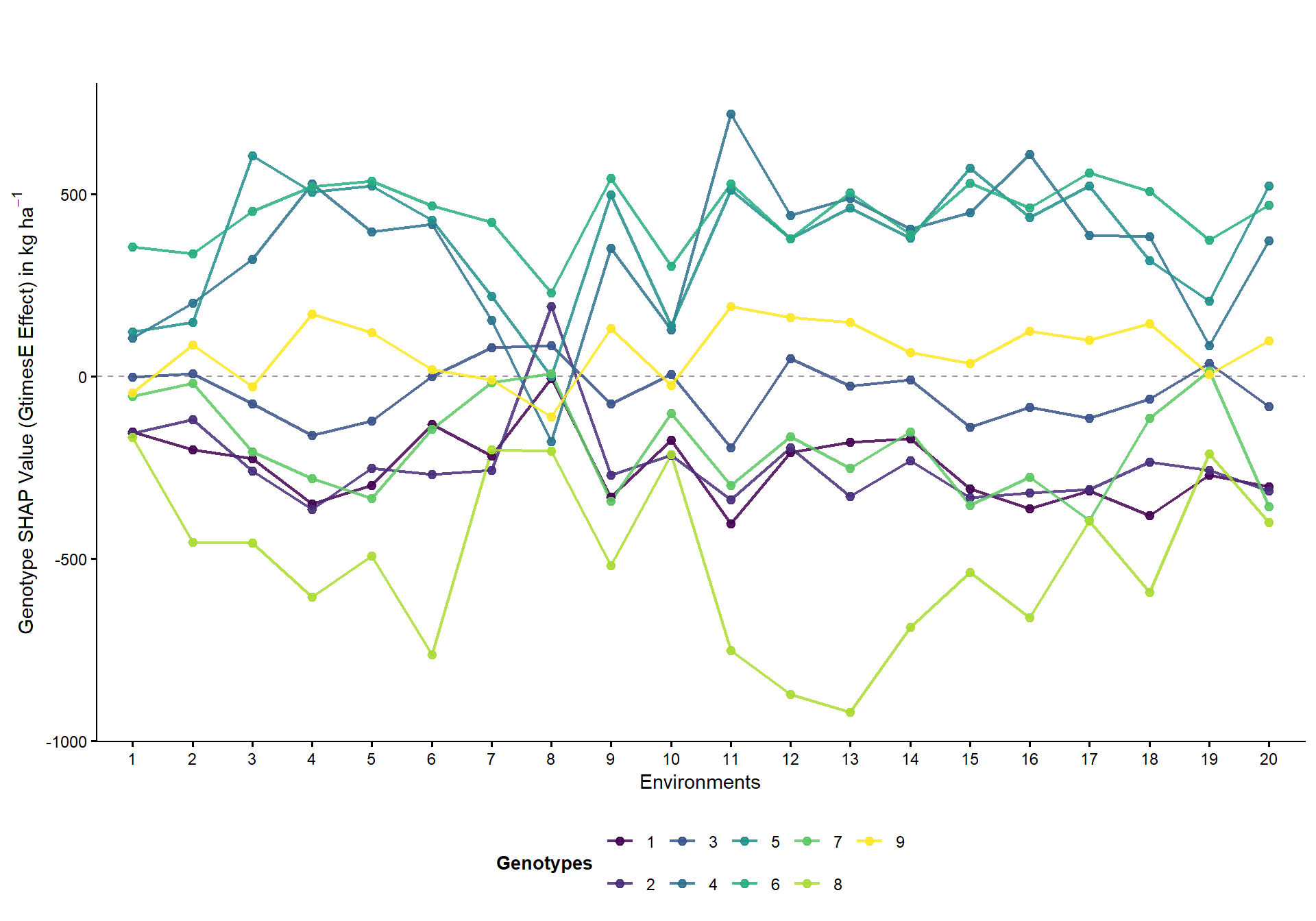
| Version | Author | Date |
|---|---|---|
| 95e3343 | WevertonGomesCosta | 2026-07-13 |
AMMI analysis
Genotype-by-environment interaction matrix
The genotype-by-environment interaction effects are obtained after removing the genotype and environment main effects from the mean grain-yield observations.
grand_mean <- mean(
  df_results$GY,
  na.rm = TRUE
)

env_effects <- df_results %>%
  group_by(ENV) %>%
  summarise(
    m_env = mean(GY, na.rm = TRUE),
    .groups = "drop"
  )

gen_effects <- df_results %>%
  group_by(GEN) %>%
  summarise(
    m_gen = mean(GY, na.rm = TRUE),
    .groups = "drop"
  )

df_int <- df_results %>%
  left_join(
    env_effects,
    by = "ENV"
  ) %>%
  left_join(
    gen_effects,
    by = "GEN"
  ) %>%
  mutate(
    GE_effect = GY - m_env - m_gen + grand_mean
  )

mat_int <- df_int %>%
  select(
    GEN,
    ENV,
    GE_effect
  ) %>%
  pivot_wider(
    names_from = ENV,
    values_from = GE_effect
  ) %>%
  tibble::column_to_rownames("GEN") %>%
  as.matrix()
Singular value decomposition
Singular value decomposition is applied to the genotype-by-environment interaction matrix. The squared singular values are used to calculate the percentage of interaction variation represented by each component.
svd_ammi <- svd(mat_int)

lambda <- svd_ammi$d

var_explained <- (
  lambda^2 / sum(lambda^2)
) * 100

ipca1_pct <- round(
  var_explained[1],
  2
)

ipca2_pct <- round(
  var_explained[2],
  2
)

data.frame(
  Component = paste0(
    "IPCA",
    seq_along(var_explained)
  ),
  Explained_variation = round(
    var_explained,
    2
  )
)
Component Explained_variation
1 IPCA1 56.20
2 IPCA2 15.10
3 IPCA3 10.44
4 IPCA4 8.62
5 IPCA5 4.95
6 IPCA6 2.76
7 IPCA7 1.01
8 IPCA8 0.92
9 IPCA9 0.00Interaction principal components
The scores of the first two interaction principal components are obtained separately for genotypes and environments.
scores_gen <- as.data.frame(
  svd_ammi$u[, 1:2] %*%
    diag(
      sqrt(lambda[1:2])
    )
)

colnames(scores_gen) <- c(
  "IPCA1",
  "IPCA2"
)

scores_gen$GEN <- as.factor(
  rownames(mat_int)
)

scores_env <- as.data.frame(
  svd_ammi$v[, 1:2] %*%
    diag(
      sqrt(lambda[1:2])
    )
)

colnames(scores_env) <- c(
  "IPCA1",
  "IPCA2"
)

scores_env$ENV <- as.factor(
  colnames(mat_int)
)
AMMI biplot
The AMMI biplot represents genotype scores and environmental vectors for the first two interaction principal components. The percentages shown on the axes correspond to the interaction variation represented by each component.
p_ammi <- ggplot() +
  geom_vline(
    xintercept = 0,
    linetype = "dashed",
    color = "gray60",
    linewidth = 0.4
  ) +
  geom_hline(
    yintercept = 0,
    linetype = "dashed",
    color = "gray60",
    linewidth = 0.4
  ) +
  geom_segment(
    data = scores_env,
    aes(
      x = 0,
      y = 0,
      xend = IPCA1,
      yend = IPCA2
    ),
    arrow = arrow(
      length = grid::unit(
        0.18,
        "cm"
      )
    ),
    color = "gray30",
    alpha = 0.6,
    linewidth = 0.5
  ) +
  geom_text(
    data = scores_env,
    aes(
      x = IPCA1,
      y = IPCA2,
      label = ENV
    ),
    vjust = 1.4,
    color = "gray20",
    size = 3
  ) +
  geom_point(
    data = scores_gen,
    aes(
      x = IPCA1,
      y = IPCA2,
      color = GEN
    ),
    size = 3.5,
    alpha = 0.9
  ) +
  geom_text(
    data = scores_gen,
    aes(
      x = IPCA1,
      y = IPCA2,
      label = GEN
    ),
    vjust = -1.2,
    fontface = "bold",
    size = 3.5,
    show.legend = FALSE
  ) +
  scale_color_viridis_d(
    option = "viridis"
  ) +
  theme_classic(
    base_size = 12
  ) +
  labs(
    x = paste0(
      "IPCA1 (",
      ipca1_pct,
      "%)"
    ),
    y = paste0(
      "IPCA2 (",
      ipca2_pct,
      "%)"
    ),
    color = "Genotypes"
  ) +
  theme(
    axis.title = element_text(
      face = "plain",
      size = 11
    ),
    axis.text = element_text(
      color = "black",
      size = 9
    ),
    axis.line = element_line(
      color = "black",
      linewidth = 0.5
    ),
    legend.position = "none"
  )

print(p_ammi)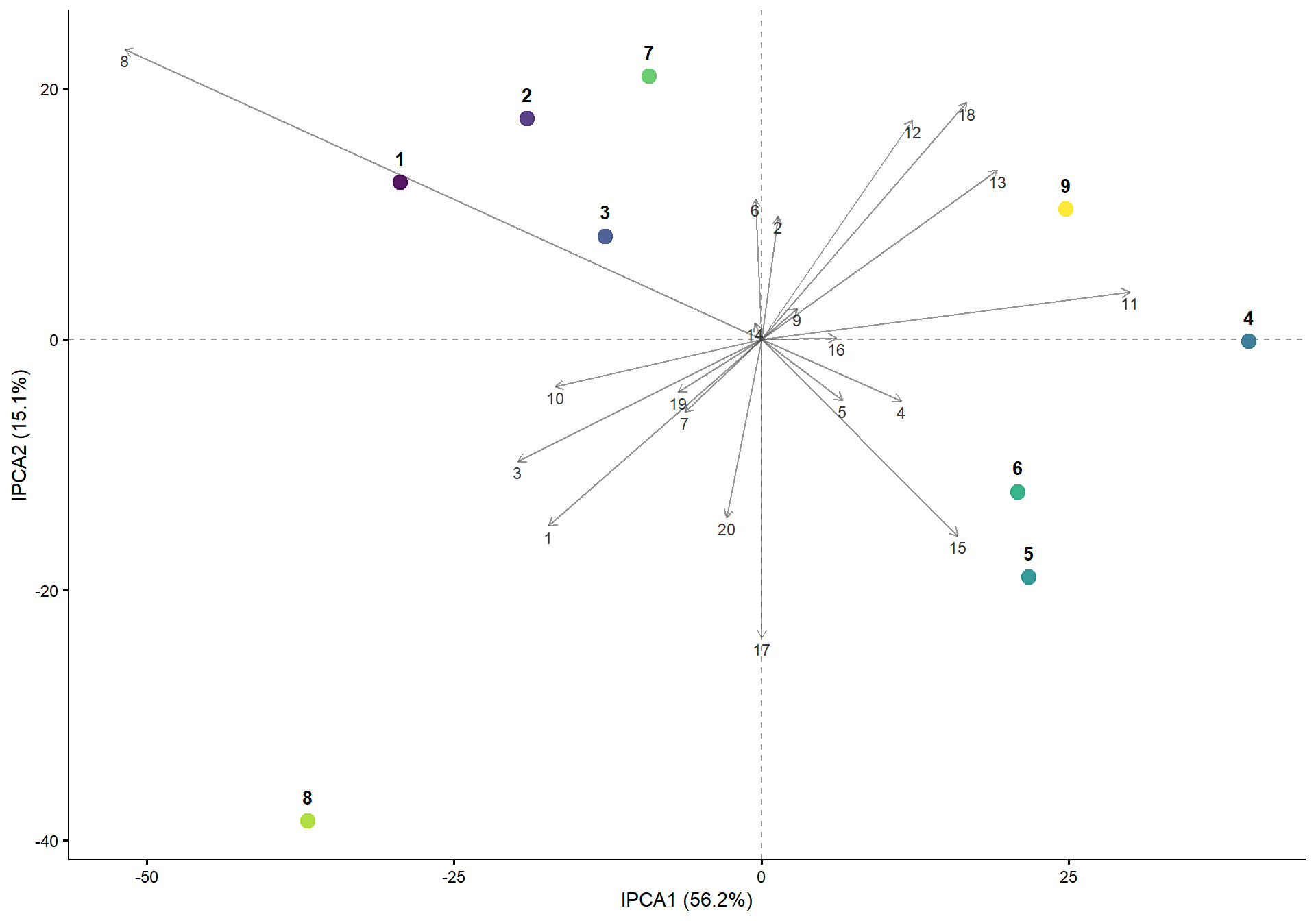
Joint AMMI and SHAP representation
The AMMI biplot and genotype SHAP profiles are combined into a single graphical representation.
Stability and selection indices
AMMI Stability Value
The AMMI Stability Value is calculated from the first two interaction principal components.
SHAP effect and stability
Mean genotype SHAP contribution and the standard deviation of genotype SHAP contributions are summarized for each genotype.
Simultaneous Selection Index
The Simultaneous Selection Index combines grain-yield and AMMI stability rankings.
Genotype ranking
Genotypes are compared according to:
- grain yield;
- AMMI Stability Value;
- Simultaneous Selection Index;
- SHAP effect;
- SHAP stability.
Rank dynamics
A bump chart represents changes in genotype positions across the evaluated criteria.
Stability concordance
The relationship between AMMI stability ranking and SHAP stability ranking is represented using a rank-concordance plot.
Spearman rank correlation
Spearman correlations are calculated among grain yield, AMMI stability, simultaneous selection, SHAP effect, and SHAP stability rankings.
sessionInfo()R version 4.5.1 (2025-06-13 ucrt)
Platform: x86_64-w64-mingw32/x64
Running under: Windows 11 x64 (build 26200)
Matrix products: default
LAPACK version 3.12.1
locale:
[1] LC_COLLATE=Portuguese_Brazil.utf8 LC_CTYPE=Portuguese_Brazil.utf8
[3] LC_MONETARY=Portuguese_Brazil.utf8 LC_NUMERIC=C
[5] LC_TIME=Portuguese_Brazil.utf8
time zone: America/Sao_Paulo
tzcode source: internal
attached base packages:
[1] stats graphics grDevices utils datasets methods base
other attached packages:
[1] DALEX_2.5.3 randomForest_4.7-1.2 tidyr_1.3.2
[4] dplyr_1.2.1 ggplot2_4.0.3 workflowr_1.7.2
loaded via a namespace (and not attached):
[1] utf8_1.2.6 sass_0.4.10 generics_0.1.4 stringi_1.8.7
[5] digest_0.6.39 magrittr_2.0.4 evaluate_1.0.5 grid_4.5.1
[9] RColorBrewer_1.1-3 fastmap_1.2.0 rprojroot_2.1.1 jsonlite_2.0.0
[13] processx_3.8.6 whisker_0.4.1 ps_1.9.1 promises_1.5.0
[17] httr_1.4.7 purrr_1.2.1 viridisLite_0.4.2 scales_1.4.0
[21] jquerylib_0.1.4 cli_3.6.5 rlang_1.1.7 iBreakDown_2.1.2
[25] withr_3.0.2 cachem_1.1.0 yaml_2.3.12 otel_0.2.0
[29] tools_4.5.1 httpuv_1.6.16 vctrs_0.7.1 R6_2.6.1
[33] lifecycle_1.0.5 git2r_0.36.2 stringr_1.6.0 fs_1.6.6
[37] pkgconfig_2.0.3 callr_3.7.6 pillar_1.11.1 bslib_0.9.0
[41] later_1.4.4 gtable_0.3.6 glue_1.8.0 Rcpp_1.1.1
[45] xfun_0.54 tibble_3.3.1 tidyselect_1.2.1 rstudioapi_0.17.1
[49] knitr_1.50 farver_2.1.2 htmltools_0.5.9 rmarkdown_2.30
[53] labeling_0.4.3 compiler_4.5.1 getPass_0.2-4 S7_0.2.1