Introduction to rmarkdown
Last updated: 2019-04-09
Checks: 6 0
Knit directory: rrresearch/
This reproducible R Markdown analysis was created with workflowr (version 1.2.0). The Report tab describes the reproducibility checks that were applied when the results were created. The Past versions tab lists the development history.
Great! Since the R Markdown file has been committed to the Git repository, you know the exact version of the code that produced these results.
Great job! The global environment was empty. Objects defined in the global environment can affect the analysis in your R Markdown file in unknown ways. For reproduciblity it’s best to always run the code in an empty environment.
The command set.seed(20190216) was run prior to running the code in the R Markdown file. Setting a seed ensures that any results that rely on randomness, e.g. subsampling or permutations, are reproducible.
Great job! Recording the operating system, R version, and package versions is critical for reproducibility.
Nice! There were no cached chunks for this analysis, so you can be confident that you successfully produced the results during this run.
Great! You are using Git for version control. Tracking code development and connecting the code version to the results is critical for reproducibility. The version displayed above was the version of the Git repository at the time these results were generated.
Note that you need to be careful to ensure that all relevant files for the analysis have been committed to Git prior to generating the results (you can use wflow_publish or wflow_git_commit). workflowr only checks the R Markdown file, but you know if there are other scripts or data files that it depends on. Below is the status of the Git repository when the results were generated:
Ignored files:
    Ignored:    .DS_Store
    Ignored:    .Rhistory
    Ignored:    .Rproj.user/
    Ignored:    analysis/.DS_Store
    Ignored:    analysis/assets/
    Ignored:    assets/
    Ignored:    data/metadata/
    Ignored:    data/raw/
    Ignored:    demos/demo-rmd-0_files/
    Ignored:    demos/demo-rmd-1_files/
    Ignored:    demos/demo-rmd_files/
    Ignored:    docs/.DS_Store
    Ignored:    docs/assets/.DS_Store
    Ignored:    docs/assets/img/.DS_Store
    Ignored:    docs/demo-rmd-0_files/
    Ignored:    docs/demo-rmd-1_files/
    Ignored:    docs/demo-rmd-2_files/
    Ignored:    docs/demo-rmd-3_files/
    Ignored:    docs/demo-rmd_files/
    Ignored:    docs/index-demo-pre_files/
    Ignored:    figure/
    Ignored:    install.R
    Ignored:    rmd/
    Ignored:    slides/libs/

Unstaged changes:
    Modified:   render-other.R
Note that any generated files, e.g. HTML, png, CSS, etc., are not included in this status report because it is ok for generated content to have uncommitted changes.
These are the previous versions of the R Markdown and HTML files. If you’ve configured a remote Git repository (see ?wflow_git_remote), click on the hyperlinks in the table below to view them.
| File | Version | Author | Date | Message |
|---|---|---|---|---|
| html | cd7663f | Anna Krystalli | 2019-04-09 | update site yml |
| Rmd | 329c4d5 | Anna Krystalli | 2019-04-09 | remove webshot |
| html | 00ad4f1 | Anna Krystalli | 2019-04-09 | update docs |
| Rmd | 4045cba | Anna Krystalli | 2019-04-09 | reduce dependencies |
| html | 7291335 | Anna Krystalli | 2019-04-09 | change assets url |
| html | 74ffa63 | Anna Krystalli | 2019-04-09 | commit site |
| html | 558735a | Anna Krystalli | 2019-04-09 | commit draft docs |
Literate programming
Programming paradigm first introduced by Donald E. Knuth.
Treat program as a literature understandable to human beings
move away from writing programs in the manner and order imposed by the computer
focus instead on the logic and flow of human thought and understanding
single document to integrate data analysis (executable code) with textual documentation, linking data, code, and text
Why is this important in science:
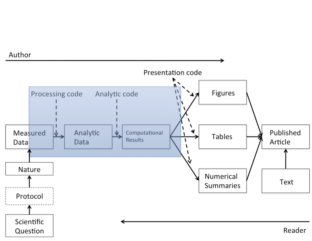
Calls for reproducibility
Reproducibility has the potential to serve as a minimum standard for judging scientific claims when full independent replication of a study is not possible.
- Fully scripted analyses pipelines
- from raw data to published tables and figures
- Publication of code and data
Calls for open science
… highlight problems with users jumping straight into software implementations of methods (e.g. in r) that may lack documentation on biases and assumptions that are mentioned in the original papers.
To help solve these problems, we make a number of suggestions including providing blog posts or videos to explain new methods in less technical terms, encouraging reproducibility and code sharing, making wiki-style pages summarising the literature on popular methods, more careful consideration and testing of whether a method is appropriate for a given question/data set, increased collaboration, and a shift from publishing purely novel methods to publishing improvements to existing methods and ways of detecting biases or testing model fit. Many of these points are applicable across methods in ecology and evolution, not just phylogenetic comparative methods.
tl;dr
- Modern open source technologies have given us great power
- With great power comes great responsibility
- You can share some of that burden by using these tools to open your work up to feedback and contribution by others. The more eyes the better.
- Use them to provide and context around your work. Help more humans understand
Literate programming in R
rmarkdown (.Rmd) integrates:
– a documentantion language (.md)
– a programming language (R)
Combine tools, processes and outputs into interactive evidence streams that are easily shareable, particularly through the web.
Rmarkdown overview
The researchers perspective
a reproducible workflow in action
elements of R markdown
markdown {.md}
stripped down html. User can focus on communicating & disseminating
intended to be as easy-to-read and easy-to-write as possible.
most powerful as a format for writing to the web.
syntax is very small, corresponding only to a very small subset of HTML tags.
clean and legible across platforms (even mobile) and outputs.
formatting handled automatically
html markup language also handled.
code {r, python, SQL, … }
Code chunks defined through special notation. Executed in sequence. Exceution of individual chunks controllable
- Analysis self-contained and reproducible
- Run in a fresh R session every time document is knit.
- A number of Language Engines are supported by
knitr- R (default)
- Python
- SQL
- Bash
- Rcpp
- Stan
- JavaScript
- CSS
Can read appropriately annotated
.Rscripts in and call them within an.Rmd
outputs
Knit together through package knitr to
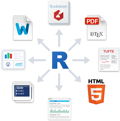
Many great packages and applications build on rmarkdown.
All this makes it incredibly versatile. Check out the gallery.
Superpower: Simple interface to powerful modern web technologies and libraries

Publish to the web for free!
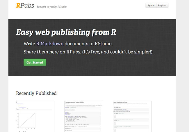
RPubs: Publish rendered rmarkdown documents on the web with the click of a button http://rpubs.com/
GitHub: Host your site through gh-pages on GitHub. Can host entire websites, like this course material https://github.com/
Applications in research
Rmd documents
Can be useful for a number of research related materials
- Vignettes: long form documentation.
- Analyses
- Documentation (code & data)
- Supplementary materials
- Reports
- Papers
Useful features: - bibliographies and citations
💻 Exercise Part 1
Throughout this workshop, we’ll be working with the gapminder dataset to produce a reproducible Rmarkdown vignette of our work. We’ll also be working in a project and setting our analysis report up to be shared online!
install the packages we’ll need
Create new project gapminder-analysis
Create your first .Rmd!
Save as index.Rmd
- Before knitting, the document needs to be saved. Give it a useful name, e.g.
index.Rmd
Render it
- Render the document by clicking on the knit button.
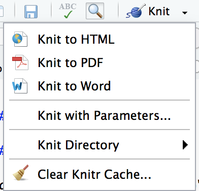
You can also render .Rmd documents to html using rmarkdown function render()
Publish your .Rmd
Register an account on RPubs
Publish your rendered document (don’t worry, you can delete or overwrite it later)
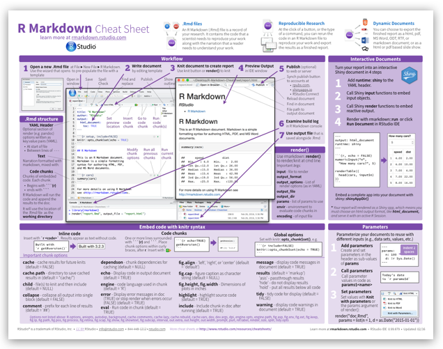
open the cheatsheet
🚦 YAML header
https://bookdown.org/yihui/rmarkdown/markdown-syntax.html
The yaml header contains metadata about the document, most importantly the output. Different seetings can be set within different outputs. Here we’ll be focusing on on the html_document output.
It is contained between these separators at the top of the file.
---

---
Markdown was originally designed for HTML output, so it may not be surprising that the HTML format has the richest features among all output formats.
define outputs
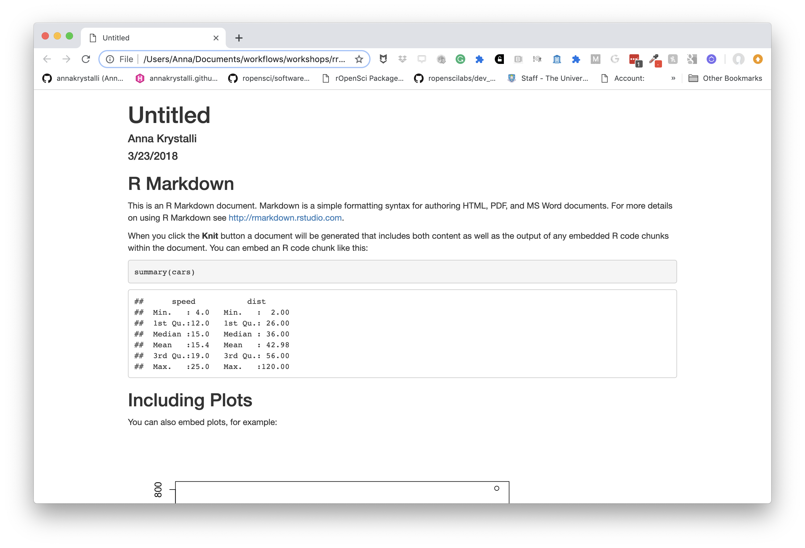
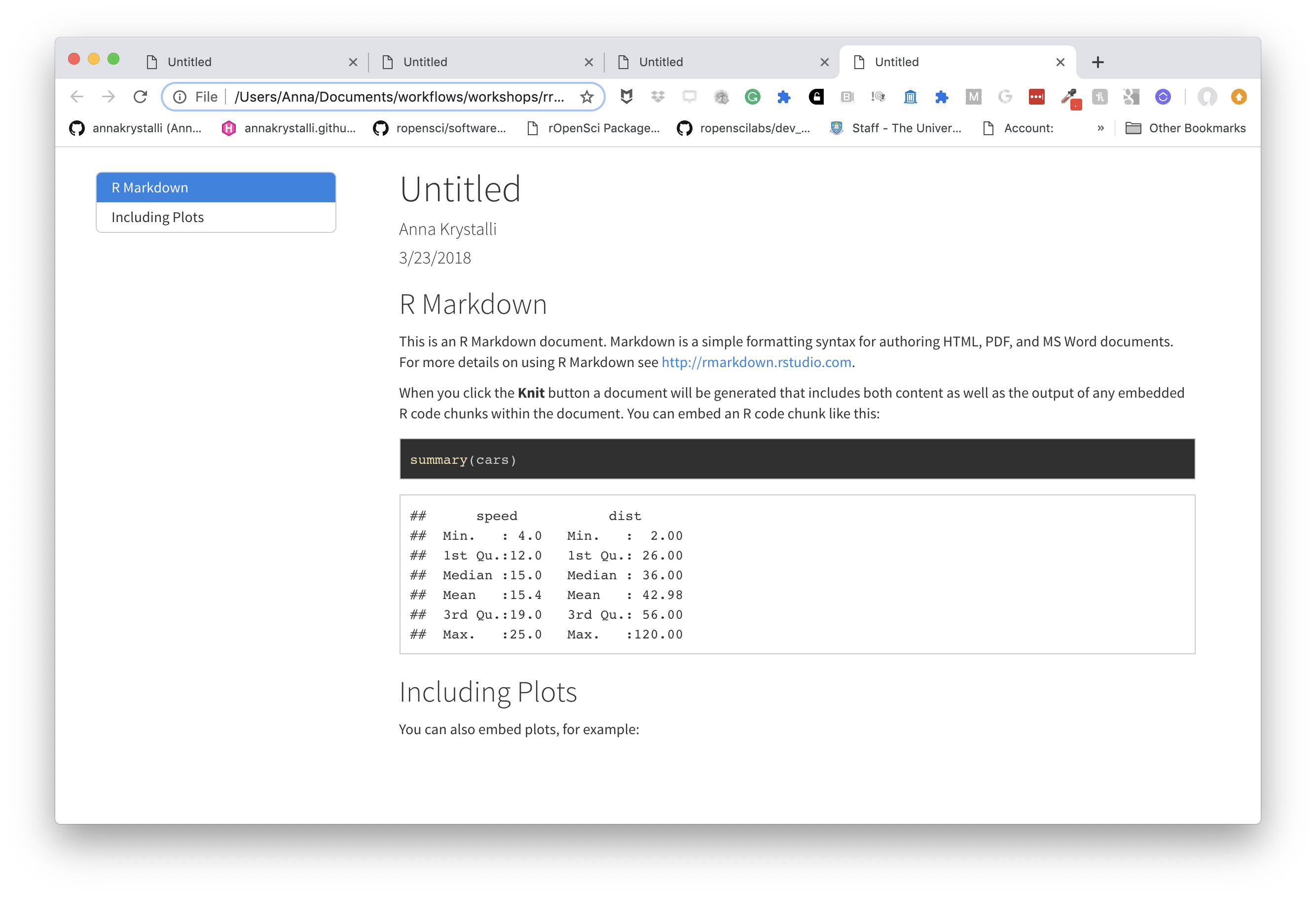
To create an HTML document from R Markdown, you specify the html_document output format in the YAML metadata of your document:
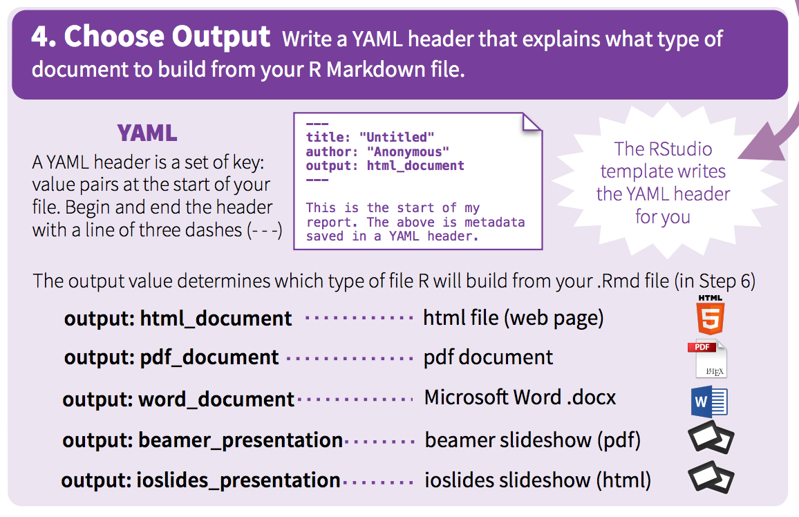
basic html_document
---
title: "Untitled"
author: "Anna Krystalli"
date: "3/23/2018"
output: html_document
---
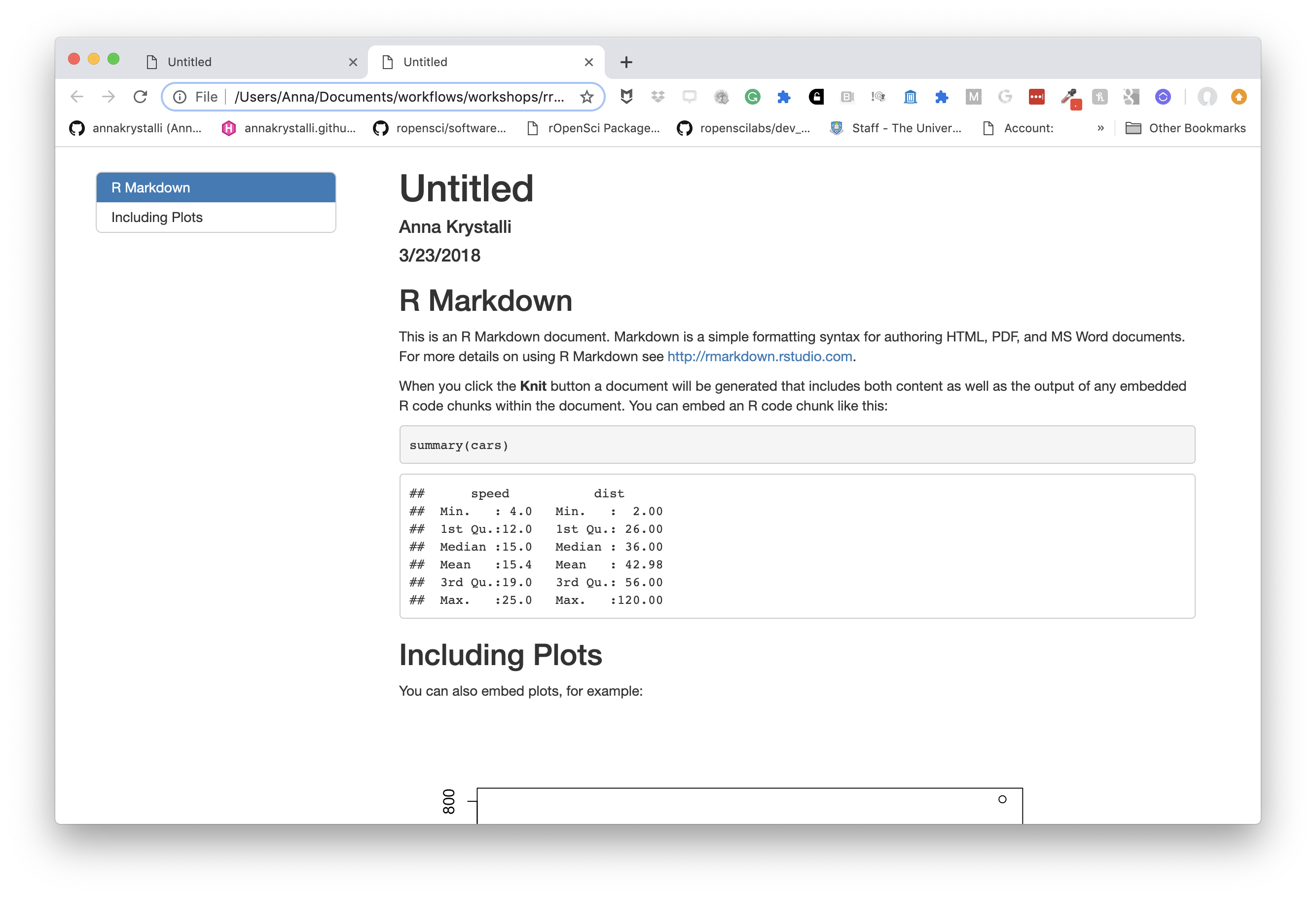
define a floating table of contents
You can add a table of contents (TOC) using the toc option and specify a floating toc using the toc_float option. For example:
---
title: "Untitled"
author: "Anna Krystalli"
date: "3/23/2018"
output:
  html_document:
    toc: true
    toc_float: true
---
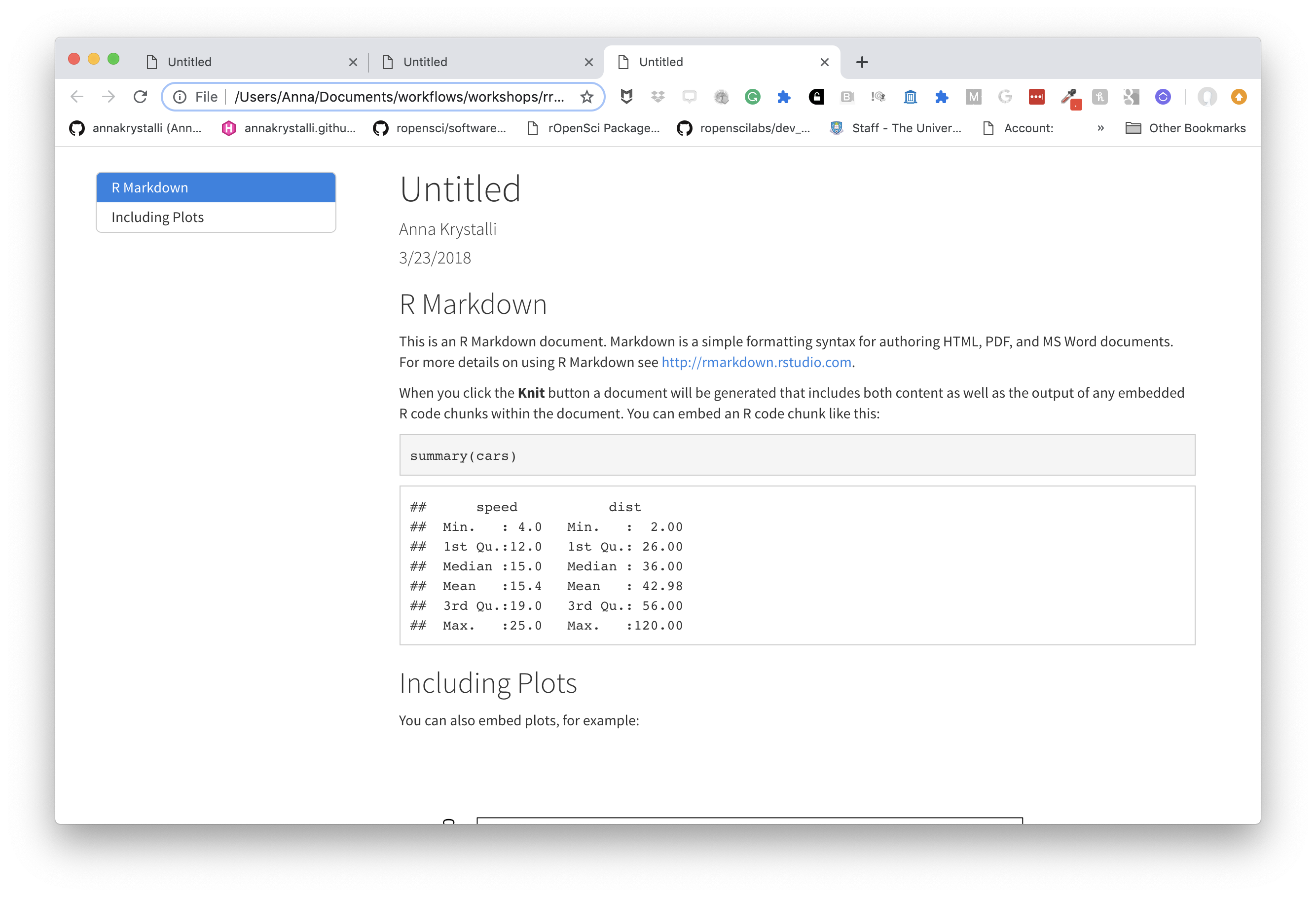
choose a theme
There are several options that control the appearance of HTML documents:
themespecifies the Bootstrap theme to use for the page (themes are drawn from the Bootswatch theme library). Valid themes includedefault,cerulean,journal,flatly,darkly,readable,spacelab,united,cosmo,lumen,paper,sandstone,simplex, andyeti.
---
title: "Untitled"
author: "Anna Krystalli"
date: "3/23/2018"
output:
  html_document:
    toc: true
    toc_float: true
    theme: cosmo
---
choose code highlights
highlight specifies the syntax highlighting style. Supported styles include default, tango, pygments, kate, monochrome, espresso, zenburn, haddock, and textmate.
---
title: "Untitled"
author: "Anna Krystalli"
date: "3/23/2018"
output:
  html_document:
    toc: true
    toc_float: true
    theme: cosmo
    highlights: zenburn
---
💻 Exercise Part 2
Clear everything BELOW THE YAML header. You should be left with just this:
---
title: "Gapminder Analysis"
author: "Anna Krystalli"
date: "3/23/2018"
output: html_document
---
add a floating table of contents
set a theme of your choice (see avalable themes here and the associated bootstrap styles here)
🚦 Markdown basics
The text in an R Markdown document is written with the Markdown syntax. Precisely speaking, it is Pandoc’s Markdown.
text
normal textnormal text
*italic text*italic text
**bold text**bold text
***bold italic text***bold italic text
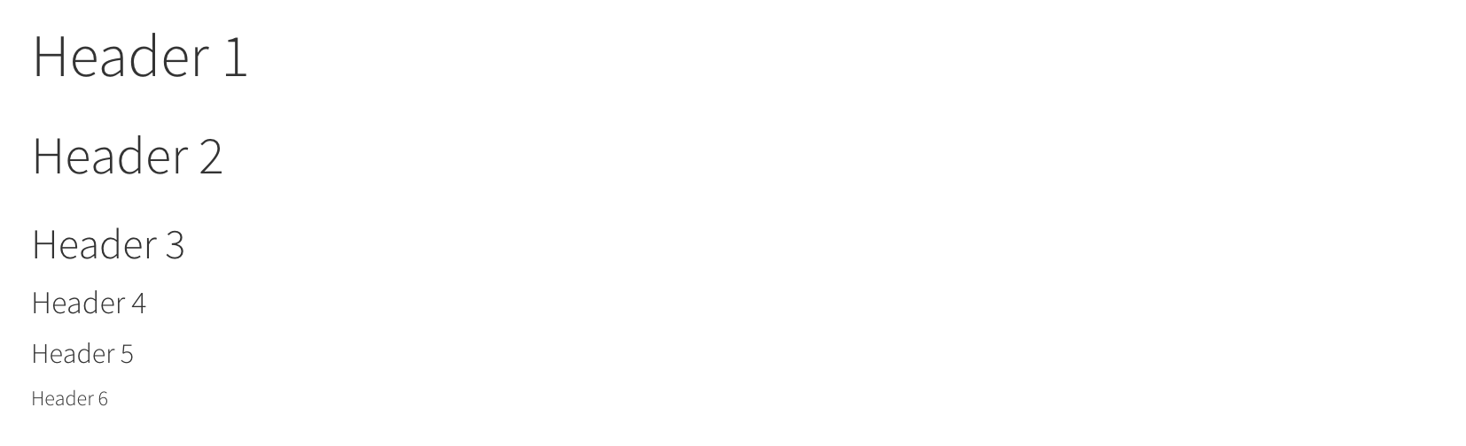
headers
rmarkdown
# Header 1
## Header 2
### Header 3
#### Header 4
##### Header 5
###### Header 6
rendered html
unordered lists
rmarkdown
- first item in the list
- second item in list
- third item in list
rendered html
- first item in the list
- second item in list
- third item in list
ordered lists
rmarkdown
1. first item in the list
1. second item in list
1. third item in list
rendered html
- first item in the list
- second item in list
- third item in list
quotes
rmarkdown
> this text will be quotedrendered html
this text will be quoted
code
annotate code inline
rmarkdown
`this text will appear as code` inlinerendered html
this text will appear as code inline
evaluate r code inline
rmarkdown
the value of parameter *a* is `r a`
rendered html
the value of parameter a is 10
images
Provide either a path to a local image file or the URL of an image.
rmarkdown

rendered html
resize images
html in rmarkdown
<img src="assets/cheat.png" width="200px" />rendered html
basic tables in markdown
rmarkdown
    Table Header  | Second Header
    ------------- | -------------
    Cell 1        | Cell 2
    Cell 3        | Cell 4
rendered html
| Table Header | Second Header |
|---|---|
| Cell 1 | Cell 2 |
| Cell 3 | Cell 4 |
Check out handy online .md table converter
links
rmarkdown
[Download R](http://www.r-project.org/)
[RStudio](http://www.rstudio.com/)
rendered html
mathematical expressions
Supports mathematical notations through MathJax.
You can write LaTeX math expressions inside a pair of dollar signs, e.g. $\alpha+\beta$ renders \(\alpha+\beta\). You can use the display style with double dollar signs:
$$\bar{X}=\frac{1}{n}\sum_{i=1}^nX_i$$\[\bar{X}=\frac{1}{n}\sum_{i=1}^nX_i\]
💻 Exercise: Part 3
Get more info on gapminder:
Do some quick online research on Gapminder. A good places to start: https://www.gapminder.org/
Create a "Background" section using headers
Write a short description
Write a short description of the Gapminder project (feel free to copy, paste and edit information). Have a look at the gapminder site and especially the about page.
Make use of markdown annotation to:
- highlight important information
- include links to sources or further information.
Add an image
Add an image related to Gapminder.
- have a look online for an image.
- include the source URL underneath for attribution.
- see if you can resize it.
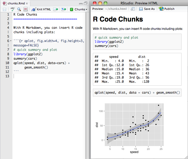
🚦 Chunks & Inline R code
inserting new chunks
You can quickly insert an R code chunk with:
- the keyboard shortcut
Ctrl + Alt + I(OS X:Cmd + Option + I) - the Add Chunk
 command in the RStudio toolbar
 - by typing the chunk delimiters
```{r} and ```.
chunk uses
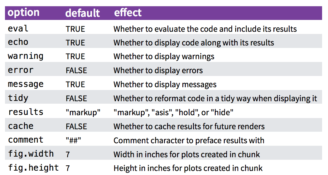
There are a lot of things you can do in a code chunk:
- you can produce text output, tables, or graphics.
- You have fine control over all these output via chunk options, which can be provided inside the curly braces (between
```{rand}).- For example, you can choose hide text output via the chunk option
results = 'hide', or set the figure height to 4 inches viafig.height = 4.
- For example, you can choose hide text output via the chunk option
- Chunk options are separated by commas, e.g.,
R code chunks execute code.
They can be used as a means to render R output into documents or to simply display code for illustration (eg with option eval=FALSE).
chunk notation
chunk notation in .rmd
```{r chunk-name}
print('hello world!')
```
rendered html code and output
[1] "hello world!"Chunks can be labelled with chunk names, names must be unique.
uses
- controlling whether code is displayed inline (
echosetting) - controlling whether code is evaluated (
evalsetting) - controlling how figures are displayed (
fig.widthandfig.heightsettings) - suppressing warnings and messages (
warningandmessagesettings) - cacheing computations (
cachesetting) - controlling whether code is extracted when using purl (
purlsettings)
controlling code display with echo
chunk notation in .rmd
```{r hide-code, echo=FALSE}
print('hello world!')
```
rendered html code and output
[1] "hello world!"controlling code evaluation with eval
chunk notation in .rmd
```{r dont-eval, eval=FALSE}
print('hello world!')
```
rendered html code and output
💻 Exercise Part 4
For this exercise we’ll be accessing the gapminder data through the gapminder R package.
Create an “Installation” section using headers
Write installation instruction
Write brief instructions (including code) for others to access the dataset in R. Have a look at the package documentation on GitHub for inspiration.
In R we often need to describe a setup proceedure that involves specifying the installation of required packages. However, installation of packages in not handled in .Rmd! (For the moment, install packages through the console).
In our case, we’ll want to include the code for installing the gapminder package but not evaluate it in the .Rmd. We also want to include the rest of the packages we want to use: “ggplot2”, “DT”, “skimr”
🚦 Displaying data
There are many ways you can display data and data properties in an .Rmd.
printing data.frames
  Ozone Solar.R Wind Temp Month Day
1    41     190  7.4   67     5   1
2    36     118  8.0   72     5   2
3    12     149 12.6   74     5   3
4    18     313 11.5   62     5   4
5    NA      NA 14.3   56     5   5
6    28      NA 14.9   66     5   6
printing tibbles
One nice feature of using tibbles over data.frames is the tidy printing behaviour:
# A tibble: 153 x 6
   Ozone Solar.R  Wind  Temp Month   Day
   <int>   <int> <dbl> <int> <int> <int>
 1    41     190   7.4    67     5     1
 2    36     118   8      72     5     2
 3    12     149  12.6    74     5     3
 4    18     313  11.5    62     5     4
 5    NA      NA  14.3    56     5     5
 6    28      NA  14.9    66     5     6
 7    23     299   8.6    65     5     7
 8    19      99  13.8    59     5     8
 9     8      19  20.1    61     5     9
10    NA     194   8.6    69     5    10
# … with 143 more rows
Displaying knitr::kable() tables
We can use other packages to create html tables from our data.
The simplest is to use the knitr::kable() function.
library(knitr)
data(airquality)
kable(head(airquality), caption = "New York Air Quality Measurements")| Ozone | Solar.R | Wind | Temp | Month | Day |
|---|---|---|---|---|---|
| 41 | 190 | 7.4 | 67 | 5 | 1 |
| 36 | 118 | 8.0 | 72 | 5 | 2 |
| 12 | 149 | 12.6 | 74 | 5 | 3 |
| 18 | 313 | 11.5 | 62 | 5 | 4 |
| NA | NA | 14.3 | 56 | 5 | 5 |
| 28 | NA | 14.9 | 66 | 5 | 6 |
Displaying interactive DT::datatable() tables
You can display interactive html tables using function DT::datatable():
Summarising data with skimr::skim()
Fuction skimr::skim() provides a simple approach to displaying summary statistics that can be quickly skimmed quickly to understand data.
Skim summary statistics
 n obs: 153
 n variables: 6

── Variable type:integer ──────────────────────────────────────────────
 variable missing complete   n   mean    sd p0    p25   p50    p75 p100
      Day       0      153 153  15.8   8.86  1   8     16    23      31
    Month       0      153 153   6.99  1.42  5   6      7     8       9
    Ozone      37      116 153  42.13 32.99  1  18     31.5  63.25  168
  Solar.R       7      146 153 185.93 90.06  7 115.75 205   258.75  334
     Temp       0      153 153  77.88  9.47 56  72     79    85      97
     hist
 ▇▇▇▇▆▇▇▇
 ▇▇▁▇▁▇▁▇
 ▇▆▃▃▂▁▁▁
 ▃▃▃▃▅▇▇▃
 ▂▂▃▆▇▇▃▃

── Variable type:numeric ──────────────────────────────────────────────
 variable missing complete   n  mean   sd  p0 p25 p50  p75 p100     hist
     Wind       0      153 153  9.96 3.52 1.7 7.4 9.7 11.5 20.7 ▁▃▇▇▅▅▁▁
💻 Exercise Part 5
Start a new section called "Dataset"
Display an example of the dataset
Make the gapminder data available by loading the gapminder package
Write a short description of the dataset
- What size is the data? (How many variables? How many rows of data points. See if you can extract and include such info inline)
- what type of object is it? (see
?class) - Use some of the functions you’ve learnt to extract such information (eg
?dim,?ncoletc).
Summarise the data
(e.g. ?summary, ?skimr)
🚦 plots
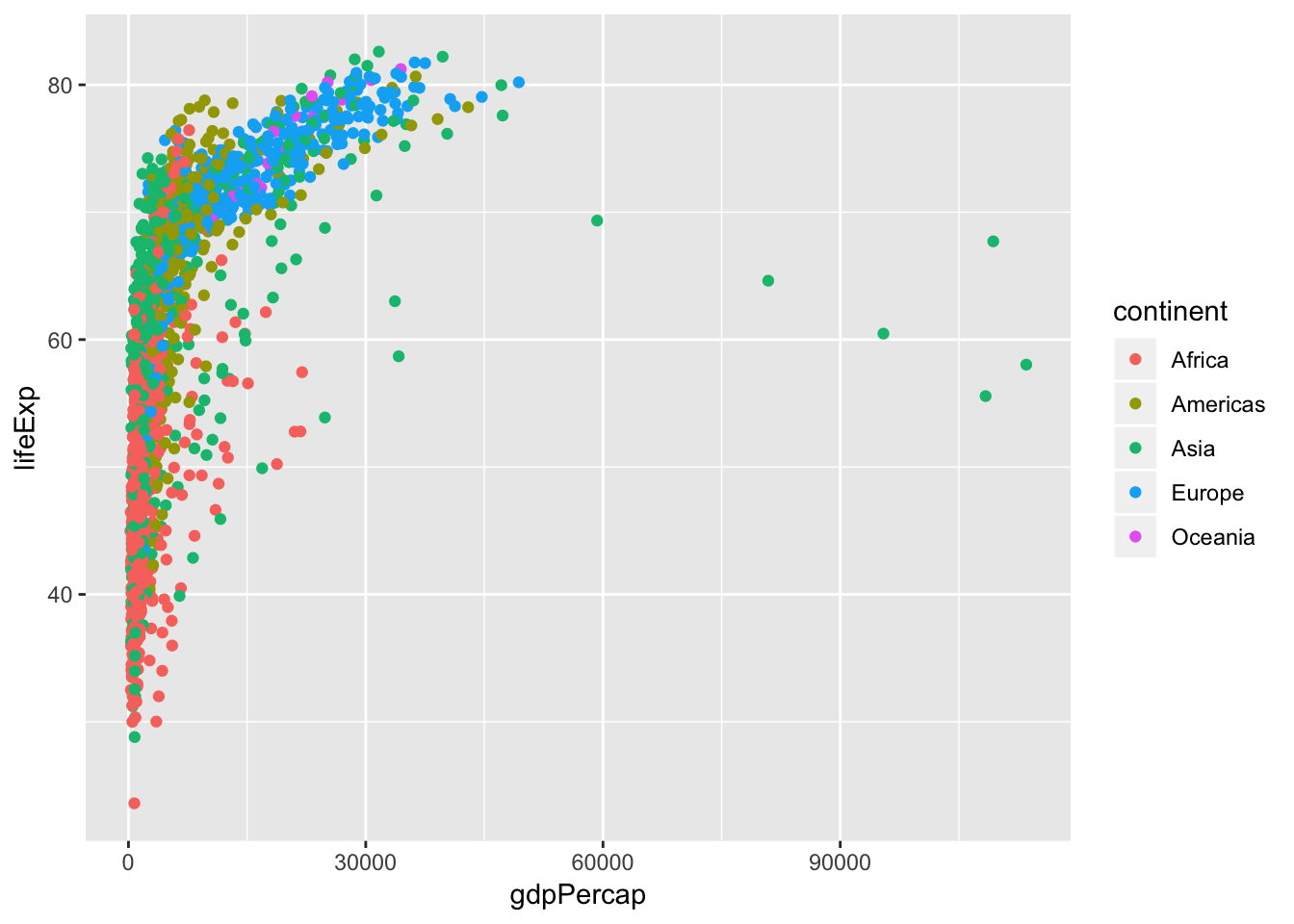
By default, figures produced by R code will be placed immediately after the code chunk they were generated from.
Let’s use ggplot2 to have a look to the relationship between a couple of variables.
| Version | Author | Date |
|---|---|---|
| c3260c9 | Anna Krystalli | 2019-04-09 |
💻 Exercise Part 6a
Replicate the plot above in your own
index.Rmdbut hide the code that generates them.Add a caption
Experiment with controlling figure output width
- OPTIONAL Can you adapt the plotting code to use log10 transformed data?
- hint: explore the
scale_...functions inggplot2(cheatsheet)
- hint: explore the
Details on chunk arguments related to plotting
🚦 Advanced .Rmd
reading chunks of code
R -> Rmd
You can read in chunks of code from an annotated .R (or any other language) script using knitr::read_chunks()
Chunks are defined by the following notation. Names must be unique.
# ---- descriptive-chunk-name1 ----
code("you want to run as a chunk")

# ---- descriptive-chunk-name2 ----
code("you want to run as a chunk")
code in .R script hello-world.R
hello-world.R
# ---- demo-read_chunk ----
print("hello world")call chunk by name
rmarkdown r chunk notation
```{r demo-read_chunk}
```
rendered html code and output
[1] "hello world"Check chunks in the current session
$`demo-read_chunk`
[1] "print(\"hello world\")"
Extracting code from an .Rmd
Rmd -> R
You can use knitr::purl() to tangle code out of an Rmd into an .R script. purl takes many of the same arguments as knit(). The most important additional argument is:
documentation: an integer specifying the level of documentation to go the tangled script:- 0 means pure code (discard all text chunks)
- 1 (default) means add the chunk headers to code
- 2 means add all text chunks to code as roxygen comments
extract using purl
Here i’m running a loop to extract the code in demo-rmd.Rmd for each documentation level
file <- here::here("demos", "demo-rmd.Rmd")
for (docu in 0:2) {
    knitr::purl(file, output = paste0(gsub(".Rmd", "", file), "_", docu, ".R"),
        documentation = docu, quiet = T)
}
demo-rmd_0.R
knitr::opts_chunk$set(echo = TRUE)
summary(cars)
plot(pressure)
demo-rmd_1.R
## ----setup, include=FALSE------------------------------------------------
knitr::opts_chunk$set(echo = TRUE)

## ----cars----------------------------------------------------------------
summary(cars)

## ----pressure, echo=FALSE------------------------------------------------
plot(pressure)
demo-rmd_2.R
#' ---
#' title: "Untitled"
#' author: "Anna Krystalli"
#' date: "3/23/2018"
#' output:
#'   html_document:
#'     toc: true
#'     toc_float: true
#'     theme: cosmo
#'     highlight: textmate
#'
#' ---
#'
## ----setup, include=FALSE------------------------------------------------
knitr::opts_chunk$set(echo = TRUE)

#'
#' ## R Markdown
#'
#'
#' This is an R Markdown document. Markdown is a simple formatting syntax for authoring HTML, PDF, and MS Word documents. For more details on using R Markdown see <http://rmarkdown.rstudio.com>.
#'
#' When you click the **Knit** button a document will be generated that includes both content as well as the output of any embedded R code chunks within the document. You can embed an R code chunk like this:
#'
## ----cars----------------------------------------------------------------
summary(cars)

#'
#' ## Including Plots
#'
#' You can also embed plots, for example:
#'
## ----pressure, echo=FALSE------------------------------------------------
plot(pressure)

#'
#' Note that the `echo = FALSE` parameter was added to the code chunk to prevent printing of the R code that generated the plot.
#'
#'
💻 Exercise: Part 7*
read in a chunk
- Open an
.Rscript - Cut the code from one or more of your chunks and paste it into the
.Rscript - Annotate the code up as named chunk(s)
- Read the chunk(s) in your
.Rscript into your.Rmd(?read_chunk()) - Include the code in your
.Rmdworkflow by labelling an empty chunk with your chunk(s) name(s)
purl your document
Once your document is ready, try and extract the contents of your .Rmd into an .R script.
?purl
🚦 html in rmarkdown
embedding tweets
This snipped copied from twitter in the embed format
<blockquote class="twitter-tweet" data-lang="en"><p lang="en" dir="ltr">How cool does this tweet look embedded in <a href="https://twitter.com/hashtag/rmarkdown?src=hash&ref_src=twsrc%5Etfw">#rmarkdown</a>! 😎</p>— annakrystalli (@annakrystalli) <a href="https://twitter.com/annakrystalli/status/977209749958791168?ref_src=twsrc%5Etfw">March 23, 2018</a></blockquote>
<script async src="https://platform.twitter.com/widgets.js" charset="utf-8"></script>
renders to this
How cool does this tweet look embedded in #rmarkdown! 😎
— annakrystalli (@annakrystalli) March 23, 2018
Embbed gifs, videos, widgets in this way
Parting words
Getting help with markdown
To get help, you need a reproducible example
- github issues
- stackoverflow
- slack channels
- discussion boards
reprex
Use function reprex::reprex() to produce a reproducible example in a custom markdown format for the venue of your choice
"gh"for GitHub (default)"so"for StackOverflow,"r"or"R"for a runnable R script, with commented output interleaved.
using reprex
- Copy the code you want to run.
all required variables must be defined and libraries loaded
- In the console, call the
reprexfunction
- the code is executed in a fresh environment and “code + commented output” is returned invisibly on the clipboard.
- Paste the result in the venue of your choice.
- Once published it will be rendered to html.
bookdown
Authoring with R Markdown. Offers:
- cross-references,
- citations,
- HTML widgets and Shiny apps,
- tables of content and section numbering
The publication can be exported to HTML, PDF, and e-books (e.g. EPUB) Can even be used to write thesis!
<img src=“assets/logo_bookdown.png”, width=“200px”/> <img src=“assets/cover_bookdown.jpg”, width=“200px”/>
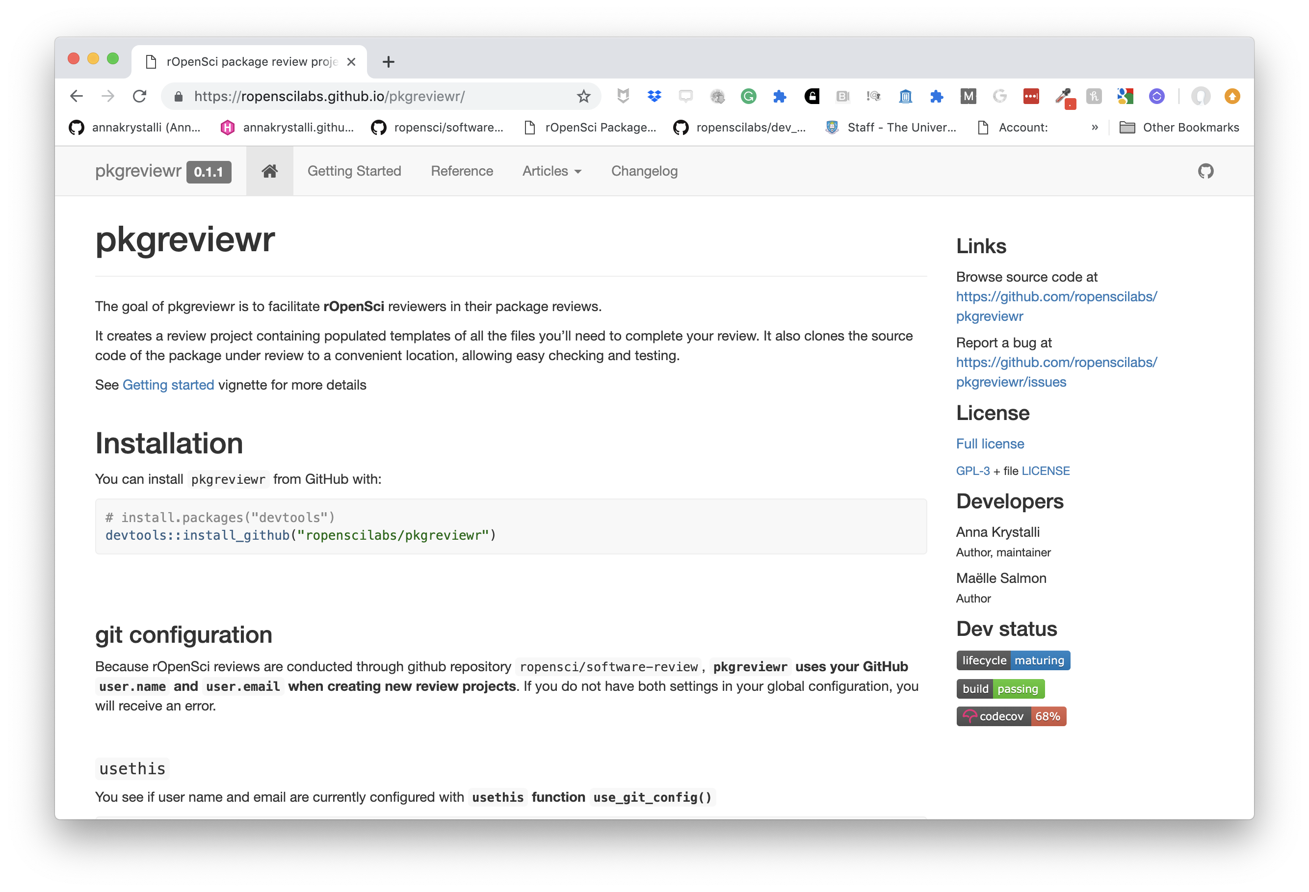
pkgdown
For buidling package documentation
- Can use it to document any functional code you produce and demonstrate it’s us ethrough vignettes
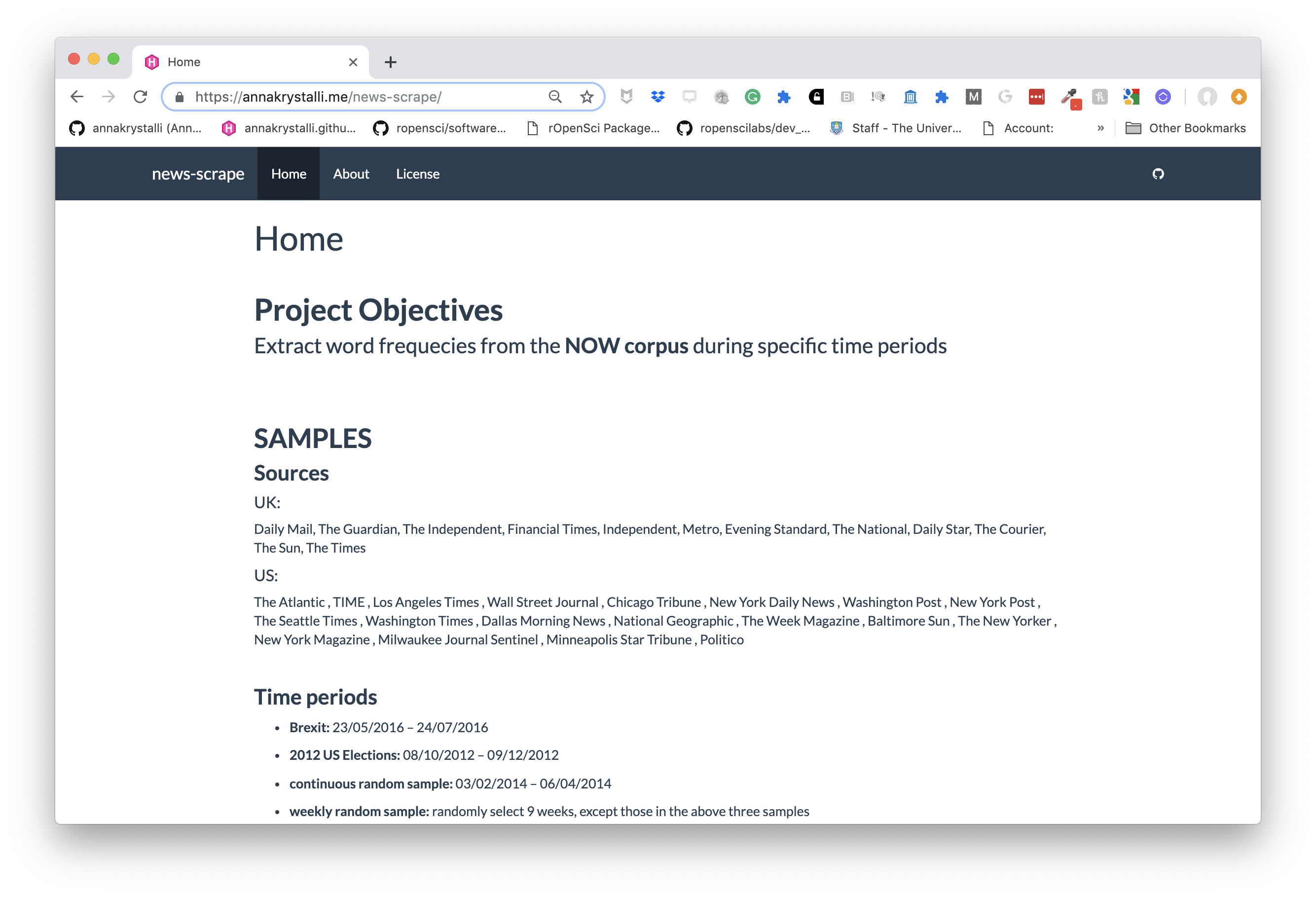
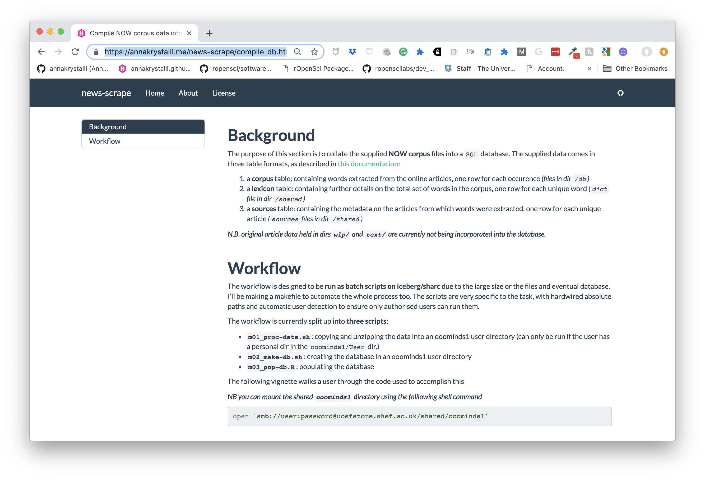
workflowr pkg
Build analyses websites and organise your project
The workflowr R package makes it easier for researchers to organize their projects and share their results with colleagues.
 ] —
] —
blogdown
For creating and mantaining blogs.
Check out https://awesome-blogdown.com/, a curated list of awesome #rstats blogs in blogdown for inspiration!
bookdown
For creating and mantaining online books
Resources
Reproducible Research coursera MOOC
Solutions: My example
R version 3.5.2 (2018-12-20)
Platform: x86_64-apple-darwin15.6.0 (64-bit)
Running under: macOS Mojave 10.14.3

Matrix products: default
BLAS: /Library/Frameworks/R.framework/Versions/3.5/Resources/lib/libRblas.0.dylib
LAPACK: /Library/Frameworks/R.framework/Versions/3.5/Resources/lib/libRlapack.dylib

locale:
[1] en_GB.UTF-8/en_GB.UTF-8/en_GB.UTF-8/C/en_GB.UTF-8/en_GB.UTF-8

attached base packages:
[1] stats     graphics  grDevices utils     datasets  methods   base

other attached packages:
 [1] plotly_4.7.1    gapminder_0.3.0 DT_0.5          knitr_1.22
 [5] forcats_0.4.0   stringr_1.4.0   dplyr_0.8.0.1   purrr_0.3.2
 [9] readr_1.3.1     tidyr_0.8.3     tibble_2.1.1    ggplot2_3.1.0
[13] tidyverse_1.2.1

loaded via a namespace (and not attached):
 [1] Rcpp_1.0.1        here_0.1          lubridate_1.7.4
 [4] lattice_0.20-38   assertthat_0.2.0  rprojroot_1.3-2
 [7] digest_0.6.18     utf8_1.1.4        mime_0.6
[10] R6_2.4.0          cellranger_1.1.0  plyr_1.8.4
[13] backports_1.1.3   evaluate_0.13     httr_1.4.0
[16] highr_0.7         pillar_1.3.1      rlang_0.3.1
[19] lazyeval_0.2.1    readxl_1.3.0      data.table_1.12.0
[22] rstudioapi_0.9.0  whisker_0.3-2     rmarkdown_1.12
[25] labeling_0.3      htmlwidgets_1.3   munsell_0.5.0
[28] shiny_1.2.0       broom_0.5.1       compiler_3.5.2
[31] httpuv_1.5.0      modelr_0.1.3      xfun_0.5
[34] pkgconfig_2.0.2   htmltools_0.3.6   tidyselect_0.2.5
[37] workflowr_1.2.0   emo_0.0.0.9000    viridisLite_0.3.0
[40] fansi_0.4.0       crayon_1.3.4      withr_2.1.2
[43] later_0.8.0       grid_3.5.2        nlme_3.1-137
[46] jsonlite_1.6      xtable_1.8-3      gtable_0.2.0
[49] git2r_0.24.0.9001 magrittr_1.5      formatR_1.5
[52] scales_1.0.0      cli_1.1.0         stringi_1.3.1
[55] fs_1.2.7          promises_1.0.1    skimr_1.0.5
[58] xml2_1.2.0        generics_0.0.2    tools_3.5.2
[61] glue_1.3.1        hms_0.4.2         crosstalk_1.0.0
[64] yaml_2.2.0        colorspace_1.4-0  rvest_0.3.2
[67] haven_2.0.0