20220919_chRNA_IntronRetention
Last updated: 2022-09-22
Checks: 5 2
Knit directory: 20211209_JingxinRNAseq/analysis/
This reproducible R Markdown analysis was created with workflowr (version 1.6.2). The Checks tab describes the reproducibility checks that were applied when the results were created. The Past versions tab lists the development history.
The R Markdown file has unstaged changes. To know which version of the R Markdown file created these results, you’ll want to first commit it to the Git repo. If you’re still working on the analysis, you can ignore this warning. When you’re finished, you can run wflow_publish to commit the R Markdown file and build the HTML.
Great job! The global environment was empty. Objects defined in the global environment can affect the analysis in your R Markdown file in unknown ways. For reproduciblity it’s best to always run the code in an empty environment.
The command set.seed(19900924) was run prior to running the code in the R Markdown file. Setting a seed ensures that any results that rely on randomness, e.g. subsampling or permutations, are reproducible.
Great job! Recording the operating system, R version, and package versions is critical for reproducibility.
Nice! There were no cached chunks for this analysis, so you can be confident that you successfully produced the results during this run.
Using absolute paths to the files within your workflowr project makes it difficult for you and others to run your code on a different machine. Change the absolute path(s) below to the suggested relative path(s) to make your code more reproducible.
| absolute | relative |
|---|---|
| /project2/yangili1/bjf79/20211209_JingxinRNAseq/code/bigwigs/unstranded/(.+?).bw | ../code/bigwigs/unstranded/(.+?).bw |
Great! You are using Git for version control. Tracking code development and connecting the code version to the results is critical for reproducibility.
The results in this page were generated with repository version 7144e91. See the Past versions tab to see a history of the changes made to the R Markdown and HTML files.
Note that you need to be careful to ensure that all relevant files for the analysis have been committed to Git prior to generating the results (you can use wflow_publish or wflow_git_commit). workflowr only checks the R Markdown file, but you know if there are other scripts or data files that it depends on. Below is the status of the Git repository when the results were generated:
Ignored files:
    Ignored:    .DS_Store
    Ignored:    .Rhistory
    Ignored:    .Rproj.user/
    Ignored:    ._.DS_Store
    Ignored:    analysis/.RData
    Ignored:    analysis/.Rhistory
    Ignored:    analysis/20220707_TitrationSeries_DE_testing.nb.html
    Ignored:    code/%
    Ignored:    code/.DS_Store
    Ignored:    code/._.DS_Store
    Ignored:    code/._DOCK7.pdf
    Ignored:    code/._DOCK7_DMSO1.pdf
    Ignored:    code/._DOCK7_SM2_1.pdf
    Ignored:    code/._FKTN_DMSO_1.pdf
    Ignored:    code/._FKTN_SM2_1.pdf
    Ignored:    code/._MAPT.pdf
    Ignored:    code/._PKD1_DMSO_1.pdf
    Ignored:    code/._PKD1_SM2_1.pdf
    Ignored:    code/.snakemake/
    Ignored:    code/1KG_HighCoverageCalls.samplelist.txt
    Ignored:    code/5ssSeqs.tab
    Ignored:    code/Alignments/
    Ignored:    code/ChemCLIP/
    Ignored:    code/ClinVar/
    Ignored:    code/DE_testing/
    Ignored:    code/DE_tests.mat.counts.gz
    Ignored:    code/DE_tests.txt.gz
    Ignored:    code/DoseResponseData/
    Ignored:    code/Fastq/
    Ignored:    code/FastqFastp/
    Ignored:    code/FragLenths/
    Ignored:    code/Meme/
    Ignored:    code/Multiqc/
    Ignored:    code/OMIM/
    Ignored:    code/OldBigWigs/
    Ignored:    code/QC/
    Ignored:    code/Session.vim
    Ignored:    code/SplicingAnalysis/
    Ignored:    code/TracksSession
    Ignored:    code/bigwigs/
    Ignored:    code/featureCounts/
    Ignored:    code/geena/
    Ignored:    code/igv_session.template.xml
    Ignored:    code/igv_session.xml
    Ignored:    code/log
    Ignored:    code/logs/
    Ignored:    code/rules/.RNASeqProcessing.smk.swp
    Ignored:    code/scratch/
    Ignored:    code/test.txt.gz
    Ignored:    code/testPlottingWithMyScript.ForJingxin.sh
    Ignored:    code/testPlottingWithMyScript.ForJingxin2.sh
    Ignored:    code/testPlottingWithMyScript.ForJingxin3.sh
    Ignored:    code/testPlottingWithMyScript.ForJingxin4.sh
    Ignored:    code/testPlottingWithMyScript.sh
    Ignored:    data/._Hijikata_TableS1_41598_2017_8902_MOESM2_ESM.xls
    Ignored:    data/._Hijikata_TableS2_41598_2017_8902_MOESM3_ESM.xls
    Ignored:    output/._PioritizedIntronTargets.pdf

Unstaged changes:
    Modified:   analysis/20220919_chRNA_IntronRetention.Rmd
    Modified:   code/scripts/GenometracksByGenotype
Note that any generated files, e.g. HTML, png, CSS, etc., are not included in this status report because it is ok for generated content to have uncommitted changes.
These are the previous versions of the repository in which changes were made to the R Markdown (analysis/20220919_chRNA_IntronRetention.Rmd) and HTML (docs/20220919_chRNA_IntronRetention.html) files. If you’ve configured a remote Git repository (see ?wflow_git_remote), click on the hyperlinks in the table below to view the files as they were in that past version.
| File | Version | Author | Date | Message |
|---|---|---|---|---|
| Rmd | 7144e91 | Benjmain Fair | 2022-09-21 | added chRNA notebook |
| html | 7144e91 | Benjmain Fair | 2022-09-21 | added chRNA notebook |
Intro
I have quantified intron retention with splice-q package for each sample. I want to investigate the hypothesis that some of the introns affected by small molecules have unique signatures as measured by intron retention or splicing in chRNA dataset. In particular, from looking at the HTT locus below, I notice a few things:
- The drug-induced exon is in a host-intron with a bit more intron retention compared to the surrounding introns in untreated (DMSO) samples. Perhaps introns with slower splicing are a bit predisposed to new drug-induced splicing.
- The drug induced exon is spliced-in at a higher rate (relative to the skipping event) in the chRNA, presumably since NMD quickly degrades the exon-included isoform post-transcriptionally.
- The intron upstream of the drug-induced exon seems to be spliced more efficiently in treated samples, relative to the downstream intron which actually contains the target 5’ GA|GT splice site (black line in screenshot) that interacts with the small molecule. This is reminiscent of early exon definition experiments wherein strengthening a downstream 5’ss enhances splicing of the upstream intron.
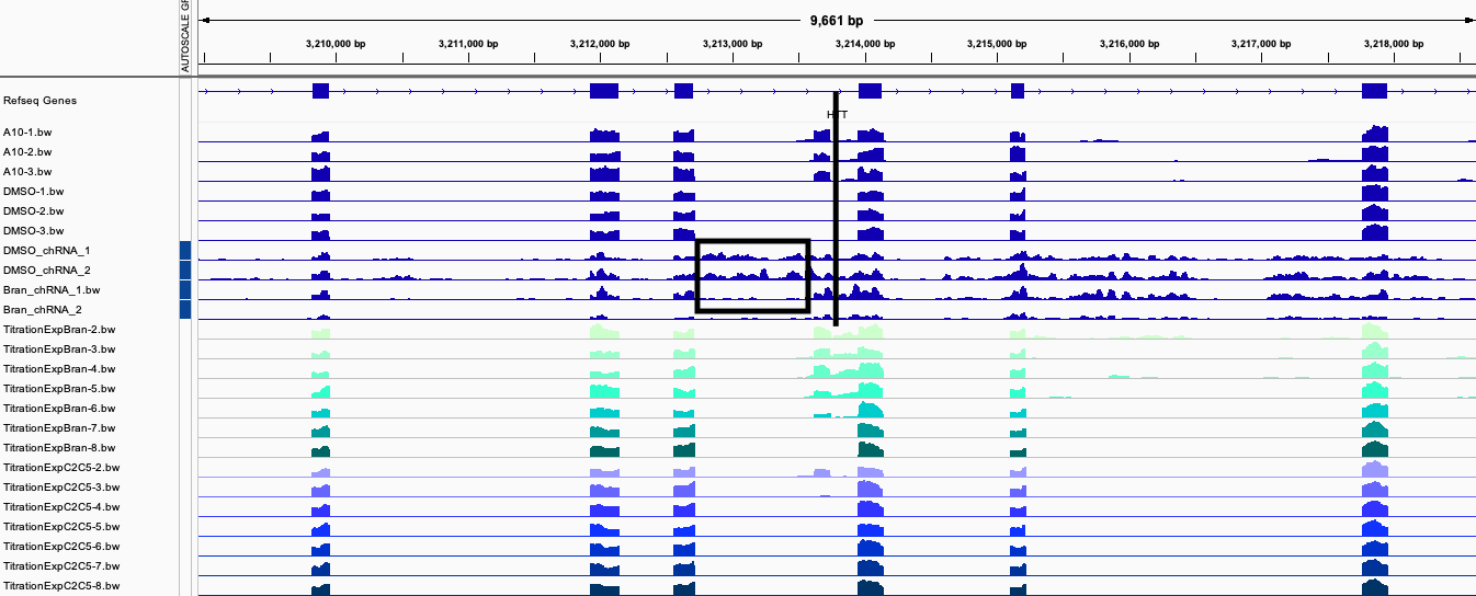
IGVScreenshot
HTT
In this notebook, I will explore whether these observations are representative of drug-induced exons genomewide. First, read in the data…
library(tidyverse)
library(gplots)

#Read in sample metadata
sample.list <- read_tsv("../code/bigwigs/BigwigList.tsv",
                        col_names = c("SampleName", "bigwig", "group", "strand")) %>%
  filter(strand==".") %>%
  mutate(old.sample.name = str_replace(bigwig, "/project2/yangili1/bjf79/20211209_JingxinRNAseq/code/bigwigs/unstranded/(.+?).bw", "\\1")) %>%
  separate(SampleName, into=c("treatment", "dose.nM", "cell.type", "libType", "rep"), convert=T, remove=F, sep="_") %>%
  left_join(
    read_tsv("../code/bigwigs/BigwigList.groups.tsv", col_names = c("group", "color", "bed", "supergroup")),
    by="group"
  )

SampleNameConversionKey <- sample.list %>%
  dplyr::select(SampleName, old.sample.name) %>%
  deframe()

GA.GT.Introns <- read_tsv("../output/EC50Estimtes.FromPSI.txt.gz")

read.SpliceQ.Table <- function(fn){
  read_tsv(fn) %>%
  rename_at(vars(-Intron), ~str_replace(.x, ".+?Merged/(.+?)\\.txt\\.gz", "\\1")) %>%
  rename(!!!SampleNameConversionKey) %>%
  separate(Intron, into=c("Chrom", "start", "stop", "strand"), convert=T, sep="_") %>%
  mutate(stop = stop+1) %>%
  mutate(Chrom=paste0("chr", Chrom)) %>%
  dplyr::select(Chrom:strand, everything())
}

SpliceQ.IER <- read.SpliceQ.Table("../code/SplicingAnalysis/SpliceQ/MergedTable.IER.txt.gz")
SpliceQ.SE <- read.SpliceQ.Table("../code/SplicingAnalysis/SpliceQ/MergedTable.SE.txt.gz")


all.samples.PSI <- read_tsv("../code/SplicingAnalysis/leafcutter_all_samples/PSI.table.bed.gz")

all.samples.5ss <- read_tsv("../code/SplicingAnalysis/FullSpliceSiteAnnotations/JuncfilesMerged.annotated.basic.bed.5ss.tab.gz", col_names = c("intron", "seq", "score")) %>%
  mutate(intron = str_replace(intron, "^(.+?)::.+$", "\\1")) %>%
  separate(intron, into=c("chrom", "start", "stop", "strand"), sep="_", convert=T, remove=F)

all.samples.intron.annotations <- read_tsv("../code/SplicingAnalysis/FullSpliceSiteAnnotations/JuncfilesMerged.annotated.basic.bed.gz")
effect sizes in chRNA versus polyA
Let’s check the first hypothesis… that chRNA will generally show larger effect sizes between ratio of included versus skipped reads.
GA.GT.Introns.DrugInducedCassetteExons <- GA.GT.Introns %>%
  filter(!is.na(Steepness)) %>%
  filter(UpperLimit > LowerLimit) %>%
  filter(!is.na(UpstreamSpliceAcceptor)) %>%
  dplyr::rename(strand=strand.y)


chRNA.Comparison.Samples <- sample.list %>%
  filter(cell.type=="LCL") %>%
  group_by(dose.nM, treatment) %>%
  filter(any(libType=="chRNA"))


IntronsToQuantifyInDrugInducedCassetteExons <- all.samples.PSI %>%
  filter(gid %in% GA.GT.Introns$gid) %>%
  mutate(SpliceAcceptor = case_when(
    strand == "+" ~ paste(`#Chrom`, end, strand, sep="."),
    strand == "-" ~ paste(`#Chrom`, start-2, strand, sep=".")
  )) %>%
  select(1:6, SpliceAcceptor, contains("LCL")) %>%
  gather(key="Sample", value="PSI", contains("LCL")) %>%
  group_by(junc, gid, strand, SpliceAcceptor) %>%
  drop_na() %>%
  summarise(mean=mean(PSI, na.rm = F)) %>%
  group_by(SpliceAcceptor) %>%
  filter(mean == max(mean)) %>%
  ungroup() %>%
  dplyr::select(UpstreamJunc = junc, SpliceAcceptor) %>%
  inner_join(GA.GT.Introns.DrugInducedCassetteExons, by=c("SpliceAcceptor"="UpstreamSpliceAcceptor")) %>%
  rename(DownstreamJunc = junc) %>%
  mutate(SkippingJunc = case_when(
    strand == "+" ~ str_replace(paste(UpstreamJunc, DownstreamJunc), "^(chr.+?):(.+?):(.+?):(clu.+?) (chr.+?):(.+?):(.+?):clu.+$", "\\1:\\2:\\7:\\4"),
    strand == "-" ~ str_replace(paste(UpstreamJunc, DownstreamJunc), "^(chr.+?):(.+?):(.+?):(clu.+?) (chr.+?):(.+?):(.+?):clu.+$", "\\1:\\6:\\3:\\4")
  )) %>%
  dplyr::select(UpstreamJunc,DownstreamJunc, SkippingJunc ) %>%
  gather(key="IntronType", value="junc") %>%
  distinct(.keep_all = T) %>%
  mutate(gid = str_replace(junc, ".+?:(clu.+$)", "\\1")) %>%
  add_count(gid) %>%
  filter(n==3)

chRNA.Comparison.PSI.Inclusion.tidy <- IntronsToQuantifyInDrugInducedCassetteExons %>%
  dplyr::select(-n, -gid) %>%
  inner_join(
    all.samples.PSI %>%
      select(1:6, chRNA.Comparison.Samples$SampleName),
    by="junc"
  ) %>%
  gather("Sample", "PSI", contains("LCL")) %>%
  pivot_wider(names_from = "IntronType", values_from="PSI", id_cols=c("gid", "Sample")) %>%
  unnest() %>%
  mutate(InclusionPSI=UpstreamJunc+DownstreamJunc) %>%
  separate(Sample, into=c("treatment", "dose.nM", "cell.type", "libType", "rep"), sep="_", convert=T) %>%
  group_by("treatment", "dose.nM") %>%
  filter(any(libType == "chRNA")) %>%
  ungroup() %>%
  group_by(gid, treatment, dose.nM, cell.type, libType) %>%
  summarise_at(vars(UpstreamJunc:InclusionPSI), mean, na.rm=T) %>%
  mutate(TreatedOrControl = if_else(treatment=="DMSO", "Control", "Treatment")) %>%
  ungroup()


inner_join(
    chRNA.Comparison.PSI.Inclusion.tidy %>%
      filter(TreatedOrControl == "Treatment") %>%
      dplyr::select(-TreatedOrControl),
    chRNA.Comparison.PSI.Inclusion.tidy %>%
      filter(TreatedOrControl == "Control") %>%
      dplyr::select(-TreatedOrControl, -treatment, -dose.nM),
    by=c("gid", "cell.type", "libType"),
    suffix=c(".treatment", ".control")) %>%
  inner_join(
  sample.list %>%
    filter(cell.type=="LCL") %>%
    distinct(treatment, dose.nM, color)) %>%
ggplot(aes(x=InclusionPSI.treatment-InclusionPSI.control, color=color)) +
  stat_ecdf(aes(linetype=libType)) +
  scale_color_identity() +
  facet_wrap(~treatment) +
  theme_bw() +
  labs(title="Comparing DeltaPSI in drug-induced exons (treatment - DMSO)", y="ecdf",
       caption="Darker color is higher dose\nPSI_treatment-PSIcontrol")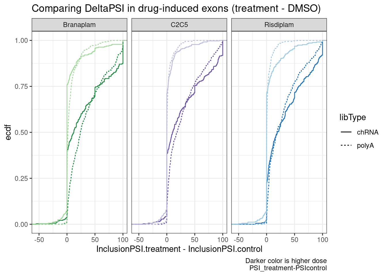
| Version | Author | Date |
|---|---|---|
| 7144e91 | Benjmain Fair | 2022-09-21 |
inner_join(
    chRNA.Comparison.PSI.Inclusion.tidy %>%
      filter(TreatedOrControl == "Treatment") %>%
      dplyr::select(-TreatedOrControl),
    chRNA.Comparison.PSI.Inclusion.tidy %>%
      filter(TreatedOrControl == "Control") %>%
      dplyr::select(-TreatedOrControl, -treatment, -dose.nM),
    by=c("gid", "cell.type", "libType"),
    suffix=c(".treatment", ".control")) %>%
  inner_join(
  sample.list %>%
    filter(cell.type=="LCL") %>%
    distinct(treatment, dose.nM, color)) %>%
ggplot(aes(x=InclusionPSI.treatment/InclusionPSI.control, color=color)) +
  stat_ecdf(aes(linetype=libType)) +
  scale_color_identity() +
  scale_x_continuous(trans="log2") +
  facet_wrap(~treatment) +
  theme_bw() +
  labs(title="Comparing DeltaPSI in drug-induced exons (treatment / DMSO)", y="ecdf",
       caption="Darker color is higher dose\nPSI_treatment/PSIcontrol")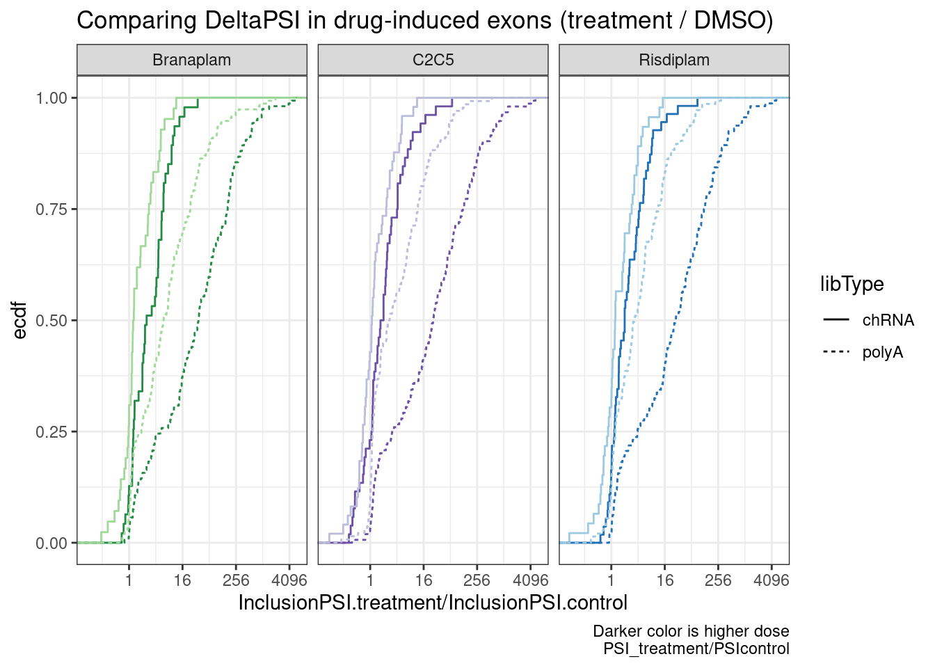
| Version | Author | Date |
|---|---|---|
| 7144e91 | Benjmain Fair | 2022-09-21 |
Ok, so while we can see these exons have a generally positive deltaPSI (as expected, by design of how i filtered the data), and the deltaPSI is more positive at higher dose, it doesn’t seem that the deltaPSI is any bigger in chRNA. And how you choose to the process the data makes all the difference (Difference in PSI, versus Ratio).
inner_join(
    chRNA.Comparison.PSI.Inclusion.tidy %>%
      filter(TreatedOrControl == "Treatment") %>%
      dplyr::select(-TreatedOrControl),
    chRNA.Comparison.PSI.Inclusion.tidy %>%
      filter(TreatedOrControl == "Control") %>%
      dplyr::select(-TreatedOrControl, -treatment, -dose.nM),
    by=c("gid", "cell.type", "libType"),
    suffix=c(".treatment", ".control")) %>%
  inner_join(
  sample.list %>%
    filter(cell.type=="LCL") %>%
    distinct(treatment, dose.nM, color)) %>%
ggplot(aes(x=(InclusionPSI.treatment/SkippingJunc.treatment)/(InclusionPSI.control/SkippingJunc.control), color=color)) +
  stat_ecdf(aes(linetype=libType)) +
  scale_color_identity() +
  scale_x_continuous(trans="log2") +
  facet_wrap(~treatment) +
  theme_bw() +
  labs(title="Comparing DeltaPSI in drug-induced exons (treatment / DMSO)", y="ecdf",
       caption="Darker color is higher dose\nPSI_treatment/PSIcontrol")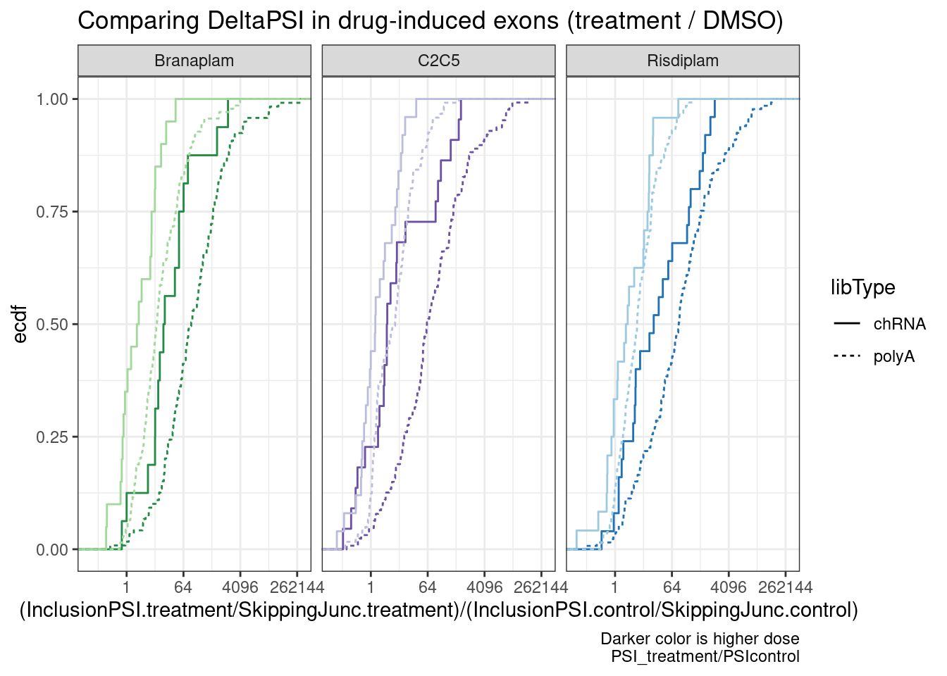
| Version | Author | Date |
|---|---|---|
| 7144e91 | Benjmain Fair | 2022-09-21 |
AddPsuedocount <- function(x){
  return(x+0.01)
}

dat.to.plot <- inner_join(
    chRNA.Comparison.PSI.Inclusion.tidy %>%
      filter(TreatedOrControl == "Treatment") %>%
      dplyr::select(-TreatedOrControl),
    chRNA.Comparison.PSI.Inclusion.tidy %>%
      filter(TreatedOrControl == "Control") %>%
      dplyr::select(-TreatedOrControl, -treatment, -dose.nM),
    by=c("gid", "cell.type", "libType"),
    suffix=c(".treatment", ".control")) %>%
  inner_join(
  sample.list %>%
    filter(cell.type=="LCL") %>%
    distinct(treatment, dose.nM, color)) %>%
  #Add pseudocount to PSI
  mutate_at(vars(UpstreamJunc.treatment:InclusionPSI.control), AddPsuedocount) %>%
  mutate(SkippingToInclusionRatio = (InclusionPSI.treatment/SkippingJunc.treatment)/(InclusionPSI.control/SkippingJunc.control)) %>%
  dplyr::select(-(UpstreamJunc.treatment:InclusionPSI.control)) %>%
  pivot_wider(names_from="libType", values_from="SkippingToInclusionRatio")

ggplot(dat.to.plot, aes(x=(chRNA/polyA), color=color)) +
  geom_vline(xintercept=1) +
  stat_ecdf() +
  scale_color_identity() +
  scale_x_continuous(trans="log10") +
  facet_wrap(~treatment) +
  theme_bw() +
  labs(title="effect sizes don't appear stronger in chRNA", y="ecdf",
       x="DrugInducedSkippingRatio_chRNA/DrugInducedSkippingRatio_polyA",
       caption="DrugInducedSkippingRatio = (PSI_included_treatment/PSI_skip_treatment)/(PSI_included_control/PSI_skip_control)")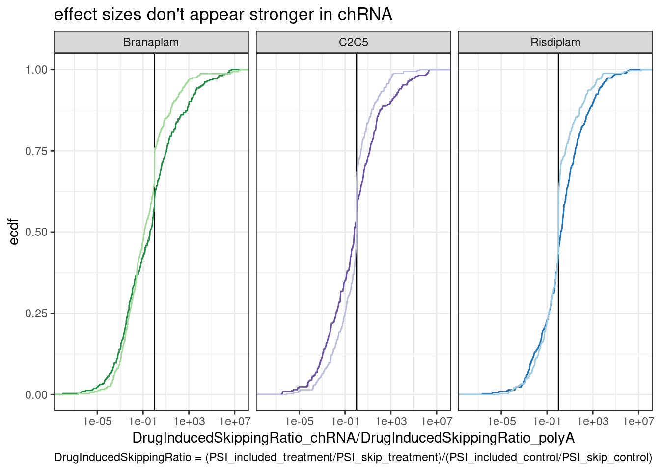
| Version | Author | Date |
|---|---|---|
| 7144e91 | Benjmain Fair | 2022-09-21 |
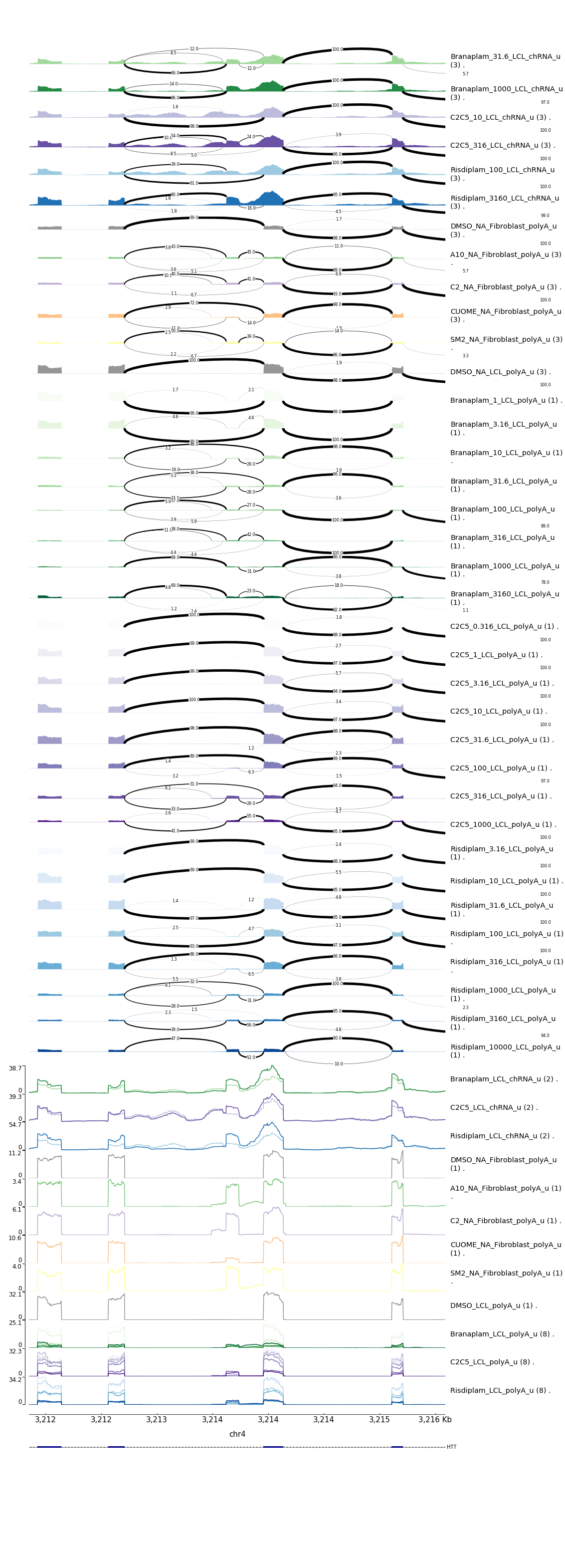
And to verify that I did the analysis reasonably, let’s look at the HTT skipping event, where I know (from manually inspecting the screenshot at the top with the sashimi plots of the raw PSI) that chRNA should have a higher DrugInducedSkipping Ratio in branaplam
GA.GT.Introns.DrugInducedCassetteExons %>%
  filter(gene_names == "HTT")
# A tibble: 1 × 34
junc `#Chrom` start end gid strand seq Donor.score gene_names
<chr> <chr> <dbl> <dbl> <chr> <chr> <chr> <dbl> <chr>
1 chr4:3213736… chr4 3.21e6 3.21e6 chr4… + CAGA… 5.53 HTT
# … with 25 more variables: gene_ids <chr>, SpliceDonor <chr>,
# UpstreamSpliceAcceptor <chr>, IntronType <chr>, Steepness <dbl>,
# LowerLimit <dbl>, UpperLimit <dbl>, ED50_Branaplam <dbl>, ED50_C2C5 <dbl>,
# ED50_Risdiplam <dbl>, spearman.coef.Branaplam <dbl>,
# spearman.coef.C2C5 <dbl>, spearman.coef.Risdiplam <dbl>,
# EC.Ratio.Test.Estimate_Branaplam.C2C5 <dbl>,
# EC.Ratio.Test.Estimate_Branaplam.Risdiplam <dbl>, …dat.to.plot %>%
filter(gid=="chr4_clu_9322_+")# A tibble: 6 × 7
gid treatment dose.nM cell.type color chRNA polyA
<chr> <chr> <dbl> <chr> <chr> <dbl> <dbl>
1 chr4_clu_9322_+ Branaplam 31.6 LCL #A1D99B 63164. 2118.
2 chr4_clu_9322_+ Branaplam 1000 LCL #238B45 86351968. 12502500.
3 chr4_clu_9322_+ C2C5 10 LCL #BCBDDC 164. 0.125
4 chr4_clu_9322_+ C2C5 316 LCL #6A51A3 153728. 2500.
5 chr4_clu_9322_+ Risdiplam 100 LCL #9ECAE1 6395. 96.9
6 chr4_clu_9322_+ Risdiplam 3160 LCL #2171B5 96352968. 78659. …as expected. Overall I don’t think drug-induced exons are actually that more apparent in chRNA. Later I will peruse a large handful of sashimi plots to make verify. Now let’s move on to looking at the natural splicing rate of introns that host the drug-induced exons…
Host intron inclusion of drug-induced introns
First let’s look at the correlation matrix based on IntronExcisionRatio and SpliceEfficiency metrics (see SpliceQ paper) for the GA|GT introns that I previously fit dose-response curves to… Since
GA.GT.Introns.DrugInducedCassetteExons# A tibble: 454 × 34
junc `#Chrom` start end gid strand seq Donor.score gene_names
<chr> <chr> <dbl> <dbl> <chr> <chr> <chr> <dbl> <chr>
1 chr1:120396… chr1 1.20e6 1.20e6 chr1… - AGGA… 4.21 TNFRSF18
2 chr1:836597… chr1 8.37e6 8.40e6 chr1… - AAGA… 5.57 RERE
3 chr1:971413… chr1 9.71e6 9.72e6 chr1… + AGGA… 4.27 PIK3CD
4 chr1:119818… chr1 1.20e7 1.20e7 chr1… + ATGA… 3.40 MFN2
5 chr1:120660… chr1 1.21e7 1.21e7 chr1… + GAGA… 1.60 <NA>
6 chr1:154268… chr1 1.54e7 1.54e7 chr1… + CAGA… 4.22 EFHD2
7 chr1:238632… chr1 2.39e7 2.39e7 chr1… - AGGA… 3.08 FUCA1
8 chr1:238756… chr1 2.39e7 2.39e7 chr1… - AAGA… 4.84 CNR2
9 chr1:281725… chr1 2.82e7 2.82e7 chr1… - AGGA… 5.37 <NA>
10 chr1:292069… chr1 2.92e7 2.92e7 chr1… - CAGA… 4.60 MECR
# … with 444 more rows, and 25 more variables: gene_ids <chr>,
# SpliceDonor <chr>, UpstreamSpliceAcceptor <chr>, IntronType <chr>,
# Steepness <dbl>, LowerLimit <dbl>, UpperLimit <dbl>, ED50_Branaplam <dbl>,
# ED50_C2C5 <dbl>, ED50_Risdiplam <dbl>, spearman.coef.Branaplam <dbl>,
# spearman.coef.C2C5 <dbl>, spearman.coef.Risdiplam <dbl>,
# EC.Ratio.Test.Estimate_Branaplam.C2C5 <dbl>,
# EC.Ratio.Test.Estimate_Branaplam.Risdiplam <dbl>, …chRNA.Comparison.PSI.Inclusion.tidy# A tibble: 5,474 × 10
gid treatment dose.nM cell.type libType UpstreamJunc DownstreamJunc
<chr> <chr> <dbl> <chr> <chr> <dbl> <dbl>
1 chr10_clu_19… Branaplam 31.6 LCL chRNA 0 0
2 chr10_clu_19… Branaplam 31.6 LCL polyA 0 3.5
3 chr10_clu_19… Branaplam 1000 LCL chRNA 0 0
4 chr10_clu_19… Branaplam 1000 LCL polyA 16 7.8
5 chr10_clu_19… C2C5 10 LCL chRNA 25 0
6 chr10_clu_19… C2C5 10 LCL polyA 4.7 0
7 chr10_clu_19… C2C5 316 LCL chRNA 22 0
8 chr10_clu_19… C2C5 316 LCL polyA 7.9 13
9 chr10_clu_19… DMSO NA LCL chRNA 0 0
10 chr10_clu_19… DMSO NA LCL polyA 0 0
# … with 5,464 more rows, and 3 more variables: SkippingJunc <dbl>,
# InclusionPSI <dbl>, TreatedOrControl <chr>HostIntronsToQuantifyInDrugInducedCassetteExons <- IntronsToQuantifyInDrugInducedCassetteExons %>%
pivot_wider(names_from="IntronType", values_from="junc") %>%
separate(SkippingJunc, into=c("Chrom", "start","stop","cluster"), sep=":", convert=T) %>%
mutate(strand = str_extract(cluster, "[+-]"))
SpliceQ.IER %>%
dplyr::select(1:4, matches("DMSO_NA_LCL_chRNA_.+")) %>%
gather("Sample", "IER", contains("DMSO")) %>%
group_by(Chrom, start, stop, strand) %>%
summarise(IER.mean=mean(IER)) %>%
inner_join(all.samples.intron.annotations, by=c("Chrom"="chrom", "start", "stop"="end", "strand")) %>%
left_join(HostIntronsToQuantifyInDrugInducedCassetteExons) %>%
group_by(gene_ids) %>%
filter(any(!is.na(UpstreamJunc))) %>%
ungroup() %>%
ggplot(aes(x=IER.mean)) +
stat_ecdf() +
geom_vline(
data = . %>% filter(!is.na(UpstreamJunc)),
aes(xintercept=IER.mean)
) +
facet_wrap(~gene_names) +
theme_bw() +
labs(y="ecdf", x="IntronExcisionRatio", title="IER distribution of host introns, compared to other introns in host gene")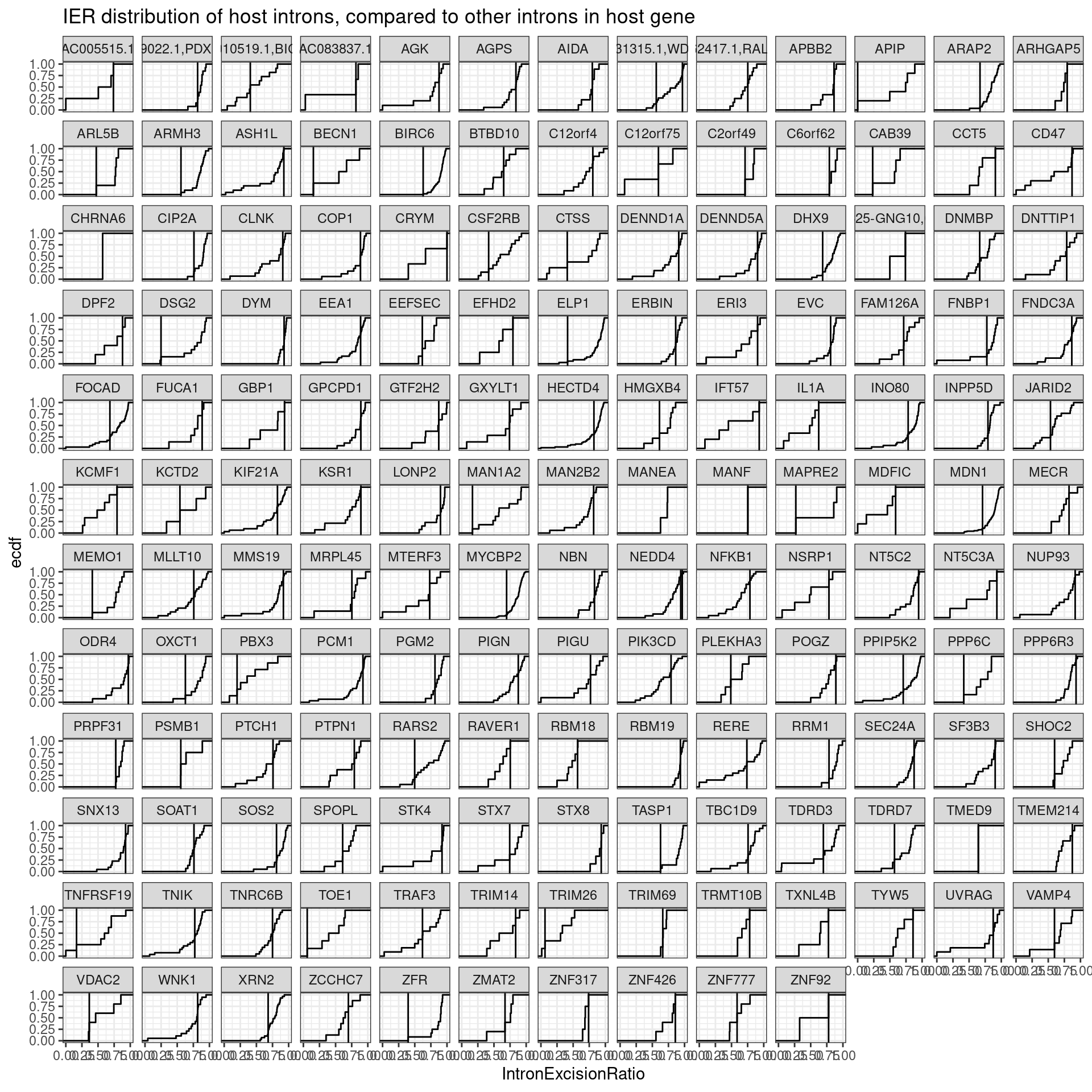
| Version | Author | Date |
|---|---|---|
| 7144e91 | Benjmain Fair | 2022-09-21 |
Hmmm, It’s not obvious if there is a trend… I was hypothesizing that introns hosting the cassette exon would have have lower intron excision ratios, indicating less efficient splicing. Let’s plot this a few different ways:
SpliceQ.IER %>%
  dplyr::select(1:4, matches("DMSO_NA_LCL_chRNA_.+")) %>%
  gather("Sample", "IER", contains("DMSO")) %>%
  group_by(Chrom, start, stop, strand) %>%
  summarise(IER.mean=mean(IER)) %>%
  inner_join(all.samples.intron.annotations, by=c("Chrom"="chrom", "start", "stop"="end", "strand")) %>%
  left_join(HostIntronsToQuantifyInDrugInducedCassetteExons) %>%
  group_by(gene_ids) %>%
  filter(any(!is.na(UpstreamJunc))) %>%
  ungroup() %>%
  mutate(IsHostIntronOfDrugInducedCassetteExon = if_else(is.na(UpstreamJunc), "Control Intron", "Host Intron")) %>%
  # group_by(gene_names, IsHostIntronOfDrugInducedCassetteExon) %>%
  # sample_n(1) %>%
  ggplot(aes(x=IER.mean, color=IsHostIntronOfDrugInducedCassetteExon)) +
  stat_ecdf() +
  theme_bw() +
  labs(y="ecdf", x="IntronExcisionRatio", caption=str_wrap("Comparing introns hosting the drug-induced cassette exons to all introns within the same set of genes", 50))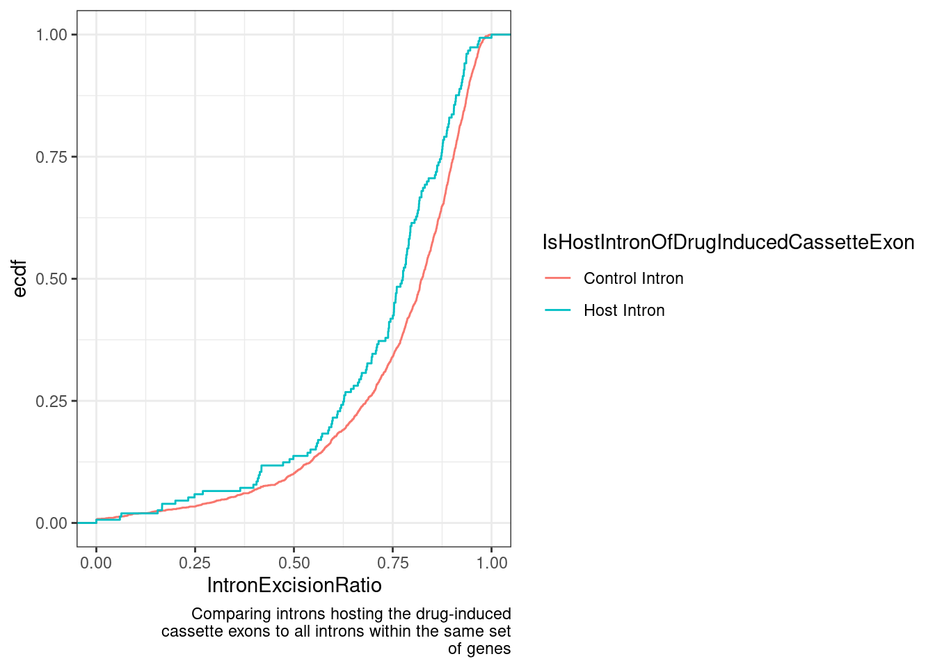
| Version | Author | Date |
|---|---|---|
| 7144e91 | Benjmain Fair | 2022-09-21 |
The intron excision ratio metric is basically the length-normalized intronic coverage, relative to the flanking exons… So if there is a cassette exon that is spliced in at an appreciable rate in DMSO samples, that might explain this. The splice efficiency metric, based only on exon-exon junction and exon-intron, intron-exon reads should be less sensitive to this. let’s check that the effect is there too.
SpliceQ.SE %>%
  dplyr::select(1:4, matches("DMSO_NA_LCL_chRNA_.+")) %>%
  gather("Sample", "IER", contains("DMSO")) %>%
  group_by(Chrom, start, stop, strand) %>%
  summarise(IER.mean=mean(IER)) %>%
  inner_join(all.samples.intron.annotations, by=c("Chrom"="chrom", "start", "stop"="end", "strand")) %>%
  left_join(HostIntronsToQuantifyInDrugInducedCassetteExons) %>%
  group_by(gene_ids) %>%
  filter(any(!is.na(UpstreamJunc))) %>%
  ungroup() %>%
  mutate(IsHostIntronOfDrugInducedCassetteExon = if_else(is.na(UpstreamJunc), "Control Intron", "Host Intron")) %>%
  # group_by(gene_names, IsHostIntronOfDrugInducedCassetteExon) %>%
  # sample_n(1) %>%
  ggplot(aes(x=IER.mean, color=IsHostIntronOfDrugInducedCassetteExon)) +
  stat_ecdf() +
  theme_bw() +
  labs(y="ecdf", x="SpicingEfficiency", caption=str_wrap("Comparing introns hosting the drug-induced cassette exons to all introns within the same set of genes", 50))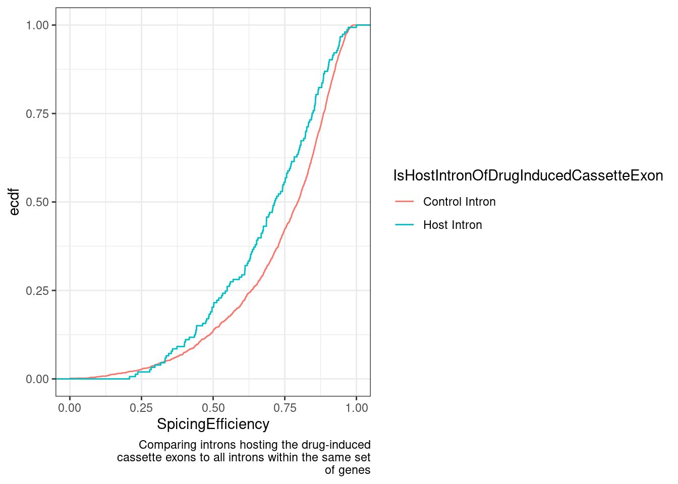
| Version | Author | Date |
|---|---|---|
| 7144e91 | Benjmain Fair | 2022-09-21 |
Hm, here there is some very modest effect, but I will get to doing a more proper test for significance later.
Finally I want to get to the question about whether that exon-definition effect was apparent, wherein the upstream intron has more efficient splicing… I think I’ll do this later, as it requires me to quantify intron retention in unannotated introns, which isn’t in the existing intron retention quantifications that I made using splice-q.
sessionInfo()R version 3.6.1 (2019-07-05)
Platform: x86_64-pc-linux-gnu (64-bit)
Running under: CentOS Linux 7 (Core)
Matrix products: default
BLAS/LAPACK: /software/openblas-0.2.19-el7-x86_64/lib/libopenblas_haswellp-r0.2.19.so
locale:
[1] LC_CTYPE=en_US.UTF-8 LC_NUMERIC=C LC_TIME=C
[4] LC_COLLATE=C LC_MONETARY=C LC_MESSAGES=C
[7] LC_PAPER=C LC_NAME=C LC_ADDRESS=C
[10] LC_TELEPHONE=C LC_MEASUREMENT=C LC_IDENTIFICATION=C
attached base packages:
[1] stats graphics grDevices utils datasets methods base
other attached packages:
[1] gplots_3.0.1.1 forcats_0.4.0 stringr_1.4.0 dplyr_1.0.9
[5] purrr_0.3.4 readr_1.3.1 tidyr_1.2.0 tibble_3.1.7
[9] ggplot2_3.3.6 tidyverse_1.3.0
loaded via a namespace (and not attached):
[1] Rcpp_1.0.5 lubridate_1.7.4 gtools_3.9.2.2 assertthat_0.2.1
[5] rprojroot_2.0.2 digest_0.6.20 utf8_1.1.4 R6_2.4.0
[9] cellranger_1.1.0 backports_1.4.1 reprex_0.3.0 evaluate_0.15
[13] httr_1.4.4 highr_0.9 pillar_1.7.0 rlang_1.0.5
[17] readxl_1.3.1 gdata_2.18.0 rstudioapi_0.14 whisker_0.3-2
[21] rmarkdown_1.13 labeling_0.3 munsell_0.5.0 broom_1.0.0
[25] compiler_3.6.1 httpuv_1.5.1 modelr_0.1.8 xfun_0.31
[29] pkgconfig_2.0.2 htmltools_0.5.3 tidyselect_1.1.2 workflowr_1.6.2
[33] fansi_0.4.0 crayon_1.3.4 dbplyr_1.4.2 withr_2.5.0
[37] later_0.8.0 bitops_1.0-6 grid_3.6.1 jsonlite_1.6
[41] gtable_0.3.0 lifecycle_1.0.1 DBI_1.1.0 git2r_0.26.1
[45] magrittr_1.5 scales_1.1.0 KernSmooth_2.23-15 cli_3.3.0
[49] stringi_1.4.3 farver_2.1.0 fs_1.5.2 promises_1.0.1
[53] xml2_1.3.2 ellipsis_0.3.2 generics_0.1.3 vctrs_0.4.1
[57] tools_3.6.1 glue_1.6.2 hms_0.5.3 fastmap_1.1.0
[61] yaml_2.2.0 colorspace_1.4-1 caTools_1.17.1.2 rvest_0.3.5
[65] knitr_1.39 haven_2.3.1