Plot ARCHS4 gene expression data
2024-08-04
Last updated: 2024-08-04
Checks: 7 0
Knit directory: muse/
This reproducible R Markdown analysis was created with workflowr (version 1.7.1). The Checks tab describes the reproducibility checks that were applied when the results were created. The Past versions tab lists the development history.
Great! Since the R Markdown file has been committed to the Git repository, you know the exact version of the code that produced these results.
Great job! The global environment was empty. Objects defined in the global environment can affect the analysis in your R Markdown file in unknown ways. For reproduciblity it’s best to always run the code in an empty environment.
The command set.seed(20200712) was run prior to running
the code in the R Markdown file. Setting a seed ensures that any results
that rely on randomness, e.g. subsampling or permutations, are
reproducible.
Great job! Recording the operating system, R version, and package versions is critical for reproducibility.
Nice! There were no cached chunks for this analysis, so you can be confident that you successfully produced the results during this run.
Great job! Using relative paths to the files within your workflowr project makes it easier to run your code on other machines.
Great! You are using Git for version control. Tracking code development and connecting the code version to the results is critical for reproducibility.
The results in this page were generated with repository version 0b486eb. See the Past versions tab to see a history of the changes made to the R Markdown and HTML files.
Note that you need to be careful to ensure that all relevant files for
the analysis have been committed to Git prior to generating the results
(you can use wflow_publish or
wflow_git_commit). workflowr only checks the R Markdown
file, but you know if there are other scripts or data files that it
depends on. Below is the status of the Git repository when the results
were generated:
Ignored files:
    Ignored:    .Rhistory
    Ignored:    .Rproj.user/
    Ignored:    r_packages_4.3.3/
    Ignored:    r_packages_4.4.0/
Note that any generated files, e.g. HTML, png, CSS, etc., are not included in this status report because it is ok for generated content to have uncommitted changes.
These are the previous versions of the repository in which changes were
made to the R Markdown (analysis/gene_heatmap.Rmd) and HTML
(docs/gene_heatmap.html) files. If you’ve configured a
remote Git repository (see ?wflow_git_remote), click on the
hyperlinks in the table below to view the files as they were in that
past version.
| File | Version | Author | Date | Message |
|---|---|---|---|---|
| Rmd | 0b486eb | Dave Tang | 2024-08-04 | Fix headers |
| html | 14838f9 | Dave Tang | 2024-08-04 | Build site. |
| Rmd | aeb4c85 | Dave Tang | 2024-08-04 | Aesthetics |
| html | 9e8e5a9 | Dave Tang | 2024-08-04 | Build site. |
| Rmd | f34237f | Dave Tang | 2024-08-04 | Manually calculate the correlation |
| html | 3030a3c | Dave Tang | 2024-08-03 | Build site. |
| Rmd | ee40673 | Dave Tang | 2024-08-03 | Top 100 most correlated |
| html | 42c3d39 | Dave Tang | 2024-08-03 | Build site. |
| Rmd | b5aa7d6 | Dave Tang | 2024-08-03 | Plot TNF expression as a boxplot |
| html | df00969 | Dave Tang | 2023-07-14 | Build site. |
| Rmd | 7188c55 | Dave Tang | 2023-07-14 | pheatmap resolution |
| html | e2d73eb | Dave Tang | 2023-07-14 | Build site. |
| Rmd | 3a5ec3f | Dave Tang | 2023-07-14 | Interactive heatmap |
| html | 7fa8b41 | Dave Tang | 2023-07-13 | Build site. |
| Rmd | 922aa56 | Dave Tang | 2023-07-13 | ARCHS4 heatmap |
ARCHS4
Use gget and the archs4 subtool to find the most correlated genes to a gene of interest or find the gene’s tissue expression atlas using ARCHS4.
Install using pip:
pip install --upgrade ggetUsage.
gget archs4 -husage: gget archs4 [-h] [-e] [-w {correlation,tissue}] [-gc GENE_COUNT] [-s {human,mouse}] [-csv] [-o OUT] [-q] [-g GENE_DEPRECATED] [-j] gene
Find the most correlated genes or the tissue expression atlas of a gene using data from the human and mouse RNA-seq database ARCHS4 (https://maayanlab.cloud/archs4/).
positional arguments:
gene Gene symbol or Ensembl gene ID of gene of interest, e.g. 'STAT4'.
options:
-h, --help show this help message and exit
-e, --ensembl Add this flag if gene is given as an Ensembl gene ID. (default: False)
-w {correlation,tissue}, --which {correlation,tissue}
'correlation' (default) or 'tissue'.
- 'correlation' returns a gene correlation table that contains the 100 most correlated genes to the gene of interest. The Pearson correlation is calculated over all samples and tissues in ARCHS4.
- 'tissue' returns a tissue expression atlas calculated from human or mouse samples (as defined by 'species') in ARCHS4. (default: correlation)
-gc GENE_COUNT, --gene_count GENE_COUNT
Number of correlated genes to return (default: 100).
(Only for gene correlation.) (default: 100)
-s {human,mouse}, --species {human,mouse}
'human' (default) or 'mouse'. (Only for tissue expression atlas.) (default: human)
-csv, --csv Returns results in csv format instead of json. (default: True)
-o OUT, --out OUT Path to the csv file the results will be saved in, e.g. path/to/directory/results.csv.
Default: Standard out.
-q, --quiet Does not print progress information. (default: True)
-g GENE_DEPRECATED, --gene GENE_DEPRECATED
DEPRECATED - use positional argument instead. Gene symbol or Ensembl gene ID of gene of interest (str), e.g. 'STAT4'.
-j, --json DEPRECATED - json is now the default output format (convert to csv using flag [--csv]). (default: False)Get tissue expression for TNF and CCL4 in CSV.
gget archs4 --which tissue --csv --out TNF_tissue.csv TNF
gget archs4 --which tissue --csv --out CCL4_tissue.csv CCL4
Get the 100 most correlated genes to TNF from ARCHS4.
gget archs4 --which correlation --csv --out TNF_correlation.csv TNFTissue expression
Load data and split the ID into multiple columns.
read_tissue <- function(fn){
  readr::read_csv(file = fn, show_col_types = FALSE) |>
    tidyr::separate(col = id, sep = "\\.", into = c("junk", "system", "organ", "tissue")) |>
    dplyr::mutate(tissue = stringr::str_to_title(tissue)) |>
    dplyr::arrange(system) |>
    dplyr::mutate(tissue = factor(tissue, levels = tissue)) -> tnf_exp
}

tnf_exp <- read_tissue("data/archs4/TNF_tissue.csv")
ccl4_exp <- read_tissue("data/archs4/CCL4_tissue.csv")
head(tnf_exp)
# A tibble: 6 × 9
junk system organ tissue min q1 median q3 max
<chr> <chr> <chr> <fct> <dbl> <dbl> <dbl> <dbl> <dbl>
1 System Cardiovascular System Heart Valve 0.114 1.21 3.23 4.30 5.16
2 System Cardiovascular System Heart Ventr… 0.114 2.16 2.78 3.39 4.31
3 System Cardiovascular System Heart Atrium 0.114 0.114 1.21 2.78 3.35
4 System Cardiovascular System Heart Heart 0.114 0.114 0.114 2.42 8.60
5 System Connective Tissue Adipose ti… Adipo… 0.114 0.114 2.42 3.29 4.84
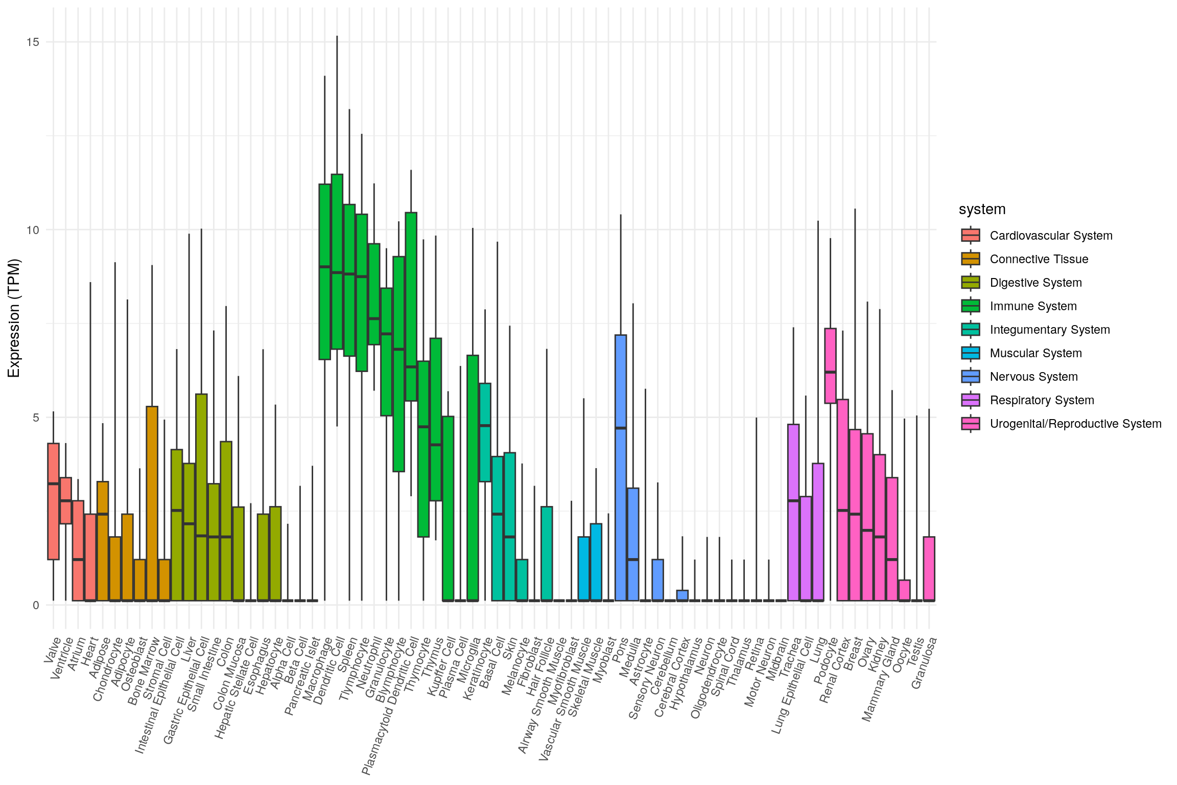
6 System Connective Tissue Bone marrow Chond… 0.114 0.114 0.114 1.81 9.13Plot tissue expression as box plots.
library(ggplot2)
ggplot(
  tnf_exp,
  aes(
    x = tissue,
    ymin = min,
    lower = q1,
    middle = median,
    upper = q3,
    ymax = max,
    fill = system
  )
) +
  geom_boxplot(stat = 'identity') +
  theme_minimal() +
  theme(
    legend.position = 'right',
    axis.title.x = element_blank(),
    axis.text.x = element_text(angle = 70, hjust = 1)
  ) +
  labs(y = "Expression (TPM)")
Combine all data
Tissue expression was retrieved for a list of other genes. We will combine their expressions together into one data frame.
lapply(
  list.files("data/archs4/cancer", pattern = ".csv$", full.names = TRUE),
  function(x){
    cbind(gene = sub("\\.\\w+$", "", basename(x)), read.csv(x))
  }
) |>
  do.call("rbind", args = _) -> my_df

# Split `id` column.
do.call("rbind", strsplit(x = my_df$id, split = "\\.")) |>
  as.data.frame() -> id_split

colnames(id_split) <- c('root', 'system', 'organ', 'tissue')

# Rename tissues.
cap_first <- function(x){
  s <- strsplit(x, "")[[1]][1]
  return(sub(s, toupper(s), x))
}

id_split$tissue <- tolower(id_split$tissue)
id_split$tissue <- sapply(id_split$tissue, cap_first)

my_df <- cbind(my_df, id_split)

# Order `my_df` by system.
my_df <- my_df[order(my_df$gene, my_df$system), ]
my_df$tissue <- factor(my_df$tissue, levels = unique(my_df$tissue))

head(my_df)
gene id min q1
12 CCND1 System.Cardiovascular System.Heart.VALVE 10.62560 11.68490
28 CCND1 System.Cardiovascular System.Heart.HEART 5.87724 10.15820
30 CCND1 System.Cardiovascular System.Heart.VENTRICLE 9.54469 10.37180
36 CCND1 System.Cardiovascular System.Heart.ATRIUM 8.44515 9.67321
5 CCND1 System.Connective Tissue.Bone.OSTEOBLAST 11.30840 12.09570
18 CCND1 System.Connective Tissue.Adipose tissue.ADIPOCYTE 8.38312 10.48580
median q3 max root system organ
12 12.0648 12.5311 13.7986 System Cardiovascular System Heart
28 10.9207 11.5210 12.8617 System Cardiovascular System Heart
30 10.8446 11.2841 11.9118 System Cardiovascular System Heart
36 10.5234 11.0560 11.4873 System Cardiovascular System Heart
5 12.6214 13.2789 14.0211 System Connective Tissue Bone
18 11.7684 12.7769 14.1867 System Connective Tissue Adipose tissue
tissue
12 Valve
28 Heart
30 Ventricle
36 Atrium
5 Osteoblast
18 AdipocyteBack to wide format.
my_df |>
  dplyr::select(gene, median, tissue) |>
  tidyr::pivot_wider(names_from = tissue, values_from = median) -> my_df_wide
Heatmap
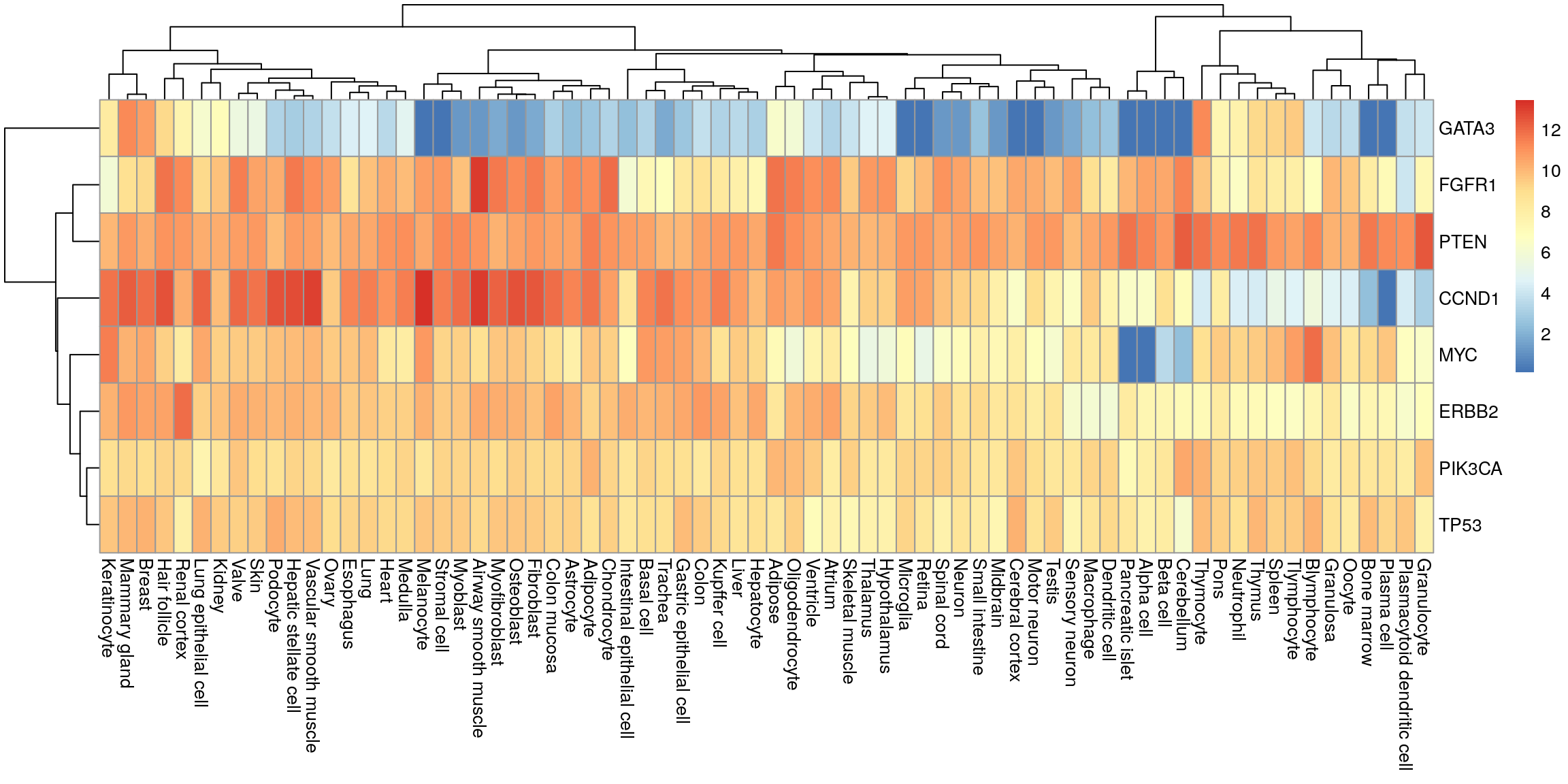
Convert to matrix and plot.
my_mat <- as.matrix(my_df_wide[, -1])
row.names(my_mat) <- my_df_wide$gene

pheatmap(my_mat)
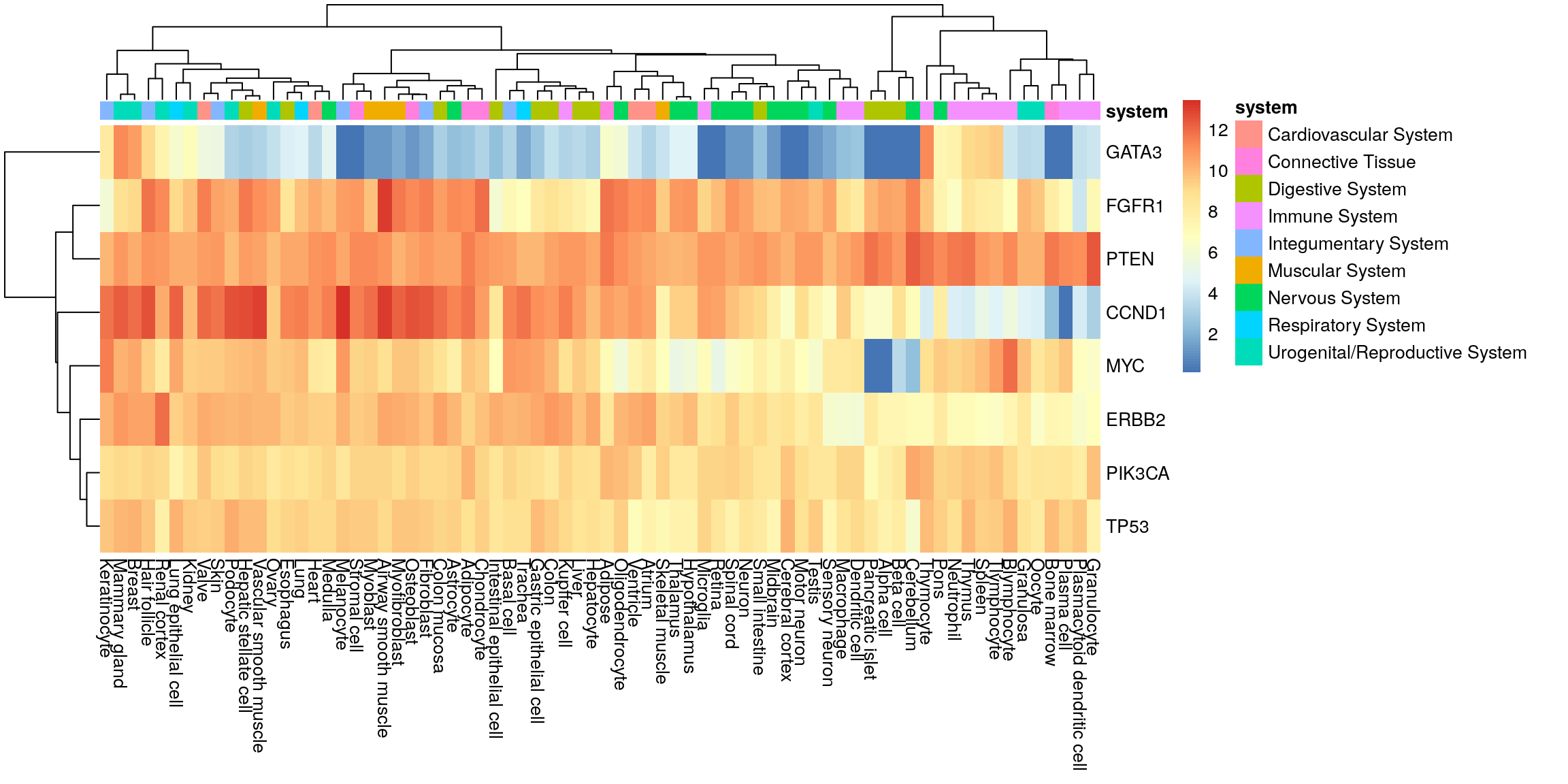
Create sample annotation.
my_order <- colnames(my_mat)

my_df |>
  dplyr::select(system, tissue) |>
  dplyr::distinct() |>
  dplyr::arrange(match(tissue, my_order)) |>
  dplyr::select(-tissue) -> sample_anno

row.names(sample_anno) <- my_order
head(sample_anno)
system
Valve Cardiovascular System
Heart Cardiovascular System
Ventricle Cardiovascular System
Atrium Cardiovascular System
Osteoblast Connective Tissue
Adipocyte Connective TissueHeatmap with system annotation.
pheatmap(my_mat, annotation_col = sample_anno)
Interactive heatmap.
plot_ly(
  x=colnames(my_mat),
  y=rownames(my_mat),
  z = my_mat,
  colors = colorRamp(c("green", "red")),
  type = "heatmap"
)
sessionInfo()R version 4.4.0 (2024-04-24)
Platform: x86_64-pc-linux-gnu
Running under: Ubuntu 22.04.4 LTS
Matrix products: default
BLAS: /usr/lib/x86_64-linux-gnu/openblas-pthread/libblas.so.3
LAPACK: /usr/lib/x86_64-linux-gnu/openblas-pthread/libopenblasp-r0.3.20.so; LAPACK version 3.10.0
locale:
[1] LC_CTYPE=en_US.UTF-8 LC_NUMERIC=C
[3] LC_TIME=en_US.UTF-8 LC_COLLATE=en_US.UTF-8
[5] LC_MONETARY=en_US.UTF-8 LC_MESSAGES=en_US.UTF-8
[7] LC_PAPER=en_US.UTF-8 LC_NAME=C
[9] LC_ADDRESS=C LC_TELEPHONE=C
[11] LC_MEASUREMENT=en_US.UTF-8 LC_IDENTIFICATION=C
time zone: Etc/UTC
tzcode source: system (glibc)
attached base packages:
[1] stats graphics grDevices utils datasets methods base
other attached packages:
[1] plotly_4.10.4 ggplot2_3.5.1 pheatmap_1.0.12 workflowr_1.7.1
loaded via a namespace (and not attached):
[1] gtable_0.3.5 xfun_0.44 bslib_0.7.0 htmlwidgets_1.6.4
[5] processx_3.8.4 callr_3.7.6 tzdb_0.4.0 crosstalk_1.2.1
[9] vctrs_0.6.5 tools_4.4.0 ps_1.7.6 generics_0.1.3
[13] parallel_4.4.0 tibble_3.2.1 fansi_1.0.6 highr_0.11
[17] pkgconfig_2.0.3 data.table_1.15.4 RColorBrewer_1.1-3 lifecycle_1.0.4
[21] compiler_4.4.0 farver_2.1.2 stringr_1.5.1 git2r_0.33.0
[25] munsell_0.5.1 getPass_0.2-4 httpuv_1.6.15 htmltools_0.5.8.1
[29] sass_0.4.9 yaml_2.3.8 lazyeval_0.2.2 later_1.3.2
[33] pillar_1.9.0 crayon_1.5.2 jquerylib_0.1.4 whisker_0.4.1
[37] tidyr_1.3.1 cachem_1.1.0 tidyselect_1.2.1 digest_0.6.35
[41] stringi_1.8.4 dplyr_1.1.4 purrr_1.0.2 labeling_0.4.3
[45] rprojroot_2.0.4 fastmap_1.2.0 grid_4.4.0 colorspace_2.1-0
[49] cli_3.6.2 magrittr_2.0.3 utf8_1.2.4 readr_2.1.5
[53] withr_3.0.0 scales_1.3.0 promises_1.3.0 bit64_4.0.5
[57] rmarkdown_2.27 httr_1.4.7 bit_4.0.5 hms_1.1.3
[61] evaluate_0.24.0 knitr_1.47 viridisLite_0.4.2 rlang_1.1.4
[65] Rcpp_1.0.12 glue_1.7.0 rstudioapi_0.16.0 vroom_1.6.5
[69] jsonlite_1.8.8 R6_2.5.1 fs_1.6.4