PCA with DESeq2
2025-04-01
Last updated: 2025-04-01
Checks: 7 0
Knit directory: muse/
This reproducible R Markdown analysis was created with workflowr (version 1.7.1). The Checks tab describes the reproducibility checks that were applied when the results were created. The Past versions tab lists the development history.
Great! Since the R Markdown file has been committed to the Git repository, you know the exact version of the code that produced these results.
Great job! The global environment was empty. Objects defined in the global environment can affect the analysis in your R Markdown file in unknown ways. For reproduciblity it’s best to always run the code in an empty environment.
The command set.seed(20200712) was run prior to running
the code in the R Markdown file. Setting a seed ensures that any results
that rely on randomness, e.g. subsampling or permutations, are
reproducible.
Great job! Recording the operating system, R version, and package versions is critical for reproducibility.
Nice! There were no cached chunks for this analysis, so you can be confident that you successfully produced the results during this run.
Great job! Using relative paths to the files within your workflowr project makes it easier to run your code on other machines.
Great! You are using Git for version control. Tracking code development and connecting the code version to the results is critical for reproducibility.
The results in this page were generated with repository version d1f7ed3. See the Past versions tab to see a history of the changes made to the R Markdown and HTML files.
Note that you need to be careful to ensure that all relevant files for
the analysis have been committed to Git prior to generating the results
(you can use wflow_publish or
wflow_git_commit). workflowr only checks the R Markdown
file, but you know if there are other scripts or data files that it
depends on. Below is the status of the Git repository when the results
were generated:
Ignored files:
    Ignored:    .Rproj.user/
    Ignored:    data/1M_neurons_filtered_gene_bc_matrices_h5.h5
    Ignored:    data/293t/
    Ignored:    data/293t_3t3_filtered_gene_bc_matrices.tar.gz
    Ignored:    data/293t_filtered_gene_bc_matrices.tar.gz
    Ignored:    data/5k_Human_Donor1_PBMC_3p_gem-x_5k_Human_Donor1_PBMC_3p_gem-x_count_sample_filtered_feature_bc_matrix.h5
    Ignored:    data/5k_Human_Donor2_PBMC_3p_gem-x_5k_Human_Donor2_PBMC_3p_gem-x_count_sample_filtered_feature_bc_matrix.h5
    Ignored:    data/5k_Human_Donor3_PBMC_3p_gem-x_5k_Human_Donor3_PBMC_3p_gem-x_count_sample_filtered_feature_bc_matrix.h5
    Ignored:    data/5k_Human_Donor4_PBMC_3p_gem-x_5k_Human_Donor4_PBMC_3p_gem-x_count_sample_filtered_feature_bc_matrix.h5
    Ignored:    data/97516b79-8d08-46a6-b329-5d0a25b0be98.h5ad
    Ignored:    data/Parent_SC3v3_Human_Glioblastoma_filtered_feature_bc_matrix.tar.gz
    Ignored:    data/brain_counts/
    Ignored:    data/cl.obo
    Ignored:    data/cl.owl
    Ignored:    data/jurkat/
    Ignored:    data/jurkat:293t_50:50_filtered_gene_bc_matrices.tar.gz
    Ignored:    data/jurkat_293t/
    Ignored:    data/jurkat_filtered_gene_bc_matrices.tar.gz
    Ignored:    data/pbmc20k/
    Ignored:    data/pbmc20k_seurat/
    Ignored:    data/pbmc3k/
    Ignored:    data/pbmc3k_seurat.rds
    Ignored:    data/pbmc4k_filtered_gene_bc_matrices.tar.gz
    Ignored:    data/pbmc_1k_v3_filtered_feature_bc_matrix.h5
    Ignored:    data/pbmc_1k_v3_raw_feature_bc_matrix.h5
    Ignored:    data/refdata-gex-GRCh38-2020-A.tar.gz
    Ignored:    data/seurat_1m_neuron.rds
    Ignored:    data/t_3k_filtered_gene_bc_matrices.tar.gz
    Ignored:    r_packages_4.4.1/

Untracked files:
    Untracked:  analysis/bioc_scrnaseq.Rmd
    Untracked:  rsem.merged.gene_counts.tsv
Note that any generated files, e.g. HTML, png, CSS, etc., are not included in this status report because it is ok for generated content to have uncommitted changes.
These are the previous versions of the repository in which changes were
made to the R Markdown (analysis/gene_exp_pca.Rmd) and HTML
(docs/gene_exp_pca.html) files. If you’ve configured a
remote Git repository (see ?wflow_git_remote), click on the
hyperlinks in the table below to view the files as they were in that
past version.
| File | Version | Author | Date | Message |
|---|---|---|---|---|
| Rmd | d1f7ed3 | Dave Tang | 2025-04-01 | Aesthetics |
| html | bbeb9ad | Dave Tang | 2025-04-01 | Build site. |
| Rmd | 5bbd819 | Dave Tang | 2025-04-01 | Show only the head of data |
| html | c9c5f07 | Dave Tang | 2025-04-01 | Build site. |
| Rmd | cf5f5ca | Dave Tang | 2025-04-01 | PCA using DESeq2 |
DESeq2 is used to:
Estimate variance-mean dependence in count data from high-throughput sequencing assays and test for differential expression based on a model using the negative binomial distribution.
Installation
Install using BiocManager::install().
if (!require("BiocManager", quietly = TRUE))
  install.packages("BiocManager")

BiocManager::install("DESeq2")
Package version.
packageVersion("DESeq2")[1] '1.46.0'Count table
https://zenodo.org/records/13970886.
my_url <- 'https://zenodo.org/records/13970886/files/rsem.merged.gene_counts.tsv?download=1'
my_file <- 'rsem.merged.gene_counts.tsv'

if(file.exists(my_file) == FALSE){
  download.file(url = my_url, destfile = my_file)
}

gene_counts <- read_tsv("rsem.merged.gene_counts.tsv", show_col_types = FALSE)
head(gene_counts)
# A tibble: 6 × 10
gene_id `transcript_id(s)` ERR160122 ERR160123 ERR160124 ERR164473 ERR164550
<chr> <chr> <dbl> <dbl> <dbl> <dbl> <dbl>
1 ENSG0000… ENST00000373020,E… 2 6 5 374 1637
2 ENSG0000… ENST00000373031,E… 19 40 28 0 1
3 ENSG0000… ENST00000371582,E… 268. 274. 429. 489 637
4 ENSG0000… ENST00000367770,E… 360. 449. 566. 363. 606.
5 ENSG0000… ENST00000286031,E… 156. 185. 265. 85.4 312.
6 ENSG0000… ENST00000374003,E… 24 23 40 1181 423
# ℹ 3 more variables: ERR164551 <dbl>, ERR164552 <dbl>, ERR164554 <dbl>Metadata.
tibble::tribble(
  ~sample, ~run_id, ~group,
  "C2_norm", "ERR160122", "normal",
  "C3_norm", "ERR160123", "normal",
  "C5_norm", "ERR160124", "normal",
  "C1_norm", "ERR164473", "normal",
  "C1_cancer", "ERR164550", "cancer",
  "C2_cancer", "ERR164551", "cancer",
  "C3_cancer", "ERR164552", "cancer",
  "C5_cancer", "ERR164554", "cancer"
) -> my_metadata

my_metadata$group <- factor(my_metadata$group, levels = c('normal', 'cancer'))
Matrix.
gene_counts |>
  dplyr::select(starts_with("ERR")) |>
  mutate(across(everything(), as.integer)) |>
  as.matrix() -> gene_counts_mat

row.names(gene_counts_mat) <- gene_counts$gene_id

idx <- match(colnames(gene_counts_mat), my_metadata$run_id)
colnames(gene_counts_mat) <- my_metadata$sample[idx]

tail(gene_counts_mat)
C2_norm C3_norm C5_norm C1_norm C1_cancer C2_cancer C3_cancer
ENSG00000293594 0 0 0 0 0 0 0
ENSG00000293595 3 5 3 0 0 0 0
ENSG00000293596 0 0 0 0 0 0 0
ENSG00000293597 1 2 11 1 2 3 1
ENSG00000293599 2 0 1 0 1 2 0
ENSG00000293600 45 59 85 561 789 1099 701
C5_cancer
ENSG00000293594 0
ENSG00000293595 0
ENSG00000293596 0
ENSG00000293597 2
ENSG00000293599 0
ENSG00000293600 845PCA
Create DESeqDataSet object.
lung_cancer <- DESeqDataSetFromMatrix(
  countData = gene_counts_mat,
  colData   = my_metadata,
  design    = ~ group
)
lung_cancer
class: DESeqDataSet
dim: 63140 8
metadata(1): version
assays(1): counts
rownames(63140): ENSG00000000003 ENSG00000000005 ... ENSG00000293599
ENSG00000293600
rowData names(0):
colnames(8): C2_norm C3_norm ... C3_cancer C5_cancer
colData names(3): sample run_id groupQuickly estimate dispersion trend and apply a variance stabilizing transformation.
pas_vst <- vst(lung_cancer)
pas_vst
class: DESeqTransform
dim: 63140 8
metadata(1): version
assays(1): ''
rownames(63140): ENSG00000000003 ENSG00000000005 ... ENSG00000293599
ENSG00000293600
rowData names(4): baseMean baseVar allZero dispFit
colnames(8): C2_norm C3_norm ... C3_cancer C5_cancer
colData names(4): sample run_id group sizeFactorPlot PCA.
plotPCA(pas_vst, intgroup = "group") +
  theme_minimal()
using ntop=500 top features by variance
| Version | Author | Date |
|---|---|---|
| c9c5f07 | Dave Tang | 2025-04-01 |
PCA data.
pca_data <- plotPCA(pas_vst, intgroup = "group", returnData = TRUE)using ntop=500 top features by variancepca_data PC1 PC2 group group.1 name
C2_norm -117.37808 7.0149036 normal normal C2_norm
C3_norm -116.03913 -13.2708426 normal normal C3_norm
C5_norm -115.34425 6.2593420 normal normal C5_norm
C1_norm 69.82117 0.8856676 normal normal C1_norm
C1_cancer 67.53316 -2.1774785 cancer cancer C1_cancer
C2_cancer 70.13468 0.7640921 cancer cancer C2_cancer
C3_cancer 70.50438 0.1610337 cancer cancer C3_cancer
C5_cancer 70.76807 0.3632821 cancer cancer C5_cancerplotPCA_copied = function(object, intgroup="condition", ntop=500, returnData=FALSE, pcsToUse=1:2){
message(paste0("using ntop=",ntop," top features by variance"))
# calculate the variance for each gene
rv <- rowVars(assay(object))
# select the ntop genes by variance
select <- order(rv, decreasing=TRUE)[seq_len(min(ntop, length(rv)))]
# perform a PCA on the data in assay(x) for the selected genes
pca <- prcomp(t(assay(object)[select,]))
# the contribution to the total variance for each component
percentVar <- pca$sdev^2 / sum( pca$sdev^2 )
if (!all(intgroup %in% names(colData(object)))) {
stop("the argument 'intgroup' should specify columns of colData(dds)")
}
# add the intgroup factors together to create a new grouping factor
group <- if (length(intgroup) > 1) {
intgroup.df <- as.data.frame(colData(object)[, intgroup, drop=FALSE])
factor(apply( intgroup.df, 1, paste, collapse=":"))
} else {
colData(object)[[intgroup]]
}
# assembly the data for the plot
pcs <- paste0("PC", pcsToUse)
d <- data.frame(V1=pca$x[,pcsToUse[1]],
V2=pca$x[,pcsToUse[2]],
group=group, name=colnames(object), colData(object))
colnames(d)[1:2] <- pcs
if (returnData) {
attr(d, "percentVar") <- percentVar[pcsToUse]
return(d)
}
ggplot(data=d, aes_string(x=pcs[1], y=pcs[2], color="group")) +
geom_point(size=3) +
xlab(paste0(pcs[1],": ",round(percentVar[pcsToUse[1]] * 100),"% variance")) +
ylab(paste0(pcs[2],": ",round(percentVar[pcsToUse[2]] * 100),"% variance")) +
coord_fixed()
}Plot using the copied function.
plotPCA_copied(pas_vst, intgroup = "group") +
  theme_minimal()
using ntop=500 top features by varianceWarning: `aes_string()` was deprecated in ggplot2 3.0.0.
ℹ Please use tidy evaluation idioms with `aes()`.
ℹ See also `vignette("ggplot2-in-packages")` for more information.
This warning is displayed once every 8 hours.
Call `lifecycle::last_lifecycle_warnings()` to see where this warning was
generated.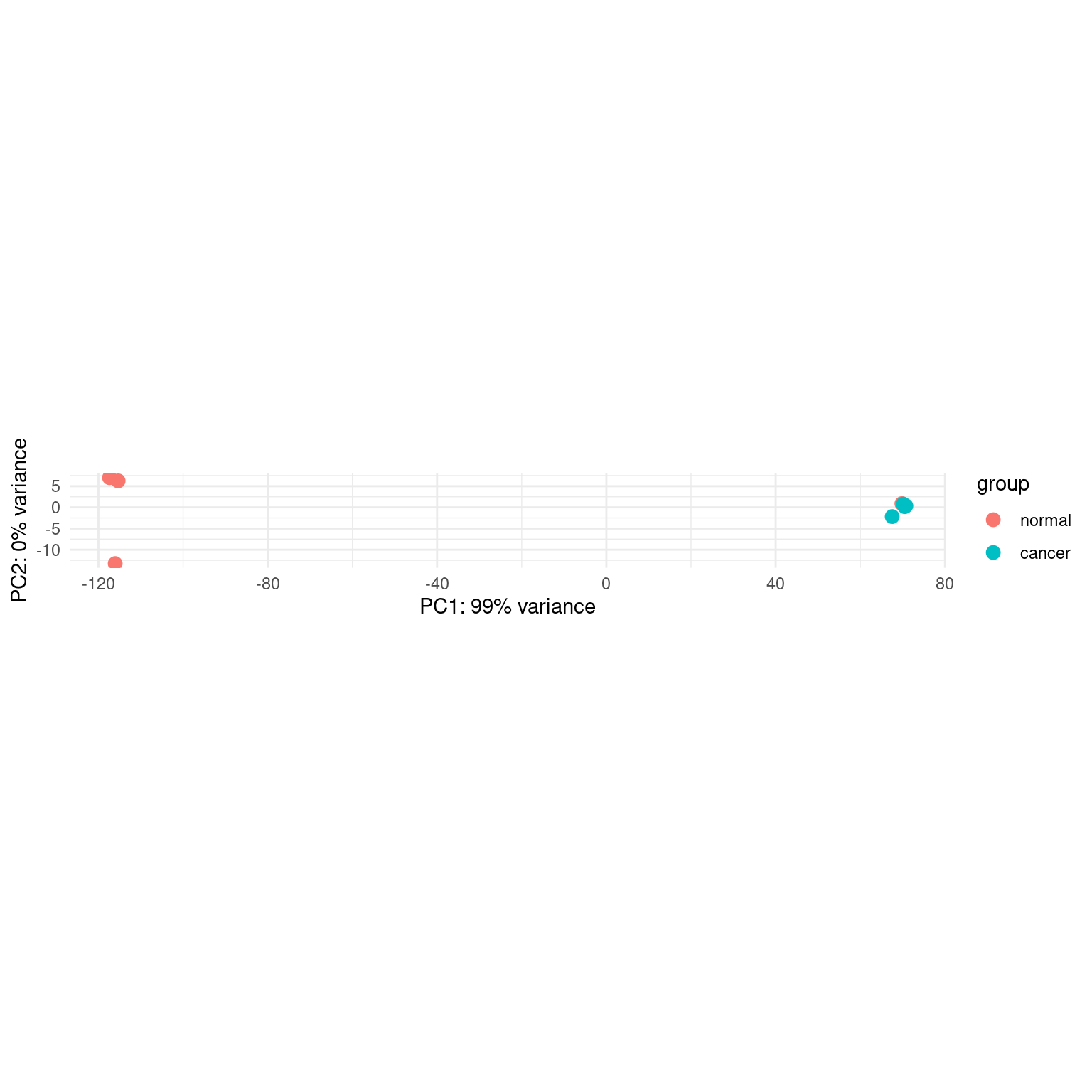
| Version | Author | Date |
|---|---|---|
| c9c5f07 | Dave Tang | 2025-04-01 |
Perform PCA as per plotPCA().
# calculate the variance for each gene
rv <- rowVars(assay(pas_vst))
head(rv)
ENSG00000000003 ENSG00000000005 ENSG00000000419 ENSG00000000457 ENSG00000000460
6.3038555 3.4528327 0.1236461 0.5966854 1.0711842
ENSG00000000938
3.6559005 # select the ntop genes by variance
ntop <- 500
topgenes <- order(rv, decreasing=TRUE)[seq_len(min(ntop, length(rv)))]
head(topgenes)[1] 12679 12446 12359 20116 53333 8411# perform a PCA on the data in assay(x) for the selected genes
pca <- prcomp(t(assay(pas_vst)[topgenes,]))Loadings are the coefficients that define how strongly each genes contributes to a principal component (PC).
loadings <- pca$rotation
loadings[1:10, 1:2]
PC1 PC2
ENSG00000169876 -0.06639949 0.008294131
ENSG00000168878 0.06304686 0.005076416
ENSG00000168484 0.05002038 0.117877848
ENSG00000205277 -0.05947887 0.023446665
ENSG00000275969 -0.05923209 0.013935605
ENSG00000143520 -0.05881607 0.007613250
ENSG00000087086 0.05824667 0.016638253
ENSG00000204849 -0.05843500 0.001321622
ENSG00000276040 -0.05730797 0.013343573
ENSG00000185775 -0.05689974 -0.001037869Squared loadings represent how much variance of each PC is attributable to each variable.
contribution <- loadings^2
contribution[1:10, 1:2]
PC1 PC2
ENSG00000169876 0.004408893 6.879261e-05
ENSG00000168878 0.003974907 2.577000e-05
ENSG00000168484 0.002502039 1.389519e-02
ENSG00000205277 0.003537736 5.497461e-04
ENSG00000275969 0.003508441 1.942011e-04
ENSG00000143520 0.003459330 5.796158e-05
ENSG00000087086 0.003392674 2.768315e-04
ENSG00000204849 0.003414650 1.746686e-06
ENSG00000276040 0.003284204 1.780509e-04
ENSG00000185775 0.003237580 1.077171e-06Gene contributing most to PC1.
sort(contribution[, 1], decreasing = TRUE) |> head()ENSG00000169876 ENSG00000168878 ENSG00000205277 ENSG00000275969 ENSG00000143520
0.004408893 0.003974907 0.003537736 0.003508441 0.003459330
ENSG00000204849
0.003414650 Note that the order is similar, because plotPCA()
already sorted the genes by their variance!
sessionInfo()R version 4.4.1 (2024-06-14)
Platform: x86_64-pc-linux-gnu
Running under: Ubuntu 22.04.5 LTS
Matrix products: default
BLAS: /usr/lib/x86_64-linux-gnu/openblas-pthread/libblas.so.3
LAPACK: /usr/lib/x86_64-linux-gnu/openblas-pthread/libopenblasp-r0.3.20.so; LAPACK version 3.10.0
locale:
[1] LC_CTYPE=en_US.UTF-8 LC_NUMERIC=C
[3] LC_TIME=en_US.UTF-8 LC_COLLATE=en_US.UTF-8
[5] LC_MONETARY=en_US.UTF-8 LC_MESSAGES=en_US.UTF-8
[7] LC_PAPER=en_US.UTF-8 LC_NAME=C
[9] LC_ADDRESS=C LC_TELEPHONE=C
[11] LC_MEASUREMENT=en_US.UTF-8 LC_IDENTIFICATION=C
time zone: Etc/UTC
tzcode source: system (glibc)
attached base packages:
[1] stats4 stats graphics grDevices utils datasets methods
[8] base
other attached packages:
[1] DESeq2_1.46.0 SummarizedExperiment_1.36.0
[3] Biobase_2.66.0 MatrixGenerics_1.18.1
[5] matrixStats_1.5.0 GenomicRanges_1.58.0
[7] GenomeInfoDb_1.42.3 IRanges_2.40.1
[9] S4Vectors_0.44.0 BiocGenerics_0.52.0
[11] lubridate_1.9.3 forcats_1.0.0
[13] stringr_1.5.1 dplyr_1.1.4
[15] purrr_1.0.2 readr_2.1.5
[17] tidyr_1.3.1 tibble_3.2.1
[19] ggplot2_3.5.1 tidyverse_2.0.0
[21] workflowr_1.7.1
loaded via a namespace (and not attached):
[1] tidyselect_1.2.1 farver_2.1.2 fastmap_1.2.0
[4] promises_1.3.2 digest_0.6.37 timechange_0.3.0
[7] lifecycle_1.0.4 processx_3.8.4 magrittr_2.0.3
[10] compiler_4.4.1 rlang_1.1.4 sass_0.4.9
[13] tools_4.4.1 utf8_1.2.4 yaml_2.3.10
[16] knitr_1.48 S4Arrays_1.6.0 labeling_0.4.3
[19] bit_4.5.0 DelayedArray_0.32.0 abind_1.4-8
[22] BiocParallel_1.40.0 withr_3.0.2 grid_4.4.1
[25] git2r_0.35.0 colorspace_2.1-1 scales_1.3.0
[28] cli_3.6.3 rmarkdown_2.28 crayon_1.5.3
[31] generics_0.1.3 rstudioapi_0.17.1 httr_1.4.7
[34] tzdb_0.4.0 cachem_1.1.0 zlibbioc_1.52.0
[37] parallel_4.4.1 XVector_0.46.0 vctrs_0.6.5
[40] Matrix_1.7-0 jsonlite_1.8.9 callr_3.7.6
[43] hms_1.1.3 bit64_4.5.2 locfit_1.5-9.12
[46] jquerylib_0.1.4 glue_1.8.0 codetools_0.2-20
[49] ps_1.8.1 stringi_1.8.4 gtable_0.3.6
[52] later_1.3.2 UCSC.utils_1.2.0 munsell_0.5.1
[55] pillar_1.10.1 htmltools_0.5.8.1 GenomeInfoDbData_1.2.13
[58] R6_2.5.1 rprojroot_2.0.4 vroom_1.6.5
[61] evaluate_1.0.1 lattice_0.22-6 highr_0.11
[64] httpuv_1.6.15 bslib_0.8.0 Rcpp_1.0.13
[67] SparseArray_1.6.2 whisker_0.4.1 xfun_0.48
[70] fs_1.6.4 getPass_0.2-4 pkgconfig_2.0.3