Seurat v4 versus v5
2025-03-11
Last updated: 2025-03-11
Checks: 7 0
Knit directory: muse/
This reproducible R Markdown analysis was created with workflowr (version 1.7.1). The Checks tab describes the reproducibility checks that were applied when the results were created. The Past versions tab lists the development history.
Great! Since the R Markdown file has been committed to the Git repository, you know the exact version of the code that produced these results.
Great job! The global environment was empty. Objects defined in the global environment can affect the analysis in your R Markdown file in unknown ways. For reproduciblity it’s best to always run the code in an empty environment.
The command set.seed(20200712) was run prior to running
the code in the R Markdown file. Setting a seed ensures that any results
that rely on randomness, e.g. subsampling or permutations, are
reproducible.
Great job! Recording the operating system, R version, and package versions is critical for reproducibility.
Nice! There were no cached chunks for this analysis, so you can be confident that you successfully produced the results during this run.
Great job! Using relative paths to the files within your workflowr project makes it easier to run your code on other machines.
Great! You are using Git for version control. Tracking code development and connecting the code version to the results is critical for reproducibility.
The results in this page were generated with repository version 4688c40. See the Past versions tab to see a history of the changes made to the R Markdown and HTML files.
Note that you need to be careful to ensure that all relevant files for
the analysis have been committed to Git prior to generating the results
(you can use wflow_publish or
wflow_git_commit). workflowr only checks the R Markdown
file, but you know if there are other scripts or data files that it
depends on. Below is the status of the Git repository when the results
were generated:
Ignored files:
    Ignored:    .Rproj.user/
    Ignored:    data/1M_neurons_filtered_gene_bc_matrices_h5.h5
    Ignored:    data/293t/
    Ignored:    data/293t_3t3_filtered_gene_bc_matrices.tar.gz
    Ignored:    data/293t_filtered_gene_bc_matrices.tar.gz
    Ignored:    data/5k_Human_Donor1_PBMC_3p_gem-x_5k_Human_Donor1_PBMC_3p_gem-x_count_sample_filtered_feature_bc_matrix.h5
    Ignored:    data/5k_Human_Donor2_PBMC_3p_gem-x_5k_Human_Donor2_PBMC_3p_gem-x_count_sample_filtered_feature_bc_matrix.h5
    Ignored:    data/5k_Human_Donor3_PBMC_3p_gem-x_5k_Human_Donor3_PBMC_3p_gem-x_count_sample_filtered_feature_bc_matrix.h5
    Ignored:    data/5k_Human_Donor4_PBMC_3p_gem-x_5k_Human_Donor4_PBMC_3p_gem-x_count_sample_filtered_feature_bc_matrix.h5
    Ignored:    data/97516b79-8d08-46a6-b329-5d0a25b0be98.h5ad
    Ignored:    data/Parent_SC3v3_Human_Glioblastoma_filtered_feature_bc_matrix.tar.gz
    Ignored:    data/brain_counts/
    Ignored:    data/cl.obo
    Ignored:    data/cl.owl
    Ignored:    data/jurkat/
    Ignored:    data/jurkat:293t_50:50_filtered_gene_bc_matrices.tar.gz
    Ignored:    data/jurkat_293t/
    Ignored:    data/jurkat_filtered_gene_bc_matrices.tar.gz
    Ignored:    data/pbmc20k/
    Ignored:    data/pbmc20k_seurat/
    Ignored:    data/pbmc3k/
    Ignored:    data/pbmc3k_seurat.rds
    Ignored:    data/pbmc4k_filtered_gene_bc_matrices.tar.gz
    Ignored:    data/pbmc_1k_v3_filtered_feature_bc_matrix.h5
    Ignored:    data/pbmc_1k_v3_raw_feature_bc_matrix.h5
    Ignored:    data/refdata-gex-GRCh38-2020-A.tar.gz
    Ignored:    data/seurat_1m_neuron.rds
    Ignored:    data/t_3k_filtered_gene_bc_matrices.tar.gz
    Ignored:    r_packages_4.4.1/

Untracked files:
    Untracked:  analysis/bioc_scrnaseq.Rmd
Note that any generated files, e.g. HTML, png, CSS, etc., are not included in this status report because it is ok for generated content to have uncommitted changes.
These are the previous versions of the repository in which changes were
made to the R Markdown (analysis/seurat_v4_vs_v5.Rmd) and
HTML (docs/seurat_v4_vs_v5.html) files. If you’ve
configured a remote Git repository (see ?wflow_git_remote),
click on the hyperlinks in the table below to view the files as they
were in that past version.
| File | Version | Author | Date | Message |
|---|---|---|---|---|
| Rmd | 4688c40 | Dave Tang | 2025-03-11 | Overdispersion exists in all scRNA-seq datasets if sufficiently sequenced |
| html | 6248d96 | Dave Tang | 2025-03-11 | Build site. |
| Rmd | d47858c | Dave Tang | 2025-03-11 | Pearson residuals |
| html | 747fe3f | Dave Tang | 2025-03-11 | Build site. |
| Rmd | 4aacb58 | Dave Tang | 2025-03-11 | Error versus variance |
| html | fc7e28d | Dave Tang | 2025-03-11 | Build site. |
| Rmd | 6139935 | Dave Tang | 2025-03-11 | Introduction to modelling variance |
| html | 94116b1 | Dave Tang | 2025-03-10 | Build site. |
| Rmd | 4c187b3 | Dave Tang | 2025-03-10 | Data layer |
| html | 0d51a69 | Dave Tang | 2025-03-10 | Build site. |
| Rmd | 48661b3 | Dave Tang | 2025-03-10 | Seurat version 4 vs. 5 |
sctransform
The paper Comparison and evaluation of statistical error models for scRNA-seq is the basis for the default approach used in Seurat version 5. The following is text from the paper:
- Heterogeneity in single-cell RNA-seq (scRNA-seq) data is driven by
multiple sources, including biological variation in cellular state as
well as technical variation introduced during experimental processing.
Deconvolving these effects is a key challenge for preprocessing
workflows.
- Separating biological heterogeneity across cells that corresponds to differences in cell type and state from alternative sources of variation represents a key analytical challenge in the normalization and preprocessing of single-cell RNA-seq data.
- Data normalization aims to adjust for differences in cellular sequencing depth, which collectively arise from fluctuations in cellular RNA content, efficiency in lysis and reverse transcription, and stochastic sampling during next-generation sequencing.
- Variance stabilization aims to address the confounding relationship between gene abundance and gene variance, and to ensure that both lowly and highly expressed genes can contribute to the downstream definition of cellular state.
Using statistical models like Generalised Linear Models:
- Two recent studies proposed to use generalized linear models (GLMs), where cellular sequencing depth was included as a covariate, as part of scRNA-seq preprocessing workflows.
- The sctransform approach utilizes the Pearson residuals from negative binomial regression as input to standard dimensional reduction techniques, while GLM-PCA focuses on a generalized version of principal component analysis (PCA) for data with Poisson-distributed errors.
- More broadly, multiple techniques aim to learn a latent state that captures biologically relevant cellular heterogeneity using either matrix factorization or neural networks, alongside a defined error model that describes the variation that is not captured by the latent space.
If a regression model doesn’t fully explain variability, the residuals might contain structure that another technique can capture to uncover hidden patterns. For example, if a regression model captures main trends, applying Principal Component Analysis (PCA) on residuals can find underlying structures in the unexplained variance. Another use case can be clustering on residuals to group data points based on deviations from a model.
Parameterising statistical models:
- Likelihood-based approaches require an explicit definition of a statistical error model for scRNA-seq, and there is little consensus on how to define or parameterize this model.
- Multiple groups have utilized a Poisson error model but others argue that the data exhibit evidence of overdispersion, requiring the use of a negative-binomial (NB) distribution.
- Methods that assume a NB distribution have different methods to
parameterize their model.
- A recent study argued that fixing the NB inverse overdispersion parameter \(\theta\) to a single value is an appropriate estimate of technical overdispersion for all genes in all scRNA-seq datasets, while others propose learning unique parameter values for each gene in each dataset.
- This lack of consensus is further exemplified by the scvi-tools suite, which supports nine different methods for parameterizing error models.
- The purpose of this error model is to describe and quantify heterogeneity that is not captured by biologically relevant differences in cell state, and highlights a specific question: How can we model the observed variation in gene expression for an scRNA-seq experiment conducted on a biologically “homogeneous” population?
Error and variance
- Error modeling refers to capturing and understanding the uncertainty, randomness, and deviations in data or predictions. Error is not exactly synonymous with variance but they are related.
- Errors arise from:
- Randomness: unavoidable variability in data, e.g., measurement noise and natural fluctuations
- Model Imperfections: due to missing information or incorrect model assumptions.
- Statistical models, like regression, often include an error term \(\epsilon\) to account for these uncertainties:
\[ Y = f(X) + \epsilon \]
where \(\epsilon\) captures random fluctuations or unknown influences.
While error contributes to variance, they are distinct:
- Error: The deviation of an observation from the model’s predicted value.
- Variance: A statistical measure of how much values deviate from their mean (spread of data).
Errors can be random (causing variability) or systematic (bias), but variance is a quantification of dispersion.
- In regression, we separate variance into explained variance (by the model) and unexplained variance (error).
- Error variance \(\sigma^2\) is modeled to improve predictions and uncertainty estimation.
- For a negative binomial regression model, the Pearson residual \(r_i\) for observation \(i\) is given by:
\[ r_i = \frac{y_i - \hat{y}_i}{\sqrt{\text{Var}(y_i)}} \]
where:
* \(y_i\) = observed count
* \(\hat{y}_i\) = predicted mean
(expected value under the model)
* \(\text{Var}(y_i)\) = model-estimated
variance of \(y_i\)
- Unlike Poisson regression (where \(\text{Var}(y) = \hat{y}\)), the negative binomial model accounts for overdispersion using a dispersion parameter \(\theta\), and the variance is:
\[ \text{Var}(y_i) = \hat{y}_i + \frac{\hat{y}_i^2}{\theta} \]
This means the variance grows faster than the mean, making negative binomial regression suitable when count data has extra variability.
- Pearson residuals can be used for:
- Standardized measure - Large residuals (\(|r_i| > 2\)) may indicate poor model fit.
- Overdispersion check - If Pearson residuals systematically increase with predicted values, it suggests the model may not fully account for overdispersion.
- Model diagnostics - Residual plots help assess whether assumptions (e.g., correct functional form) hold.
Pearson residuals focus on variance-adjusted differences and deviance residuals come from likelihood-based goodness-of-fit measures. They both help diagnose model fit, but deviance residuals tend to emphasise extreme deviations more. Pearson residuals in negative binomial regression are useful for model diagnostics, particularly for checking overdispersion and assessing fit.
Seurat object
Import raw pbmc3k dataset from my server.
seurat_obj <- readRDS(url("https://davetang.org/file/pbmc3k_seurat.rds", "rb"))
seurat_obj
An object of class Seurat
32738 features across 2700 samples within 1 assay
Active assay: RNA (32738 features, 0 variable features)
1 layer present: countsFilter.
pbmc3k <- CreateSeuratObject(
  counts = seurat_obj@assays$RNA$counts,
  min.cells = 3,
  min.features = 200,
  project = "pbmc3k"
)
pbmc3k
An object of class Seurat
13714 features across 2700 samples within 1 assay
Active assay: RNA (13714 features, 0 variable features)
1 layer present: countsSeurat workflows
Process with the Seurat 4 workflow.
seurat_wf_v4 <- function(seurat_obj, scale_factor = 1e4, num_features = 2000, num_pcs = 30, cluster_res = 0.5, debug_flag = FALSE){

  seurat_obj <- NormalizeData(seurat_obj, normalization.method = "LogNormalize", scale.factor = scale_factor, verbose = debug_flag)
  seurat_obj <- FindVariableFeatures(seurat_obj, selection.method = 'vst', nfeatures = num_features, verbose = debug_flag)
  seurat_obj <- ScaleData(seurat_obj, verbose = debug_flag)
  seurat_obj <- RunPCA(seurat_obj, verbose = debug_flag)
  seurat_obj <- RunUMAP(seurat_obj, dims = 1:num_pcs, verbose = debug_flag)
  seurat_obj <- FindNeighbors(seurat_obj, dims = 1:num_pcs, verbose = debug_flag)
  seurat_obj <- FindClusters(seurat_obj, resolution = cluster_res, verbose = debug_flag)

  seurat_obj
}

pbmc3k_v4 <- seurat_wf_v4(pbmc3k)
Warning: The default method for RunUMAP has changed from calling Python UMAP via reticulate to the R-native UWOT using the cosine metric
To use Python UMAP via reticulate, set umap.method to 'umap-learn' and metric to 'correlation'
This message will be shown once per sessionpbmc3k_v4An object of class Seurat
13714 features across 2700 samples within 1 assay
Active assay: RNA (13714 features, 2000 variable features)
3 layers present: counts, data, scale.data
2 dimensional reductions calculated: pca, umapUMAP.
DimPlot(pbmc3k_v4, reduction = "umap")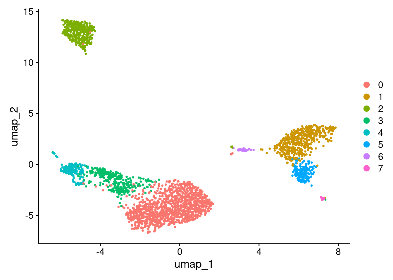
| Version | Author | Date |
|---|---|---|
| 0d51a69 | Dave Tang | 2025-03-10 |
seurat_wf_v5 <- function(seurat_obj, scale_factor = 1e4, num_features = 2000, num_pcs = 30, cluster_res = 0.5, debug_flag = FALSE){

  seurat_obj <- SCTransform(seurat_obj, verbose = debug_flag)
  seurat_obj <- RunPCA(seurat_obj, verbose = debug_flag)
  seurat_obj <- RunUMAP(seurat_obj, dims = 1:num_pcs, verbose = debug_flag)
  seurat_obj <- FindNeighbors(seurat_obj, dims = 1:num_pcs, verbose = debug_flag)
  seurat_obj <- FindClusters(seurat_obj, resolution = cluster_res, verbose = debug_flag)

  seurat_obj
}

pbmc3k_v5 <- seurat_wf_v5(pbmc3k)
pbmc3k_v5
An object of class Seurat
26286 features across 2700 samples within 2 assays
Active assay: SCT (12572 features, 3000 variable features)
3 layers present: counts, data, scale.data
1 other assay present: RNA
2 dimensional reductions calculated: pca, umapUMAP.
DimPlot(pbmc3k_v5, reduction = "umap")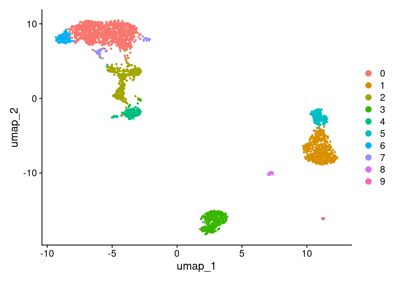
| Version | Author | Date |
|---|---|---|
| 0d51a69 | Dave Tang | 2025-03-10 |
Data layer
Version 4 store log normalised data.
colSums(pbmc3k_v4@assays$RNA$data)[1:6]AAACATACAACCAC-1 AAACATTGAGCTAC-1 AAACATTGATCAGC-1 AAACCGTGCTTCCG-1
1605.823 2027.859 2040.169 1902.960
AAACCGTGTATGCG-1 AAACGCACTGGTAC-1
1388.125 1653.061 The data layer is in the SCT assay.
colSums(pbmc3k_v5@assays$SCT$data)[1:6]AAACATACAACCAC-1 AAACATTGAGCTAC-1 AAACATTGATCAGC-1 AAACCGTGCTTCCG-1
786.2686 1024.4731 1029.3032 934.4454
AAACCGTGTATGCG-1 AAACGCACTGGTAC-1
666.1142 764.8101 Compare clustering
More granular clustering of version 4’s cluster 0 in version 5.
stopifnot(all(row.names(pbmc3k_v4@meta.data) == row.names(pbmc3k_v5@meta.data)))

table(
  pbmc3k_v4@meta.data$seurat_clusters,
  pbmc3k_v5@meta.data$seurat_clusters
)
      0   1   2   3   4   5   6   7   8   9
  0 970   0  71   2   0   0 100  44   0   0
  1   0 479   0   0   0   9   0   0   3   0
  2   1   0   0 349   0   0   0   1   0   0
  3   4   0 290   1   5   0   0   1   0   0
  4   0   0   5   6 152   0   0   0   0   0
  5   0  16   0   0   0 145   0   0   0   0
  6   0   1   0   0   0   0   0   0  31   0
  7   0   1   0   1   0   0   0   0   0  12
Appendix
More information text from the paper Comparison and evaluation of statistical error models for scRNA-seq.
Shallow sequencing masks overdispersion in scRNA-seq data
- The rationale behind a Poisson model assumes that homogeneous cells express mRNA molecules for a given gene at a fixed underlying rate, and the variation in scRNA-seq results specifically from a stochastic sampling of mRNA molecules, for example due to inefficiencies in reverse transcription and PCR, combined with incomplete molecular sampling during DNA sequencing
- While the Poisson distribution is well suited to capture variation
driven by stochastic technical loss and sampling noise, it cannot
capture other sources of biological heterogeneity between cells that are
not driven by changes in cell state, for example, intrinsic variation
caused by stochastic transcriptional bursts.
- These fluctuations would cause scRNA-seq data to deviate from Poisson statistics, exhibiting overdispersion.
- To assess whether scRNA-seq datasets follow the Poisson distribution, the authors performed a goodness-of-fit test, independently modeling the observed counts for each gene to be Poisson distributed, while accounting for differences in sequencing depth between individual cells.
- In each of the 59 datasets analysed, genes exhibiting Poisson
variation were overwhelmingly lowly expressed compared to genes that
were overdispersed.
- Moreover, when comparing results for cell-line datasets where we expect low levels of variation in cell state, we found that the global fraction of genes deviating from a Poisson distribution was correlated with the average sequencing depth of the dataset.
- The results suggest that scRNA-seq datasets commonly exhibit biological variation that exceeds Poisson sampling, but that the statistical power to detect these fluctuations requires sufficient sequencing depth.
- After downsampling, only 0.5% genes failed the Poisson goodness-of-fit test, demonstrating that reducing cellular sequencing depth can artificially create the appearance of Poisson variation.
- The authors conclude that the Poisson error model may represent an acceptable approximation for scRNA-seq datasets with shallow sequencing, but as the sensitivity of molecular profiling continues to increase, error models that allow for overdispersion are required for scRNA-seq analysis.
sessionInfo()R version 4.4.1 (2024-06-14)
Platform: x86_64-pc-linux-gnu
Running under: Ubuntu 22.04.5 LTS
Matrix products: default
BLAS: /usr/lib/x86_64-linux-gnu/openblas-pthread/libblas.so.3
LAPACK: /usr/lib/x86_64-linux-gnu/openblas-pthread/libopenblasp-r0.3.20.so; LAPACK version 3.10.0
locale:
[1] LC_CTYPE=en_US.UTF-8 LC_NUMERIC=C
[3] LC_TIME=en_US.UTF-8 LC_COLLATE=en_US.UTF-8
[5] LC_MONETARY=en_US.UTF-8 LC_MESSAGES=en_US.UTF-8
[7] LC_PAPER=en_US.UTF-8 LC_NAME=C
[9] LC_ADDRESS=C LC_TELEPHONE=C
[11] LC_MEASUREMENT=en_US.UTF-8 LC_IDENTIFICATION=C
time zone: Etc/UTC
tzcode source: system (glibc)
attached base packages:
[1] stats graphics grDevices utils datasets methods base
other attached packages:
[1] Seurat_5.2.1 SeuratObject_5.0.2 sp_2.2-0 lubridate_1.9.4
[5] forcats_1.0.0 stringr_1.5.1 dplyr_1.1.4 purrr_1.0.4
[9] readr_2.1.5 tidyr_1.3.1 tibble_3.2.1 ggplot2_3.5.1
[13] tidyverse_2.0.0 workflowr_1.7.1
loaded via a namespace (and not attached):
[1] RColorBrewer_1.1-3 rstudioapi_0.17.1
[3] jsonlite_1.9.1 magrittr_2.0.3
[5] spatstat.utils_3.1-2 farver_2.1.2
[7] rmarkdown_2.29 zlibbioc_1.52.0
[9] fs_1.6.5 vctrs_0.6.5
[11] ROCR_1.0-11 DelayedMatrixStats_1.28.1
[13] spatstat.explore_3.3-4 S4Arrays_1.6.0
[15] htmltools_0.5.8.1 SparseArray_1.6.2
[17] sass_0.4.9 sctransform_0.4.1
[19] parallelly_1.42.0 KernSmooth_2.23-24
[21] bslib_0.9.0 htmlwidgets_1.6.4
[23] ica_1.0-3 plyr_1.8.9
[25] plotly_4.10.4 zoo_1.8-13
[27] cachem_1.1.0 whisker_0.4.1
[29] igraph_2.1.4 mime_0.12
[31] lifecycle_1.0.4 pkgconfig_2.0.3
[33] Matrix_1.7-0 R6_2.6.1
[35] fastmap_1.2.0 GenomeInfoDbData_1.2.13
[37] MatrixGenerics_1.18.1 fitdistrplus_1.2-2
[39] future_1.34.0 shiny_1.10.0
[41] digest_0.6.37 colorspace_2.1-1
[43] S4Vectors_0.44.0 patchwork_1.3.0
[45] ps_1.9.0 rprojroot_2.0.4
[47] tensor_1.5 RSpectra_0.16-2
[49] irlba_2.3.5.1 GenomicRanges_1.58.0
[51] labeling_0.4.3 progressr_0.15.1
[53] spatstat.sparse_3.1-0 timechange_0.3.0
[55] httr_1.4.7 polyclip_1.10-7
[57] abind_1.4-8 compiler_4.4.1
[59] withr_3.0.2 fastDummies_1.7.5
[61] MASS_7.3-60.2 DelayedArray_0.32.0
[63] tools_4.4.1 lmtest_0.9-40
[65] httpuv_1.6.15 future.apply_1.11.3
[67] goftest_1.2-3 glmGamPoi_1.18.0
[69] glue_1.8.0 callr_3.7.6
[71] nlme_3.1-164 promises_1.3.2
[73] grid_4.4.1 Rtsne_0.17
[75] getPass_0.2-4 cluster_2.1.6
[77] reshape2_1.4.4 generics_0.1.3
[79] gtable_0.3.6 spatstat.data_3.1-4
[81] tzdb_0.4.0 data.table_1.17.0
[83] hms_1.1.3 XVector_0.46.0
[85] BiocGenerics_0.52.0 spatstat.geom_3.3-5
[87] RcppAnnoy_0.0.22 ggrepel_0.9.6
[89] RANN_2.6.2 pillar_1.10.1
[91] spam_2.11-1 RcppHNSW_0.6.0
[93] later_1.4.1 splines_4.4.1
[95] lattice_0.22-6 survival_3.6-4
[97] deldir_2.0-4 tidyselect_1.2.1
[99] miniUI_0.1.1.1 pbapply_1.7-2
[101] knitr_1.49 git2r_0.35.0
[103] gridExtra_2.3 IRanges_2.40.1
[105] SummarizedExperiment_1.36.0 scattermore_1.2
[107] stats4_4.4.1 xfun_0.51
[109] Biobase_2.66.0 matrixStats_1.5.0
[111] UCSC.utils_1.2.0 stringi_1.8.4
[113] lazyeval_0.2.2 yaml_2.3.10
[115] evaluate_1.0.3 codetools_0.2-20
[117] cli_3.6.4 uwot_0.2.3
[119] xtable_1.8-4 reticulate_1.41.0
[121] munsell_0.5.1 processx_3.8.6
[123] jquerylib_0.1.4 GenomeInfoDb_1.42.3
[125] Rcpp_1.0.14 globals_0.16.3
[127] spatstat.random_3.3-2 png_0.1-8
[129] spatstat.univar_3.1-2 parallel_4.4.1
[131] dotCall64_1.2 sparseMatrixStats_1.18.0
[133] listenv_0.9.1 viridisLite_0.4.2
[135] scales_1.3.0 ggridges_0.5.6
[137] crayon_1.5.3 rlang_1.1.5
[139] cowplot_1.1.3