4.10 Single cell RNA-seq differential expression with pseudobulking
2026-02-03
Last updated: 2026-02-03
Checks: 7 0
Knit directory: muse/
This reproducible R Markdown analysis was created with workflowr (version 1.7.1). The Checks tab describes the reproducibility checks that were applied when the results were created. The Past versions tab lists the development history.
Great! Since the R Markdown file has been committed to the Git repository, you know the exact version of the code that produced these results.
Great job! The global environment was empty. Objects defined in the global environment can affect the analysis in your R Markdown file in unknown ways. For reproduciblity it’s best to always run the code in an empty environment.
The command set.seed(20200712) was run prior to running
the code in the R Markdown file. Setting a seed ensures that any results
that rely on randomness, e.g. subsampling or permutations, are
reproducible.
Great job! Recording the operating system, R version, and package versions is critical for reproducibility.
Nice! There were no cached chunks for this analysis, so you can be confident that you successfully produced the results during this run.
Great job! Using relative paths to the files within your workflowr project makes it easier to run your code on other machines.
Great! You are using Git for version control. Tracking code development and connecting the code version to the results is critical for reproducibility.
The results in this page were generated with repository version 2051918. See the Past versions tab to see a history of the changes made to the R Markdown and HTML files.
Note that you need to be careful to ensure that all relevant files for
the analysis have been committed to Git prior to generating the results
(you can use wflow_publish or
wflow_git_commit). workflowr only checks the R Markdown
file, but you know if there are other scripts or data files that it
depends on. Below is the status of the Git repository when the results
were generated:
Ignored files:
    Ignored:    .Rproj.user/
    Ignored:    data/1M_neurons_filtered_gene_bc_matrices_h5.h5
    Ignored:    data/293t/
    Ignored:    data/293t_3t3_filtered_gene_bc_matrices.tar.gz
    Ignored:    data/293t_filtered_gene_bc_matrices.tar.gz
    Ignored:    data/5k_Human_Donor1_PBMC_3p_gem-x_5k_Human_Donor1_PBMC_3p_gem-x_count_sample_filtered_feature_bc_matrix.h5
    Ignored:    data/5k_Human_Donor2_PBMC_3p_gem-x_5k_Human_Donor2_PBMC_3p_gem-x_count_sample_filtered_feature_bc_matrix.h5
    Ignored:    data/5k_Human_Donor3_PBMC_3p_gem-x_5k_Human_Donor3_PBMC_3p_gem-x_count_sample_filtered_feature_bc_matrix.h5
    Ignored:    data/5k_Human_Donor4_PBMC_3p_gem-x_5k_Human_Donor4_PBMC_3p_gem-x_count_sample_filtered_feature_bc_matrix.h5
    Ignored:    data/97516b79-8d08-46a6-b329-5d0a25b0be98.h5ad
    Ignored:    data/Parent_SC3v3_Human_Glioblastoma_filtered_feature_bc_matrix.tar.gz
    Ignored:    data/brain_counts/
    Ignored:    data/cl.obo
    Ignored:    data/cl.owl
    Ignored:    data/jurkat/
    Ignored:    data/jurkat:293t_50:50_filtered_gene_bc_matrices.tar.gz
    Ignored:    data/jurkat_293t/
    Ignored:    data/jurkat_filtered_gene_bc_matrices.tar.gz
    Ignored:    data/pbmc20k/
    Ignored:    data/pbmc20k_seurat/
    Ignored:    data/pbmc3k.csv
    Ignored:    data/pbmc3k.csv.gz
    Ignored:    data/pbmc3k.h5ad
    Ignored:    data/pbmc3k/
    Ignored:    data/pbmc3k_bpcells_mat/
    Ignored:    data/pbmc3k_export.mtx
    Ignored:    data/pbmc3k_matrix.mtx
    Ignored:    data/pbmc3k_seurat.rds
    Ignored:    data/pbmc4k_filtered_gene_bc_matrices.tar.gz
    Ignored:    data/pbmc_1k_v3_filtered_feature_bc_matrix.h5
    Ignored:    data/pbmc_1k_v3_raw_feature_bc_matrix.h5
    Ignored:    data/refdata-gex-GRCh38-2020-A.tar.gz
    Ignored:    data/seurat_1m_neuron.rds
    Ignored:    data/t_3k_filtered_gene_bc_matrices.tar.gz
    Ignored:    r_packages_4.4.1/
    Ignored:    r_packages_4.5.0/

Untracked files:
    Untracked:  .claude/
    Untracked:  CLAUDE.md
    Untracked:  analysis/bioc.Rmd
    Untracked:  analysis/bioc_scrnaseq.Rmd
    Untracked:  analysis/chick_weight.Rmd
    Untracked:  analysis/likelihood.Rmd
    Untracked:  bpcells_matrix/
    Untracked:  data/Caenorhabditis_elegans.WBcel235.113.gtf.gz
    Untracked:  data/GCF_043380555.1-RS_2024_12_gene_ontology.gaf.gz
    Untracked:  data/SeuratObj.rds
    Untracked:  data/arab.rds
    Untracked:  data/astronomicalunit.csv
    Untracked:  data/femaleMiceWeights.csv
    Untracked:  data/lung_bcell.rds
    Untracked:  m3/
    Untracked:  women.json

Unstaged changes:
    Modified:   analysis/isoform_switch_analyzer.Rmd
    Modified:   analysis/linear_models.Rmd
Note that any generated files, e.g. HTML, png, CSS, etc., are not included in this status report because it is ok for generated content to have uncommitted changes.
These are the previous versions of the repository in which changes were
made to the R Markdown (analysis/edger_pb.Rmd) and HTML
(docs/edger_pb.html) files. If you’ve configured a remote
Git repository (see ?wflow_git_remote), click on the
hyperlinks in the table below to view the files as they were in that
past version.
| File | Version | Author | Date | Message |
|---|---|---|---|---|
| Rmd | 2051918 | Dave Tang | 2026-02-03 | Using a cell means model for the design matrix |
| html | 074cd66 | Dave Tang | 2026-02-03 | Build site. |
| Rmd | e760666 | Dave Tang | 2026-02-03 | Include background information |
| html | 8793f37 | Dave Tang | 2026-02-03 | Build site. |
| Rmd | 158ac67 | Dave Tang | 2026-02-03 | Pseudobulk analysis using edgeR |
Introduction
Performing differential expression (DE) analysis on scRNA-seq data presents unique challenges with the primary problem being that individual cells exhibit high variability.
Pseudobulking tries to address the issue of variability by aggregating counts from cells that share the same biological replicate (e.g., donor/sample) and cell type. This approach:
- Reduces technical noise by averaging across many cells.
- Properly accounts for biological replication at the sample level.
- Allows the use of well-established bulk RNA-seq DE methods (e.g., edgeR) that have robust statistical frameworks.
This notebook demonstrates how to perform pseudobulk differential expression analysis using edgeR, following the workflow described in Section 4.10 of the edgeR User’s Guide.
Data
The single cell RNA-seq data used in this notebook is from the human breast single cell RNA atlas generated by Pal et al. The preprocessing of the data and the complete bioinformatics analyses of the entire atlas study are described in detail in Chen et al. Most of the single cell analysis, such as dimensionality reduction and integration, were performed using Seurat. All the generated Seurat objects are publicly available on Figshare.
The Seurat object used in this notebook was downloaded directly from the website of the edgeR maintainers. This object contains breast tissue micro-environment samples from 13 individual healthy donors. This object has been subsetted to contain 10,000 cells of the total 24,751 cells from the original object.
so <- readRDS("data/SeuratObj.rds")
so
An object of class Seurat
15527 features across 10000 samples within 2 assays
Active assay: integrated (2000 features, 2000 variable features)
1 layer present: data
1 other assay present: RNA
2 dimensional reductions calculated: pca, tsneDistribution of cell counts across 13 healthy donors and 7 clusters; note that some samples don’t have cells belonging to a certain cluster.
table(so@meta.data$group, so@meta.data$seurat_clusters)
                    0   1   2   3   4   5   6
  N_0019_total    346 183 100  36  33  14   9
  N_0021_total     25 214  41   4   2   9   8
  N_0064_total     72  93  41   1   0   1   0
  N_0092_total    207 102  67  18   2  12   0
  N_0093_total    305 433 282   7  11   5  36
  N_0123_total    364 189  63  24   3  18   5
  N_0169_total    739 220 165 151 115   7  19
  N_0230.17_total 657 147 117  12  18  11   6
  N_0233_total    622 148 169  72 127  21  11
  N_0275_total     56 128  57   1   2   1   0
  N_0288_total     58 225 129   1   0   3   0
  N_0342_total    567 692 331  19   9  57  10
  N_0372_total    355 169  72  34  64   3  18
Pseudobulking
Pseudo-bulk samples are created by aggregating read counts together
for all the cells with the same combination of human donor and cluster.
Here, we generate pseudo-bulk expression profiles from the Seurat object
using the Seurat2PB() function. The human donor and cell
cluster information of the integrated single cell data is stored in the
group and seurat_clusters columns of the
meta.data component of the Seurat object.
y <- Seurat2PB(so, sample="group", cluster="seurat_clusters")
dim(y$samples)
[1] 85 5sum(table(so@meta.data$group, so@meta.data$seurat_clusters) > 0)[1] 85Counts are aggregated into samples + clusters; note that there aren’t 13 * 7 samples because as we noted in the table, some combinations have 0 counts.
colnames(y$counts) [1] "N_0019_total_cluster0" "N_0019_total_cluster1"
[3] "N_0019_total_cluster2" "N_0019_total_cluster3"
[5] "N_0019_total_cluster4" "N_0019_total_cluster5"
[7] "N_0019_total_cluster6" "N_0021_total_cluster0"
[9] "N_0021_total_cluster1" "N_0021_total_cluster2"
[11] "N_0021_total_cluster3" "N_0021_total_cluster4"
[13] "N_0021_total_cluster5" "N_0021_total_cluster6"
[15] "N_0064_total_cluster0" "N_0064_total_cluster1"
[17] "N_0064_total_cluster2" "N_0064_total_cluster3"
[19] "N_0064_total_cluster5" "N_0092_total_cluster0"
[21] "N_0092_total_cluster1" "N_0092_total_cluster2"
[23] "N_0092_total_cluster3" "N_0092_total_cluster4"
[25] "N_0092_total_cluster5" "N_0093_total_cluster0"
[27] "N_0093_total_cluster1" "N_0093_total_cluster2"
[29] "N_0093_total_cluster3" "N_0093_total_cluster4"
[31] "N_0093_total_cluster5" "N_0093_total_cluster6"
[33] "N_0123_total_cluster0" "N_0123_total_cluster1"
[35] "N_0123_total_cluster2" "N_0123_total_cluster3"
[37] "N_0123_total_cluster4" "N_0123_total_cluster5"
[39] "N_0123_total_cluster6" "N_0169_total_cluster0"
[41] "N_0169_total_cluster1" "N_0169_total_cluster2"
[43] "N_0169_total_cluster3" "N_0169_total_cluster4"
[45] "N_0169_total_cluster5" "N_0169_total_cluster6"
[47] "N_0230.17_total_cluster0" "N_0230.17_total_cluster1"
[49] "N_0230.17_total_cluster2" "N_0230.17_total_cluster3"
[51] "N_0230.17_total_cluster4" "N_0230.17_total_cluster5"
[53] "N_0230.17_total_cluster6" "N_0233_total_cluster0"
[55] "N_0233_total_cluster1" "N_0233_total_cluster2"
[57] "N_0233_total_cluster3" "N_0233_total_cluster4"
[59] "N_0233_total_cluster5" "N_0233_total_cluster6"
[61] "N_0275_total_cluster0" "N_0275_total_cluster1"
[63] "N_0275_total_cluster2" "N_0275_total_cluster3"
[65] "N_0275_total_cluster4" "N_0275_total_cluster5"
[67] "N_0288_total_cluster0" "N_0288_total_cluster1"
[69] "N_0288_total_cluster2" "N_0288_total_cluster3"
[71] "N_0288_total_cluster5" "N_0342_total_cluster0"
[73] "N_0342_total_cluster1" "N_0342_total_cluster2"
[75] "N_0342_total_cluster3" "N_0342_total_cluster4"
[77] "N_0342_total_cluster5" "N_0342_total_cluster6"
[79] "N_0372_total_cluster0" "N_0372_total_cluster1"
[81] "N_0372_total_cluster2" "N_0372_total_cluster3"
[83] "N_0372_total_cluster4" "N_0372_total_cluster5"
[85] "N_0372_total_cluster6" The total UMI counts per pseudobulk sample vary considerably, reflecting differences in the number of cells aggregated and their sequencing depth. Importantly, the minimum is greater than zero, confirming that all sample-cluster combinations retained after aggregation contain actual expression data.
summary(colSums(y$counts)) Min. 1st Qu. Median Mean 3rd Qu. Max.
1352 42181 165537 651543 776854 5011510 Filtering and normalisation
Before differential expression analysis, we apply two filtering steps to remove low-quality data that could compromise statistical inference.
Sample filtering
Pseudobulk samples with very few total counts are unreliable because they may represent too few cells or low-quality aggregations. We remove samples with fewer than 50,000 total UMI counts.
keep.samples <- y$samples$lib.size > 5e4
y <- y[, keep.samples]

dim(y$samples)
[1] 59 5Gene filtering
Genes with very low counts across samples provide little statistical
information and can adversely affect the multiple testing correction.
The filterByExpr() function implements edgeR’s recommended
filtering strategy: it keeps genes that have sufficiently large counts
to be statistically meaningful in at least some samples. By default, it
requires a gene to have at least 10 counts (min.count = 10)
in a minimum number of samples (determined by the smallest group
size).
keep.genes <- filterByExpr(y, group=y$samples$cluster)
y <- y[keep.genes, , keep=FALSE]
TMM normalisation
Trimmed Mean of M-values (TMM) normalisation corrects for compositional biases between samples. This is important because differences in library size alone don’t account for situations where a few highly-expressed genes consume a disproportionate share of sequencing reads, making other genes appear artificially down-regulated. TMM calculates scaling factors that adjust for these composition effects.
y <- normLibSizes(y)Design matrix
To perform differential expression analysis between cell clusters, we create a design matrix that models both the biological effect of interest (cluster identity) and a blocking factor (donor). Including donor in the model accounts for individual-to-individual variation, ensuring that detected cluster differences are not confounded by donor-specific effects.
The formula ~ cluster + donor creates an additive model
where:
- cluster captures the differences between cell types (what we are interested in).
- donor accounts for baseline expression differences between individuals (a “nuisance” variable, as some people call it, we want to control for).
donor <- factor(y$samples$sample)
cluster <- as.factor(y$samples$cluster)
design <- model.matrix(~ cluster + donor)
colnames(design) <- gsub("donor", "", colnames(design))
colnames(design)[1] <- "Int"
dim(design)
[1] 59 19The design matrix has 19 columns: 1 (intercept) + 6 (cluster coefficients, with cluster 0 as reference) + 12 (donor coefficients, with the first donor as reference) = 19 parameters to estimate. Each column represents one model coefficient.
The 59 rows correspond to the 59 pseudobulk samples (unique sample-cluster combinations that passed filtering).
head(design) Int cluster1 cluster2 cluster3 cluster4 cluster5 cluster6 N_0021_total
1 1 0 0 0 0 0 0 0
2 1 1 0 0 0 0 0 0
3 1 0 1 0 0 0 0 0
4 1 0 0 1 0 0 0 0
5 1 0 0 0 0 1 0 0
6 1 0 0 0 0 0 1 0
N_0064_total N_0092_total N_0093_total N_0123_total N_0169_total
1 0 0 0 0 0
2 0 0 0 0 0
3 0 0 0 0 0
4 0 0 0 0 0
5 0 0 0 0 0
6 0 0 0 0 0
N_0230.17_total N_0233_total N_0275_total N_0288_total N_0342_total
1 0 0 0 0 0
2 0 0 0 0 0
3 0 0 0 0 0
4 0 0 0 0 0
5 0 0 0 0 0
6 0 0 0 0 0
N_0372_total
1 0
2 0
3 0
4 0
5 0
6 0In the design matrix above, the first row represents a sample from
cluster 0 and donor N_0019_total. It shows
Int=1 (the intercept) with all other coefficients as 0
because both the cluster and donor for this sample are the reference
levels. Subsequent rows have 1s in the appropriate cluster and donor
columns to indicate which combination each pseudobulk sample
represents.
Dispersion estimation and model fitting
RNA-seq count data exhibits overdispersion (variance exceeds the mean), which the negative binomial distribution models through a dispersion parameter. edgeR estimates dispersion using an empirical Bayes approach that shares information across genes, improving estimates especially when sample sizes are small.
The robust=TRUE option protects against outlier genes
that might otherwise inflate dispersion estimates. The quasi-likelihood
framework (glmQLFit) adds an additional layer of variance
modelling that accounts for gene-specific variability beyond the
negative binomial assumption, providing more reliable statistical
inference.
y <- estimateDisp(y, design, robust=TRUE)
fit <- glmQLFit(y, design, robust=TRUE)
Contrast matrix for cluster comparisons
To identify marker genes for each cell cluster, we compare each cluster against all other clusters combined. This “one versus rest” approach reveals genes that are specifically up- or down-regulated in each cluster relative to the overall population.
Understanding the contrast matrix
A contrast is a linear combination of model coefficients that defines a specific comparison. For 7 clusters, we need 7 contrasts (one per cluster). Each contrast tests: “Is this cluster different from the average of all other clusters?”
Mathematically, if we want to compare cluster \(k\) against the average of the other 6 clusters, the contrast weights are:
- Cluster \(k\): weight = 1
- All other clusters: weight = \(\frac{1}{1-7} = -\frac{1}{6}\)
This ensures the contrast sums to zero (a requirement for valid hypothesis testing) and compares cluster \(k\) to the mean of the remaining clusters.
The donor coefficients are set to 0 in the contrast because we’re not interested in donor differences; we only want to test cluster effects while controlling for donor variation.
ncls <- nlevels(cluster)
contr <- rbind( matrix(1/(1-ncls), ncls, ncls),
matrix(0, ncol(design)-ncls, ncls) )
diag(contr) <- 1
contr[1,] <- 0
rownames(contr) <- colnames(design)
colnames(contr) <- paste0("cluster", levels(cluster))
contr
cluster0 cluster1 cluster2 cluster3 cluster4
Int 0.0000000 0.0000000 0.0000000 0.0000000 0.0000000
cluster1 -0.1666667 1.0000000 -0.1666667 -0.1666667 -0.1666667
cluster2 -0.1666667 -0.1666667 1.0000000 -0.1666667 -0.1666667
cluster3 -0.1666667 -0.1666667 -0.1666667 1.0000000 -0.1666667
cluster4 -0.1666667 -0.1666667 -0.1666667 -0.1666667 1.0000000
cluster5 -0.1666667 -0.1666667 -0.1666667 -0.1666667 -0.1666667
cluster6 -0.1666667 -0.1666667 -0.1666667 -0.1666667 -0.1666667
N_0021_total 0.0000000 0.0000000 0.0000000 0.0000000 0.0000000
N_0064_total 0.0000000 0.0000000 0.0000000 0.0000000 0.0000000
N_0092_total 0.0000000 0.0000000 0.0000000 0.0000000 0.0000000
N_0093_total 0.0000000 0.0000000 0.0000000 0.0000000 0.0000000
N_0123_total 0.0000000 0.0000000 0.0000000 0.0000000 0.0000000
N_0169_total 0.0000000 0.0000000 0.0000000 0.0000000 0.0000000
N_0230.17_total 0.0000000 0.0000000 0.0000000 0.0000000 0.0000000
N_0233_total 0.0000000 0.0000000 0.0000000 0.0000000 0.0000000
N_0275_total 0.0000000 0.0000000 0.0000000 0.0000000 0.0000000
N_0288_total 0.0000000 0.0000000 0.0000000 0.0000000 0.0000000
N_0342_total 0.0000000 0.0000000 0.0000000 0.0000000 0.0000000
N_0372_total 0.0000000 0.0000000 0.0000000 0.0000000 0.0000000
cluster5 cluster6
Int 0.0000000 0.0000000
cluster1 -0.1666667 -0.1666667
cluster2 -0.1666667 -0.1666667
cluster3 -0.1666667 -0.1666667
cluster4 -0.1666667 -0.1666667
cluster5 1.0000000 -0.1666667
cluster6 -0.1666667 1.0000000
N_0021_total 0.0000000 0.0000000
N_0064_total 0.0000000 0.0000000
N_0092_total 0.0000000 0.0000000
N_0093_total 0.0000000 0.0000000
N_0123_total 0.0000000 0.0000000
N_0169_total 0.0000000 0.0000000
N_0230.17_total 0.0000000 0.0000000
N_0233_total 0.0000000 0.0000000
N_0275_total 0.0000000 0.0000000
N_0288_total 0.0000000 0.0000000
N_0342_total 0.0000000 0.0000000
N_0372_total 0.0000000 0.0000000In this matrix, each column represents one comparison.
Differential expression testing
We perform a quasi-likelihood F-test for each contrast using
glmQLFTest(). The quasi-likelihood F-test is preferred over
the likelihood ratio test for bulk RNA-seq-like data because it accounts
for uncertainty in dispersion estimation, providing better control of
the false discovery rate when sample sizes are moderate.
qlf <- list()
for(i in 1:ncls){
  qlf[[i]] <- glmQLFTest(fit, contrast=contr[,i])
  qlf[[i]]$comparison <- paste0("cluster", levels(cluster)[i], "_vs_others")
}

length(qlf)
[1] 7Top differentially expressed genes
The topTags() function returns the most significant DE
genes, sorted by p-value. Here are the top 10 genes distinguishing
cluster 0 from all other clusters:
topTags(qlf[[1]], n=10L)Coefficient: cluster0_vs_others
gene logFC logCPM F PValue FDR
FBLN1 FBLN1 5.983506 6.782442 759.4003 2.316922e-39 1.822722e-35
OGN OGN 5.726554 5.839392 607.2557 1.674505e-36 6.586667e-33
IGFBP6 IGFBP6 5.374590 6.786631 558.2772 9.989689e-35 2.619630e-31
DPT DPT 5.893382 6.312554 472.2406 7.413967e-34 1.458142e-30
CFD CFD 4.978584 8.900624 552.3340 8.403495e-33 1.322206e-29
SERPINF1 SERPINF1 5.169235 6.919634 595.2697 1.350858e-32 1.771200e-29
MFAP4 MFAP4 4.611371 5.947151 451.5254 1.779196e-32 1.999562e-29
CRABP2 CRABP2 3.948766 6.351154 449.3824 2.162987e-32 2.127027e-29
CLMP CLMP 5.951695 7.510977 502.3276 4.276494e-32 3.393508e-29
MMP2 MMP2 5.377426 6.789111 475.9323 4.313598e-32 3.393508e-29The output columns are:
- logFC: log2 fold change (positive = higher in cluster 0)
- logCPM: average log2 counts per million across all samples
- F: F-statistic from the quasi-likelihood test
- PValue: raw p-value
- FDR: false discovery rate (Benjamini-Hochberg adjusted p-value)
Summary of DE genes across clusters
The decideTests() function classifies genes as
significantly up-regulated (1), down-regulated (-1), or not significant
(0) at FDR < 0.05. The table below shows how many genes fall into
each category for each cluster comparison:
dt <- lapply(lapply(qlf, decideTests), summary)
dt.all <- do.call("cbind", dt)
dt.all
cluster0_vs_others cluster1_vs_others cluster2_vs_others
Down 1478 790 1453
NotSig 3980 4852 4276
Up 2409 2225 2138
cluster3_vs_others cluster4_vs_others cluster5_vs_others
Down 1588 1605 249
NotSig 4408 4942 6573
Up 1871 1320 1045
cluster6_vs_others
Down 1410
NotSig 4880
Up 1577The “Down” row indicates genes significantly lower in that cluster compared to others, while “Up” shows genes significantly higher. “NotSig” genes show no significant difference.
Identifying cluster marker genes
To visualise cluster-specific expression patterns, we extract the top 20 up-regulated genes (positive logFC) from each cluster comparison. These represent potential marker genes that characterise each cell population.
top <- 20
topMarkers <- list()
for(i in 1:ncls) {
  ord <- order(qlf[[i]]$table$PValue, decreasing=FALSE)
  up <- qlf[[i]]$table$logFC[ord] > 0
  topMarkers[[i]] <- rownames(y)[ord[up][1:top]]
}
topMarkers <- unique(unlist(topMarkers))
topMarkers
[1] "FBLN1" "OGN" "IGFBP6" "DPT" "CFD" "SERPINF1"
[7] "MFAP4" "CRABP2" "CLMP" "MMP2" "SFRP2" "LUM"
[13] "GPC3" "PTGDS" "C1S" "GFPT2" "LRP1" "MEG8"
[19] "PCOLCE" "CCDC80" "PLVAP" "RBP7" "INHBB" "FLT1"
[25] "PECAM1" "SOX17" "EMCN" "S1PR1" "IFI27" "PCAT19"
[31] "RAPGEF4" "SELE" "ADGRL4" "ESAM" "MYCT1" "CDH5"
[37] "SPARCL1" "ADAMTS9" "CALCRL" "AQP1" "MYL9" "TPM2"
[43] "CRISPLD2" "ADAMTS4" "ACTA2" "TAGLN" "MT1A" "KCNE4"
[49] "ADIRF" "CALD1" "ADAMTS1" "CRYAB" "GJA4" "MCAM"
[55] "CPE" "PLN" "AXL" "NDUFA4L2" "STEAP4" "EFHD1"
[61] "HLA-DQB1" "HLA-DPA1" "ACSL1" "CD68" "C5AR1" "HLA-DPB1"
[67] "LAPTM5" "HLA-DRB1" "CXCL16" "IL4I1" "CD74" "KYNU"
[73] "C15orf48" "HLA-DQA1" "FCER1G" "C1QB" "SAMSN1" "MPP1"
[79] "SLC16A10" "TLR2" "KLRD1" "PIK3IP1" "LEPROTL1" "CCL5"
[85] "CLEC2D" "CD7" "IL7R" "PARP8" "KIAA1551" "PTPRC"
[91] "AKNA" "SARAF" "CRYBG1" "CXCR4" "RUNX3" "PPP2R5C"
[97] "SMAP2" "FYN" "CHST12" "CNOT6L" "KRT17" "KRT14"
[103] "KRT5" "SFN" "S100A2" "DST" "KRT6B" "LAMA3"
[109] "ACTG2" "S100A14" "LIMA1" "KRT7" "FHL2" "TPM1"
[115] "DMKN" "GDF15" "CD200" "HEY1" "CNKSR3" "PPFIBP1"
[121] "SCN3B" "GATA2" "CLDN5" "C2CD4B" "TFF3" "ANGPT2"
[127] "TSPAN12" "PRRG4" "BBC3" "RASGRP3" "ARL4A" "RAB32"
[133] "C6orf141" "RAI14" "PDPN" The combined list of unique marker genes across all clusters provides a gene set that should discriminate between cell populations.
Heatmap visualisation
A heatmap of the marker genes allows us to visually confirm that these genes show cluster-specific expression patterns. We use log-transformed CPM values (log counts per million) to account for library size differences and apply row scaling (z-scores) to highlight relative expression patterns rather than absolute expression levels.
lcpm <- edgeR::cpm(y, log=TRUE)
annot <- data.frame(cluster=paste0("cluster ", cluster))
rownames(annot) <- colnames(y)
ann_colors <- list(cluster=2:8)
names(ann_colors$cluster) <- paste0("cluster ", levels(cluster))
pheatmap::pheatmap(lcpm[topMarkers, ], breaks=seq(-2,2,length.out=101),
                   color=colorRampPalette(c("blue","white","red"))(100), scale="row",
                   cluster_cols=TRUE, border_color="NA", fontsize_row=5,
                   treeheight_row=70, treeheight_col=70, cutree_cols=7,
                   clustering_method="ward.D2", show_colnames=FALSE,
                   annotation_col=annot, annotation_colors=ann_colors)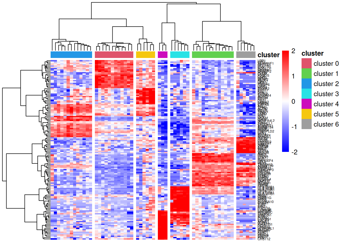
| Version | Author | Date |
|---|---|---|
| 8793f37 | Dave Tang | 2026-02-03 |
In this heatmap:
- Rows represent marker genes, clustered by expression similarity
- Columns represent pseudobulk samples, clustered hierarchically and annotated by cell cluster
- Colours indicate relative expression (blue = low, red = high) after row-wise scaling
- The dendrogram is cut into 7 groups (
cutree_cols=7) to highlight cluster separation
Genes that are good markers should show high expression (red) in their target cluster and low expression (blue) in other clusters.
Alternative parameterisation: Cell means model
The analysis above used a treatment contrast model (also called a reference level model), where the intercept represents the baseline group and other coefficients represent deviations from that baseline. An alternative is the cell means model, which directly estimates the mean expression for each group without an intercept.
The cell means model has several advantages:
- More intuitive contrasts: Each coefficient directly represents a group mean, making it easier to specify comparisons like “cluster 0 vs cluster 1” or “cluster 0 vs average of all others”.
- Symmetric treatment of groups: No group is arbitrarily designated as the “reference” level.
- Clearer interpretation: The design matrix directly shows which group each sample belongs to.
The key difference is in the formula:
- Treatment contrast:
~ cluster + donor(includes intercept) - Cell means:
~ 0 + cluster + donor(no intercept, the0 +removes it)
Despite this different parameterisation, both models fit the same data and produce identical results when equivalent contrasts are specified.
Analysis with a cell means model
Start from the Seurat object and with the same processing steps.
y_cm <- Seurat2PB(so, sample="group", cluster="seurat_clusters")
keep.samples_cm <- y_cm$samples$lib.size > 5e4
y_cm <- y_cm[, keep.samples_cm]
keep.genes_cm <- filterByExpr(y_cm, group=y_cm$samples$cluster)
y_cm <- y_cm[keep.genes_cm, , keep=FALSE]
y_cm <- normLibSizes(y_cm)
Cell means design matrix
The cell means model formula ~ 0 + cluster + donor
creates a design matrix where each cluster has its own column with a 1
indicating membership, rather than having an intercept with deviation
coefficients.
donor_cm <- factor(y_cm$samples$sample)
cluster_cm <- factor(y_cm$samples$cluster)

design_cm <- model.matrix(~ 0 + cluster_cm + donor_cm)
colnames(design_cm) <- gsub("cluster_cm", "cluster", colnames(design_cm))
colnames(design_cm) <- gsub("donor_cm", "", colnames(design_cm))
dim(design_cm)
[1] 59 19The design matrix has 19 columns: 7 (one for each cluster) + 12 (donor coefficients) = 19 parameters. Note that this is the same total number of parameters as before; the intercept has been replaced by an additional cluster coefficient.
head(design_cm) cluster0 cluster1 cluster2 cluster3 cluster4 cluster5 cluster6 N_0021_total
1 1 0 0 0 0 0 0 0
2 0 1 0 0 0 0 0 0
3 0 0 1 0 0 0 0 0
4 0 0 0 1 0 0 0 0
5 0 0 0 0 0 1 0 0
6 0 0 0 0 0 0 1 0
N_0064_total N_0092_total N_0093_total N_0123_total N_0169_total
1 0 0 0 0 0
2 0 0 0 0 0
3 0 0 0 0 0
4 0 0 0 0 0
5 0 0 0 0 0
6 0 0 0 0 0
N_0230.17_total N_0233_total N_0275_total N_0288_total N_0342_total
1 0 0 0 0 0
2 0 0 0 0 0
3 0 0 0 0 0
4 0 0 0 0 0
5 0 0 0 0 0
6 0 0 0 0 0
N_0372_total
1 0
2 0
3 0
4 0
5 0
6 0Instead of an intercept column with 1s everywhere, we now have separate columns for each cluster.
Dispersion and model fitting
y_cm <- estimateDisp(y_cm, design_cm, robust=TRUE)
fit_cm <- glmQLFit(y_cm, design_cm, robust=TRUE)
Constructing equivalent contrasts
Contrasts are more straightforward to specify with the cell means parameterisation. To compare cluster \(k\) against the average of all other clusters, we simply assign:
- Cluster \(k\): weight = 1
- All other clusters: weight = \(-1/6\) (so they average to the comparison group)
- Donor coefficients: weight = 0 (not part of the comparison)
ncls_cm <- nlevels(cluster_cm)
contr_cm <- matrix(0, nrow=ncol(design_cm), ncol=ncls_cm)
rownames(contr_cm) <- colnames(design_cm)
colnames(contr_cm) <- paste0("cluster", levels(cluster_cm))
for(i in 1:ncls_cm) {
  contr_cm[1:ncls_cm, i] <- -1/(ncls_cm - 1)
  contr_cm[i, i] <- 1
}
contr_cm
cluster0 cluster1 cluster2 cluster3 cluster4
cluster0 1.0000000 -0.1666667 -0.1666667 -0.1666667 -0.1666667
cluster1 -0.1666667 1.0000000 -0.1666667 -0.1666667 -0.1666667
cluster2 -0.1666667 -0.1666667 1.0000000 -0.1666667 -0.1666667
cluster3 -0.1666667 -0.1666667 -0.1666667 1.0000000 -0.1666667
cluster4 -0.1666667 -0.1666667 -0.1666667 -0.1666667 1.0000000
cluster5 -0.1666667 -0.1666667 -0.1666667 -0.1666667 -0.1666667
cluster6 -0.1666667 -0.1666667 -0.1666667 -0.1666667 -0.1666667
N_0021_total 0.0000000 0.0000000 0.0000000 0.0000000 0.0000000
N_0064_total 0.0000000 0.0000000 0.0000000 0.0000000 0.0000000
N_0092_total 0.0000000 0.0000000 0.0000000 0.0000000 0.0000000
N_0093_total 0.0000000 0.0000000 0.0000000 0.0000000 0.0000000
N_0123_total 0.0000000 0.0000000 0.0000000 0.0000000 0.0000000
N_0169_total 0.0000000 0.0000000 0.0000000 0.0000000 0.0000000
N_0230.17_total 0.0000000 0.0000000 0.0000000 0.0000000 0.0000000
N_0233_total 0.0000000 0.0000000 0.0000000 0.0000000 0.0000000
N_0275_total 0.0000000 0.0000000 0.0000000 0.0000000 0.0000000
N_0288_total 0.0000000 0.0000000 0.0000000 0.0000000 0.0000000
N_0342_total 0.0000000 0.0000000 0.0000000 0.0000000 0.0000000
N_0372_total 0.0000000 0.0000000 0.0000000 0.0000000 0.0000000
cluster5 cluster6
cluster0 -0.1666667 -0.1666667
cluster1 -0.1666667 -0.1666667
cluster2 -0.1666667 -0.1666667
cluster3 -0.1666667 -0.1666667
cluster4 -0.1666667 -0.1666667
cluster5 1.0000000 -0.1666667
cluster6 -0.1666667 1.0000000
N_0021_total 0.0000000 0.0000000
N_0064_total 0.0000000 0.0000000
N_0092_total 0.0000000 0.0000000
N_0093_total 0.0000000 0.0000000
N_0123_total 0.0000000 0.0000000
N_0169_total 0.0000000 0.0000000
N_0230.17_total 0.0000000 0.0000000
N_0233_total 0.0000000 0.0000000
N_0275_total 0.0000000 0.0000000
N_0288_total 0.0000000 0.0000000
N_0342_total 0.0000000 0.0000000
N_0372_total 0.0000000 0.0000000Each column clearly shows that the tested cluster gets weight 1 and all other clusters get weight \(-1/6\), and donor effects are ignored (weight 0).
Differential expression testing with cell means model
qlf_cm <- list()
for(i in 1:ncls_cm){
  qlf_cm[[i]] <- glmQLFTest(fit_cm, contrast=contr_cm[,i])
  qlf_cm[[i]]$comparison <- paste0("cluster", levels(cluster_cm)[i], "_vs_others")
}
Comparing results: Treatment contrast vs Cell means
Verify that both parameterisations produce identical results by comparing the top DE genes for cluster 0 vs others.
top_tc <- topTags(qlf[[1]], n=10)$table
top_cm <- topTags(qlf_cm[[1]], n=10)$table
identical(rownames(top_tc), rownames(top_cm))
[1] TRUECompare the statistical values.
comparison_df <- data.frame(
  Gene = rownames(top_tc),
  logFC_treatment = round(top_tc$logFC, 6),
  logFC_cellmeans = round(top_cm$logFC, 6),
  FDR_treatment = signif(top_tc$FDR, 6),
  FDR_cellmeans = signif(top_cm$FDR, 6)
)
comparison_df
Gene logFC_treatment logFC_cellmeans FDR_treatment FDR_cellmeans
1 FBLN1 5.983506 5.983508 1.82272e-35 1.82288e-35
2 OGN 5.726554 5.726555 6.58667e-33 6.58728e-33
3 IGFBP6 5.374590 5.374589 2.61963e-31 2.61986e-31
4 DPT 5.893382 5.893384 1.45814e-30 1.45824e-30
5 CFD 4.978584 4.978585 1.32221e-29 1.32229e-29
6 SERPINF1 5.169235 5.169235 1.77120e-29 1.77131e-29
7 MFAP4 4.611371 4.611371 1.99956e-29 1.99972e-29
8 CRABP2 3.948766 3.948766 2.12703e-29 2.12721e-29
9 CLMP 5.951695 5.951696 3.39351e-29 3.39374e-29
10 MMP2 5.377426 5.377427 3.39351e-29 3.39374e-29Compare all logFC values.
all_tc <- qlf[[1]]$table
all_cm <- qlf_cm[[1]]$table

# Ensure same gene order
all_cm <- all_cm[rownames(all_tc), ]

# Check correlation and maximum difference
cat("Correlation of logFC values:", cor(all_tc$logFC, all_cm$logFC), "\n")
Correlation of logFC values: 1 cat("Maximum absolute difference in logFC:", max(abs(all_tc$logFC - all_cm$logFC)), "\n")Maximum absolute difference in logFC: 0.0001427852 cat("Maximum absolute difference in PValue:", max(abs(all_tc$PValue - all_cm$PValue)), "\n")Maximum absolute difference in PValue: 0.0002470824 The results are identical (within numerical precision), confirming that both parameterisations are mathematically equivalent. The choice between them is a matter of convenience and interpretability:
- Treatment contrasts are the R default and work well when you have a natural reference group.
- Cell means models make it easier to specify arbitrary contrasts and may be more intuitive for complex comparisons.
Summary of DE genes comparison
dt_cm <- lapply(lapply(qlf_cm, decideTests), summary)
dt_cm.all <- do.call("cbind", dt_cm)

cat("Treatment contrast model:\n")
Treatment contrast model:print(dt.all) cluster0_vs_others cluster1_vs_others cluster2_vs_others
Down 1478 790 1453
NotSig 3980 4852 4276
Up 2409 2225 2138
cluster3_vs_others cluster4_vs_others cluster5_vs_others
Down 1588 1605 249
NotSig 4408 4942 6573
Up 1871 1320 1045
cluster6_vs_others
Down 1410
NotSig 4880
Up 1577cat("\nCell means model:\n")
Cell means model:print(dt_cm.all) cluster0_vs_others cluster1_vs_others cluster2_vs_others
Down 1478 790 1453
NotSig 3980 4852 4276
Up 2409 2225 2138
cluster3_vs_others cluster4_vs_others cluster5_vs_others
Down 1588 1605 249
NotSig 4408 4942 6573
Up 1871 1320 1045
cluster6_vs_others
Down 1410
NotSig 4880
Up 1577cat("\nDifference (should be all zeros):\n")
Difference (should be all zeros):print(dt.all - dt_cm.all) cluster0_vs_others cluster1_vs_others cluster2_vs_others
Down 0 0 0
NotSig 0 0 0
Up 0 0 0
cluster3_vs_others cluster4_vs_others cluster5_vs_others
Down 0 0 0
NotSig 0 0 0
Up 0 0 0
cluster6_vs_others
Down 0
NotSig 0
Up 0The identical number of DE genes in each category confirms that both approaches yield the same biological conclusions.
Session info
sessionInfo()R version 4.5.0 (2025-04-11)
Platform: x86_64-pc-linux-gnu
Running under: Ubuntu 24.04.3 LTS
Matrix products: default
BLAS: /usr/lib/x86_64-linux-gnu/openblas-pthread/libblas.so.3
LAPACK: /usr/lib/x86_64-linux-gnu/openblas-pthread/libopenblasp-r0.3.26.so; LAPACK version 3.12.0
locale:
[1] LC_CTYPE=en_US.UTF-8 LC_NUMERIC=C
[3] LC_TIME=en_US.UTF-8 LC_COLLATE=en_US.UTF-8
[5] LC_MONETARY=en_US.UTF-8 LC_MESSAGES=en_US.UTF-8
[7] LC_PAPER=en_US.UTF-8 LC_NAME=C
[9] LC_ADDRESS=C LC_TELEPHONE=C
[11] LC_MEASUREMENT=en_US.UTF-8 LC_IDENTIFICATION=C
time zone: Etc/UTC
tzcode source: system (glibc)
attached base packages:
[1] stats graphics grDevices utils datasets methods base
other attached packages:
[1] pheatmap_1.0.13 Seurat_5.3.0 SeuratObject_5.1.0 sp_2.2-0
[5] edgeR_4.6.3 limma_3.64.3 lubridate_1.9.4 forcats_1.0.0
[9] stringr_1.5.1 dplyr_1.1.4 purrr_1.0.4 readr_2.1.5
[13] tidyr_1.3.1 tibble_3.3.0 ggplot2_3.5.2 tidyverse_2.0.0
[17] workflowr_1.7.1
loaded via a namespace (and not attached):
[1] RColorBrewer_1.1-3 rstudioapi_0.17.1 jsonlite_2.0.0
[4] magrittr_2.0.3 spatstat.utils_3.1-5 farver_2.1.2
[7] rmarkdown_2.29 fs_1.6.6 vctrs_0.6.5
[10] ROCR_1.0-11 spatstat.explore_3.5-2 htmltools_0.5.8.1
[13] sass_0.4.10 sctransform_0.4.2 parallelly_1.45.0
[16] KernSmooth_2.23-26 bslib_0.9.0 htmlwidgets_1.6.4
[19] ica_1.0-3 plyr_1.8.9 plotly_4.11.0
[22] zoo_1.8-14 cachem_1.1.0 whisker_0.4.1
[25] igraph_2.1.4 mime_0.13 lifecycle_1.0.4
[28] pkgconfig_2.0.3 Matrix_1.7-3 R6_2.6.1
[31] fastmap_1.2.0 fitdistrplus_1.2-4 future_1.58.0
[34] shiny_1.11.1 digest_0.6.37 colorspace_2.1-1
[37] patchwork_1.3.0 ps_1.9.1 rprojroot_2.0.4
[40] tensor_1.5.1 RSpectra_0.16-2 irlba_2.3.5.1
[43] progressr_0.15.1 spatstat.sparse_3.1-0 timechange_0.3.0
[46] httr_1.4.7 polyclip_1.10-7 abind_1.4-8
[49] compiler_4.5.0 withr_3.0.2 fastDummies_1.7.5
[52] MASS_7.3-65 tools_4.5.0 lmtest_0.9-40
[55] httpuv_1.6.16 future.apply_1.20.0 goftest_1.2-3
[58] glue_1.8.0 callr_3.7.6 nlme_3.1-168
[61] promises_1.3.3 grid_4.5.0 Rtsne_0.17
[64] getPass_0.2-4 cluster_2.1.8.1 reshape2_1.4.4
[67] generics_0.1.4 gtable_0.3.6 spatstat.data_3.1-6
[70] tzdb_0.5.0 data.table_1.17.4 hms_1.1.3
[73] spatstat.geom_3.5-0 RcppAnnoy_0.0.22 ggrepel_0.9.6
[76] RANN_2.6.2 pillar_1.10.2 spam_2.11-1
[79] RcppHNSW_0.6.0 later_1.4.2 splines_4.5.0
[82] lattice_0.22-6 deldir_2.0-4 survival_3.8-3
[85] tidyselect_1.2.1 locfit_1.5-9.12 miniUI_0.1.2
[88] pbapply_1.7-4 knitr_1.50 git2r_0.36.2
[91] gridExtra_2.3 scattermore_1.2 xfun_0.52
[94] statmod_1.5.0 matrixStats_1.5.0 stringi_1.8.7
[97] lazyeval_0.2.2 yaml_2.3.10 evaluate_1.0.3
[100] codetools_0.2-20 cli_3.6.5 uwot_0.2.3
[103] xtable_1.8-4 reticulate_1.43.0 processx_3.8.6
[106] jquerylib_0.1.4 Rcpp_1.0.14 spatstat.random_3.4-1
[109] globals_0.18.0 png_0.1-8 spatstat.univar_3.1-4
[112] parallel_4.5.0 dotCall64_1.2 listenv_0.9.1
[115] viridisLite_0.4.2 scales_1.4.0 ggridges_0.5.6
[118] rlang_1.1.6 cowplot_1.2.0 Time taken to render notebook.
end_time <- Sys.time()
end_time - start_time
Time difference of 1.019748 mins
sessionInfo()R version 4.5.0 (2025-04-11)
Platform: x86_64-pc-linux-gnu
Running under: Ubuntu 24.04.3 LTS
Matrix products: default
BLAS: /usr/lib/x86_64-linux-gnu/openblas-pthread/libblas.so.3
LAPACK: /usr/lib/x86_64-linux-gnu/openblas-pthread/libopenblasp-r0.3.26.so; LAPACK version 3.12.0
locale:
[1] LC_CTYPE=en_US.UTF-8 LC_NUMERIC=C
[3] LC_TIME=en_US.UTF-8 LC_COLLATE=en_US.UTF-8
[5] LC_MONETARY=en_US.UTF-8 LC_MESSAGES=en_US.UTF-8
[7] LC_PAPER=en_US.UTF-8 LC_NAME=C
[9] LC_ADDRESS=C LC_TELEPHONE=C
[11] LC_MEASUREMENT=en_US.UTF-8 LC_IDENTIFICATION=C
time zone: Etc/UTC
tzcode source: system (glibc)
attached base packages:
[1] stats graphics grDevices utils datasets methods base
other attached packages:
[1] pheatmap_1.0.13 Seurat_5.3.0 SeuratObject_5.1.0 sp_2.2-0
[5] edgeR_4.6.3 limma_3.64.3 lubridate_1.9.4 forcats_1.0.0
[9] stringr_1.5.1 dplyr_1.1.4 purrr_1.0.4 readr_2.1.5
[13] tidyr_1.3.1 tibble_3.3.0 ggplot2_3.5.2 tidyverse_2.0.0
[17] workflowr_1.7.1
loaded via a namespace (and not attached):
[1] RColorBrewer_1.1-3 rstudioapi_0.17.1 jsonlite_2.0.0
[4] magrittr_2.0.3 spatstat.utils_3.1-5 farver_2.1.2
[7] rmarkdown_2.29 fs_1.6.6 vctrs_0.6.5
[10] ROCR_1.0-11 spatstat.explore_3.5-2 htmltools_0.5.8.1
[13] sass_0.4.10 sctransform_0.4.2 parallelly_1.45.0
[16] KernSmooth_2.23-26 bslib_0.9.0 htmlwidgets_1.6.4
[19] ica_1.0-3 plyr_1.8.9 plotly_4.11.0
[22] zoo_1.8-14 cachem_1.1.0 whisker_0.4.1
[25] igraph_2.1.4 mime_0.13 lifecycle_1.0.4
[28] pkgconfig_2.0.3 Matrix_1.7-3 R6_2.6.1
[31] fastmap_1.2.0 fitdistrplus_1.2-4 future_1.58.0
[34] shiny_1.11.1 digest_0.6.37 colorspace_2.1-1
[37] patchwork_1.3.0 ps_1.9.1 rprojroot_2.0.4
[40] tensor_1.5.1 RSpectra_0.16-2 irlba_2.3.5.1
[43] progressr_0.15.1 spatstat.sparse_3.1-0 timechange_0.3.0
[46] httr_1.4.7 polyclip_1.10-7 abind_1.4-8
[49] compiler_4.5.0 withr_3.0.2 fastDummies_1.7.5
[52] MASS_7.3-65 tools_4.5.0 lmtest_0.9-40
[55] httpuv_1.6.16 future.apply_1.20.0 goftest_1.2-3
[58] glue_1.8.0 callr_3.7.6 nlme_3.1-168
[61] promises_1.3.3 grid_4.5.0 Rtsne_0.17
[64] getPass_0.2-4 cluster_2.1.8.1 reshape2_1.4.4
[67] generics_0.1.4 gtable_0.3.6 spatstat.data_3.1-6
[70] tzdb_0.5.0 data.table_1.17.4 hms_1.1.3
[73] spatstat.geom_3.5-0 RcppAnnoy_0.0.22 ggrepel_0.9.6
[76] RANN_2.6.2 pillar_1.10.2 spam_2.11-1
[79] RcppHNSW_0.6.0 later_1.4.2 splines_4.5.0
[82] lattice_0.22-6 deldir_2.0-4 survival_3.8-3
[85] tidyselect_1.2.1 locfit_1.5-9.12 miniUI_0.1.2
[88] pbapply_1.7-4 knitr_1.50 git2r_0.36.2
[91] gridExtra_2.3 scattermore_1.2 xfun_0.52
[94] statmod_1.5.0 matrixStats_1.5.0 stringi_1.8.7
[97] lazyeval_0.2.2 yaml_2.3.10 evaluate_1.0.3
[100] codetools_0.2-20 cli_3.6.5 uwot_0.2.3
[103] xtable_1.8-4 reticulate_1.43.0 processx_3.8.6
[106] jquerylib_0.1.4 Rcpp_1.0.14 spatstat.random_3.4-1
[109] globals_0.18.0 png_0.1-8 spatstat.univar_3.1-4
[112] parallel_4.5.0 dotCall64_1.2 listenv_0.9.1
[115] viridisLite_0.4.2 scales_1.4.0 ggridges_0.5.6
[118] rlang_1.1.6 cowplot_1.2.0