Methods Comparison
Last updated: 2024-07-06
Checks: 7 0
Knit directory: MATHPOP/
This reproducible R Markdown analysis was created with workflowr (version 1.7.1). The Checks tab describes the reproducibility checks that were applied when the results were created. The Past versions tab lists the development history.
Great! Since the R Markdown file has been committed to the Git repository, you know the exact version of the code that produced these results.
Great job! The global environment was empty. Objects defined in the global environment can affect the analysis in your R Markdown file in unknown ways. For reproduciblity it’s best to always run the code in an empty environment.
The command set.seed(20240702) was run prior to running
the code in the R Markdown file. Setting a seed ensures that any results
that rely on randomness, e.g. subsampling or permutations, are
reproducible.
Great job! Recording the operating system, R version, and package versions is critical for reproducibility.
Nice! There were no cached chunks for this analysis, so you can be confident that you successfully produced the results during this run.
Great job! Using relative paths to the files within your workflowr project makes it easier to run your code on other machines.
Great! You are using Git for version control. Tracking code development and connecting the code version to the results is critical for reproducibility.
The results in this page were generated with repository version eda1cf3. See the Past versions tab to see a history of the changes made to the R Markdown and HTML files.
Note that you need to be careful to ensure that all relevant files for
the analysis have been committed to Git prior to generating the results
(you can use wflow_publish or
wflow_git_commit). workflowr only checks the R Markdown
file, but you know if there are other scripts or data files that it
depends on. Below is the status of the Git repository when the results
were generated:
Ignored files:
    Ignored:    .DS_Store
    Ignored:    analysis/.DS_Store
    Ignored:    data/.DS_Store
    Ignored:    data/GC_prob/.DS_Store
    Ignored:    data/point_source_data/.DS_Store
    Ignored:    data/prob_GC_data/.DS_Store
    Ignored:    data/sim/.DS_Store
    Ignored:    data/v10acs/.DS_Store
    Ignored:    data/v10wfc3/.DS_Store
    Ignored:    data/v11acs/.DS_Store
    Ignored:    data/v11wfc3/.DS_Store
    Ignored:    data/v12acs/.DS_Store
    Ignored:    data/v12wfc3/.DS_Store
    Ignored:    data/v13acs/.DS_Store
    Ignored:    data/v13wfc3/.DS_Store
    Ignored:    data/v14acs/.DS_Store
    Ignored:    data/v14wfc3/.DS_Store
    Ignored:    data/v15acs/.DS_Store
    Ignored:    data/v15wfc3/.DS_Store
    Ignored:    data/v6acs/.DS_Store
    Ignored:    data/v6wfc3/.DS_Store
    Ignored:    data/v7acs/.DS_Store
    Ignored:    data/v8acs/.DS_Store
    Ignored:    data/v9acs/.DS_Store
    Ignored:    data/v9wfc3/.DS_Store

Untracked files:
    Untracked:  GC_prob-tikzDictionary
    Untracked:  analysis/GC_prob-tikzDictionary
    Untracked:  analysis/data_process-tikzDictionary
    Untracked:  analysis/method_compare-tikzDictionary
    Untracked:  analysis/posterior-tikzDictionary
    Untracked:  analysis/vignette-tikzDictionary
    Untracked:  data_process-tikzDictionary
    Untracked:  method_compare-tikzDictionary
    Untracked:  posterior-tikzDictionary
    Untracked:  vignette-tikzDictionary
Note that any generated files, e.g. HTML, png, CSS, etc., are not included in this status report because it is ok for generated content to have uncommitted changes.
These are the previous versions of the repository in which changes were
made to the R Markdown (analysis/method_compare.Rmd) and
HTML (docs/method_compare.html) files. If you’ve configured
a remote Git repository (see ?wflow_git_remote), click on
the hyperlinks in the table below to view the files as they were in that
past version.
| File | Version | Author | Date | Message |
|---|---|---|---|---|
| html | 0a9d403 | david.li | 2024-07-05 | Build site. |
| html | 388826c | david.li | 2024-07-05 | Build site. |
| Rmd | 2913187 | david.li | 2024-07-05 | wflow_publish(c("analysis/_site.yml", "analysis/method_compare.Rmd")) |
Introduction
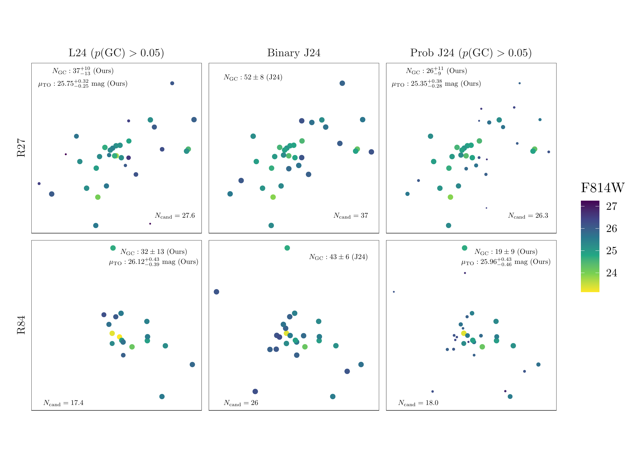
This vignettes contains the analysis and code that compares the results obtained from MATHPOP and those from the standard method, specifically for the UDGs — R27 and R84, as these two UDGs have the largest discrepancy between the two methods. We also reproduces Figure 5 in the original Li et al. (2024) paper.
Data For R27 and R84
R27 is in the field V10-WFC3 and R84 is in the field V7-ACS. We first read in the GC data for R27 from both DOLPHOT and SExtractor in below:
library(tidyverse)
library(sf)
library(sp)
library(raster)
library(parallel)
library(Rcpp)
library(RcppArmadillo)
library(posterior)
library(coda)
library(loo)
library(xtable)
library(priorsense)
library(ggpubr)
library(wesanderson)
library(reshape2)
library(tikzDevice)

sourceCpp('code/cpp_help_func.cpp')
source('code/fit_mod_MCMC.R')

# DOLPHOT V10WFC3
V10WFC <- read_csv('data/prob_GC_data/v10wfc3_pGC.csv')
# SExtractor V10WFC3
V10WFC_J <- read_csv('data/prob_GC_data/V10WFC3_pGC_Jans.csv')

# transform pixel coordinates to pyhsical
V10WFC <- as.data.frame(V10WFC)
V10WFC[,c('x','y')] <- 62*V10WFC[,c('x','y')]/4400
V10WFC_J <- as.data.frame(V10WFC_J)
V10WFC_J[,c('x','y')] <- 62*V10WFC_J[,c('x','y')]/4400

# locations of UDGs in V10WFC3
c <- 62*rbind(c(808, 744), c(1930, 2653), c(2695, 2132))/4400
Next, generate cutout data for R27:
# cutout GC data (within 7.5 kpc radius) for R27 from DOLPHOT
R27_dat_harris <- filter(V10WFC, (x - c[1, 1])^2 + (y - c[1,2])^2 < 7.5^2)
R27_dat_harris$p <- rowMeans(R27_dat_harris[,8:507])
R27_dat_harris <- R27_dat_harris %>%
  filter(p > 0.05) %>%
  dplyr::select(x, y, M, C, p) %>%
  mutate(DATA = 'L24 ($p(\\mathrm{GC}) > 0.05$)')

# cutout probabilistic GC data (within 7.5 kpc radius) for R27 from SExtractor
R27_dat_Jans <- filter(V10WFC_J, (x - c[1, 1])^2 + (y - c[1,2])^2 < 7.5^2)
R27_dat_Jans$p <- rowMeans(R27_dat_Jans[,8:507])
R27_dat_Jans <- R27_dat_Jans %>%
  filter(p > 0.05) %>%
  dplyr::select(x, y, M, C, p) %>%
  mutate(DATA = 'Prob J24 ($p(\\mathrm{GC}) > 0.05$)')

# cutout binary GC data (within 7.5 kpc radius) for R27 from SExtractor (J24)
R27_dat_Jans_bin <- filter(V10WFC_J, (x - c[1, 1])^2 + (y - c[1,2])^2 < 7.5^2)
R27_dat_Jans_bin$p <- 1
R27_dat_Jans_bin <- R27_dat_Jans_bin %>%
  filter(p > 0 & M < 26.3 & C > 0.8 & C < 2.4) %>%
  dplyr::select(x, y, M, C, p) %>%
  mutate(DATA = 'Binary J24')

# combine all data sources
R27_dat <- bind_rows(R27_dat_harris, R27_dat_Jans, R27_dat_Jans_bin)

# construct annotation text in the figure
ann_text_R27 <- data.frame(x = c(9, 9, 16.5, 9, 9, 16, 8.5, 16.5), y = c(17, 16, 5.5, 17, 16, 5.5, 16.5, 5.5),
                           lab = c("$N_{\\mathrm{GC}}: 26_{-9}^{+11}$ (Ours)",
                                   '$\\mu_{\\mathrm{TO}}: 25.35_{-0.28}^{+0.38}$ mag (Ours)',
                                   '$N_{\\mathrm{cand}} = 26.3$',
                                   "$N_{\\mathrm{GC}}: 37_{-13}^{+10}$ (Ours)",
                                   '$\\mu_{\\mathrm{TO}}: 25.75_{-0.25}^{+0.32}$ mag (Ours)',
                                   '$N_{\\mathrm{cand}} = 27.6$',
                                   '$N_{\\mathrm{GC}}: 52\\pm 8$ (J24)',
                                   '$N_{\\mathrm{cand}} = 37$'),
                           DATA = c(rep(c('Prob J24 ($p(\\mathrm{GC}) > 0.05$)', 'L24 ($p(\\mathrm{GC}) > 0.05$)'), each = 3), rep('Binary J24', 2)))

R27_dat$DATA <- factor(R27_dat$DATA, levels = c("L24 ($p(\\mathrm{GC}) > 0.05$)", "Binary J24", "Prob J24 ($p(\\mathrm{GC}) > 0.05$)"))
ann_text_R27$DATA <-  factor(ann_text_R27$DATA, levels = c("L24 ($p(\\mathrm{GC}) > 0.05$)", "Binary J24", "Prob J24 ($p(\\mathrm{GC}) > 0.05$)"))
ann_text_R27$ID <- 'R27'

R27_dat$ID <- 'R27'
Now do the same thing for R84:
# grab V7ACS GC data
V7ACS <- read_csv('data/prob_GC_data/v7acs_pGC.csv')
V7ACS_J <- read_csv('data/prob_GC_data/V7ACS_pGC_Jans.csv')

V7ACS <- as.data.frame(V7ACS)
V7ACS[,c('x','y')] <- 76*V7ACS[,c('x','y')]/4300
V7ACS_J <- as.data.frame(V7ACS_J)
V7ACS_J[,c('x','y')] <- 76*V7ACS_J[,c('x','y')]/4300

# UDG locations in V7ACS
c <- 76*rbind(c(661, 2987), c(1756, 752))/4300

# DOLPHOT GC data
R84_dat_harris <- filter(V7ACS, (x - c[1, 1])^2 + (y - c[1,2])^2 < 7.5^2)
R84_dat_harris$p <- rowMeans(R84_dat_harris[,8:507])
R84_dat_harris <- R84_dat_harris %>%
  filter(p > 0.05) %>%
  dplyr::select(x, y, M, C, p) %>%
  mutate(DATA = 'L24 ($p(\\mathrm{GC}) > 0.05$)')

# SExtractor probabilistic GC data
R84_dat_Jans <- filter(V7ACS_J, (x - c[1, 1])^2 + (y - c[1,2])^2 < 7.5^2)
R84_dat_Jans$p <- rowMeans(R84_dat_Jans[,8:507])
R84_dat_Jans <- R84_dat_Jans %>%
  filter(p > 0.05) %>%
  dplyr::select(x, y, M, C, p) %>%
  mutate(DATA = 'Prob J24 ($p(\\mathrm{GC}) > 0.05$)')

# SExtractor binary GC data
R84_dat_Jans_bin <- filter(V7ACS_J, (x - c[1, 1])^2 + (y - c[1,2])^2 < 7.5^2)
R84_dat_Jans_bin$p <- 1
R84_dat_Jans_bin <- R84_dat_Jans_bin %>%
  filter(p > 0 & M < 26.3 & C > 0.8 & C < 2.4) %>%
  dplyr::select(x, y, M, C, p) %>%
  mutate(DATA = 'Binary J24')

#combine all data
R84_dat <- bind_rows(R84_dat_harris, R84_dat_Jans, R84_dat_Jans_bin) %>%
  filter(C > 0.8)

# construct annotation text
ann_text_R84 <- data.frame(x = c(14.7, 14.7, 7.5, 14.4, 14.4, 7.5, 15.5, 7.5), y = c(59.5, 58.7, 47.5, 59.5, 58.7, 47.5, 59.1, 47.5),
                       lab = c("$N_{\\mathrm{GC}}: 19\\pm 9$ (Ours)",
                               '$\\mu_{\\mathrm{TO}}: 25.96_{-0.46}^{+0.43}$ mag (Ours)',
                               '$N_{\\mathrm{cand}} = 18.0$',
                               "$N_{\\mathrm{GC}}: 32\\pm 13$ (Ours)",
                               '$\\mu_{\\mathrm{TO}}: 26.12_{-0.39}^{+0.43}$ mag (Ours)',
                               '$N_{\\mathrm{cand}} = 17.4$',
                               '$N_{\\mathrm{GC}}: 43\\pm 6$ (J24)',
                               '$N_{\\mathrm{cand}} = 26$'),
                       DATA = c(rep(c('Prob J24 ($p(\\mathrm{GC}) > 0.05$)', 'L24 ($p(\\mathrm{GC}) > 0.05$)'), each = 3), rep('Binary J24',2)))

R84_dat$DATA <- factor(R84_dat$DATA, levels = c("L24 ($p(\\mathrm{GC}) > 0.05$)", "Binary J24", "Prob J24 ($p(\\mathrm{GC}) > 0.05$)"))
ann_text_R84$DATA <-  factor(ann_text_R84$DATA, levels = c("L24 ($p(\\mathrm{GC}) > 0.05$)", "Binary J24", "Prob J24 ($p(\\mathrm{GC}) > 0.05$)"))
ann_text_R84$ID <- 'R84'

ann_text <- bind_rows(ann_text_R27, ann_text_R84)

R84_dat$ID <- 'R84'

# combine all things together
LSBG_dat <- bind_rows(R27_dat, R84_dat)
Now we can plot the cutouts of GC candidates from different catalogs:
ggplot(LSBG_dat, aes(x, y)) + geom_point(aes(color = M, size = p*1.5)) + facet_grid(ID~DATA, scales = 'free', switch = 'y') +
  scale_alpha_identity() + scale_size_identity() +
  geom_text(aes(x = x, y = y, label = lab), data = ann_text, size = 2) +
  scale_color_viridis_c(direction = -1, name = 'F814W') +
  theme_bw() +
  theme(axis.title=element_blank(),
        axis.text=element_blank(),
        axis.ticks=element_blank(),
        strip.background = element_blank(),
        panel.grid.minor = element_blank(),
        panel.grid.major = element_blank(),
        legend.justification = "left",
        legend.box.margin = margin(l = 0.1, unit = "cm"),
        aspect.ratio = 1) +
  guides(fill = guide_legend(title.position = "top", title.hjust = 0.5))
GC catalogs comparison for R27 and R84. (See Figure 5 in the original Li et al. (2024) paper for more details)
| Version | Author | Date |
|---|---|---|
| 388826c | david.li | 2024-07-05 |
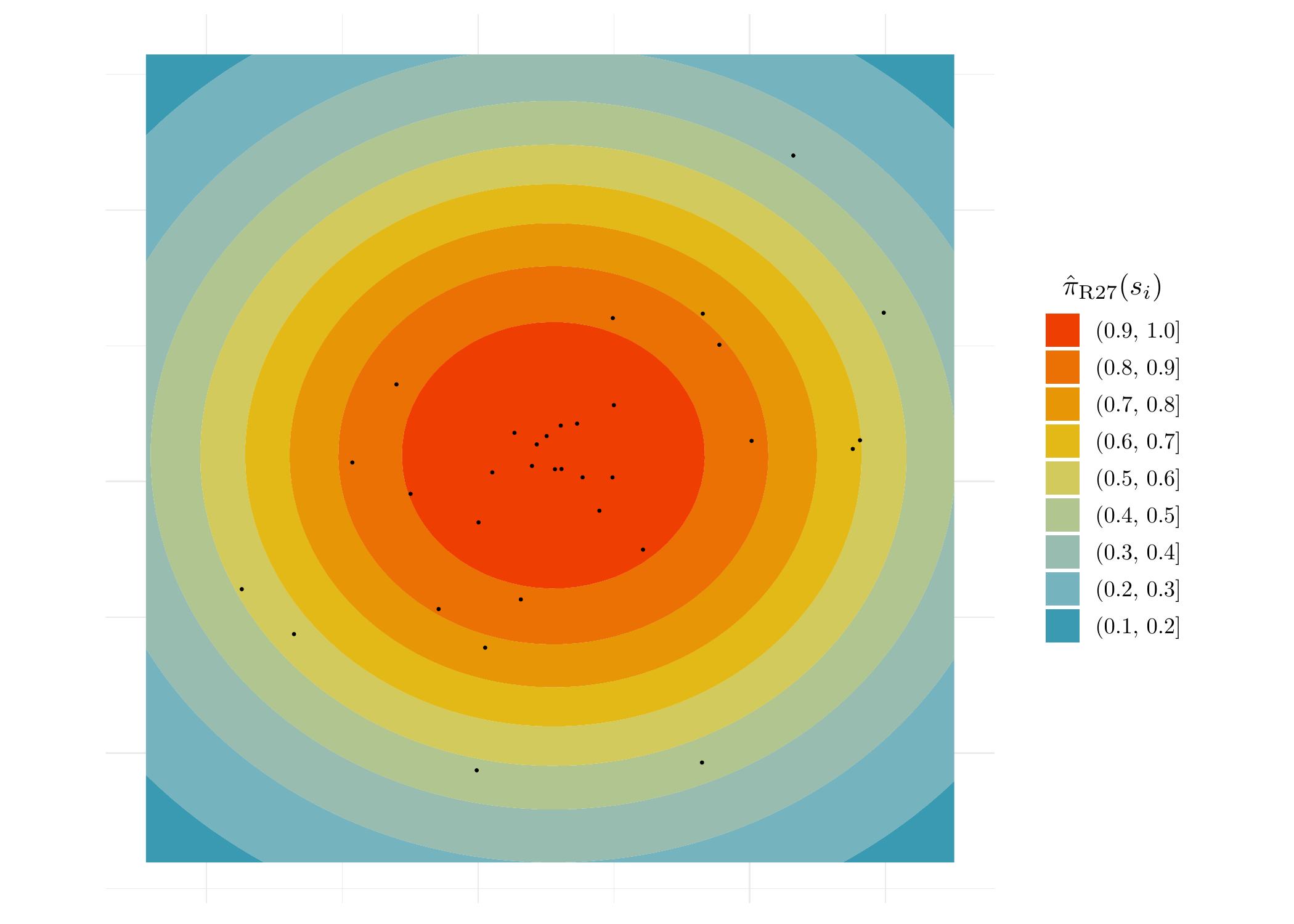
Posterior Probability that a GC belongs to R27
We here show the analysis done to obtain the posterior probability that a GC candidate indeed belongs to R27. Note that the figure produced here was not included in the original paper.
# read in the MCMC results for V10WFC3
res_V10WFC <- readRDS('data/v10wfc3/res_prob_v10wfc3.RDS')

# thin the chain for easier computation
res_V10WFC_thinned <- as.data.frame(res_V10WFC[seq(1, nrow(res_V10WFC), by = 405),])

# locations of UDGs in V10WFC3
c <- 62*rbind(c(808, 744), c(1930, 2653), c(2695, 2132))/4400
# fixed parameters
e <- c(0.88, 1.35, 0.75)
theta <- c(0, -pi/12, 0)

# spatial grid for computing posterior GC membership probabilities
loc <- as.matrix(expand.grid(x = seq(11.38545 - 7.5, 11.38545 + 7.5, by = 0.24), y = seq(10.48364 - 7.5, 10.48364 + 7.5, by = 0.24)))

# function to compute the R27 membership probability for regions around R27
compute_mem_prob <- function(loc, res_prob, e, theta){
  prob <- numeric(nrow(loc))
  loc <- matrix(loc, ncol = 2)
  for (i in 1:nrow(res_prob)) {
    tot <- Sersic_ints(loc, c[1, ], res_prob[i, 'N_R27'], res_prob[i, 'R_R27'],
                       e[1], res_prob[i, 'n_R27'], theta[1]) +
           Sersic_ints(loc, c[2, ], res_prob[i, 'N_W84'], res_prob[i, 'R_W84'],
                       e[2], res_prob[i, 'n_W84'], theta[2]) +
           Sersic_ints(loc, c[3, ], res_prob[i, 'N_W83'], res_prob[i, 'R_W83'],
                       e[3], res_prob[i, 'n_W83'], theta[3]) + res_prob[i, 'b0']

    prob <- prob + Sersic_ints(loc, c[1, ], res_prob[i, 'N_R27'], res_prob[i, 'R_R27'],
                        e[1], res_prob[i, 'n_R27'], theta[1])/tot
  }
  prob <- prob/nrow(res_prob)
  loc <- data.frame(x = loc[,1], y = loc[,2]) %>%
         mutate(p = prob)
  return(loc)
}

# compute the probability
R27_dat_loc <- compute_mem_prob(loc, res_V10WFC_thinned, e, theta)

# plot it
ggplot(R27_dat_loc, aes(x,y)) + geom_contour_filled(aes(z = p)) +
  scale_fill_manual(values = wes_palette("Zissou1", n = 18, type = "continuous")[seq(1,18, by = 2)],
                    name = '$\\hat{\\pi}_{\\mathrm{R27}}(s_i)$') +
  geom_point(data = R27_dat_harris, aes(x, y), size = 0.25) + coord_fixed() +
  theme_minimal() +
  theme(axis.title=element_blank(),
        axis.text=element_blank(),
        axis.ticks=element_blank(),
        strip.background = element_blank(),
        legend.justification = "left",
        legend.box.margin = margin(l = 0.1, unit = "cm")) +
  guides(fill = guide_legend(title.position = "top", title.hjust = 0.5, reverse = TRUE))
Probabilities that a GC candidates belong to R27.
| Version | Author | Date |
|---|---|---|
| 388826c | david.li | 2024-07-05 |
From the above figure, we see that the posterior probabilities for GC candidates in the outer region of R27 are only around \(50\%\). This means that the membership of these GC candidates are highly uncertain, which is one factor that contributes to the big difference between the estimates from MATHPOP and the standard method.
sessionInfo()R version 4.3.2 (2023-10-31)
Platform: aarch64-apple-darwin20 (64-bit)
Running under: macOS Sonoma 14.1.1
Matrix products: default
BLAS: /Library/Frameworks/R.framework/Versions/4.3-arm64/Resources/lib/libRblas.0.dylib
LAPACK: /Library/Frameworks/R.framework/Versions/4.3-arm64/Resources/lib/libRlapack.dylib; LAPACK version 3.11.0
locale:
[1] en_US.UTF-8/en_US.UTF-8/en_US.UTF-8/C/en_US.UTF-8/en_US.UTF-8
time zone: America/Toronto
tzcode source: internal
attached base packages:
[1] parallel stats graphics grDevices utils datasets methods
[8] base
other attached packages:
[1] progress_1.2.2 tikzDevice_0.12.5 reshape2_1.4.4
[4] wesanderson_0.3.7 ggpubr_0.6.0 priorsense_0.0.0.9000
[7] xtable_1.8-4 loo_2.6.0 coda_0.19-4
[10] posterior_1.5.0 RcppArmadillo_0.12.6.6.0 Rcpp_1.0.11
[13] raster_3.6-26 sp_2.1-1 sf_1.0-14
[16] lubridate_1.9.3 forcats_1.0.0 stringr_1.5.1
[19] dplyr_1.1.4 purrr_1.0.2 readr_2.1.4
[22] tidyr_1.3.0 tibble_3.2.1 ggplot2_3.4.4
[25] tidyverse_2.0.0 workflowr_1.7.1
loaded via a namespace (and not attached):
[1] DBI_1.1.3 rlang_1.1.4 magrittr_2.0.3
[4] git2r_0.33.0 matrixStats_1.1.0 e1071_1.7-13
[7] compiler_4.3.2 getPass_0.2-4 png_0.1-8
[10] callr_3.7.3 vctrs_0.6.5 pkgconfig_2.0.3
[13] crayon_1.5.2 fastmap_1.2.0 magick_2.8.3
[16] backports_1.4.1 labeling_0.4.3 utf8_1.2.4
[19] promises_1.2.1 rmarkdown_2.25 tzdb_0.4.0
[22] ps_1.7.5 tinytex_0.48 bit_4.0.5
[25] xfun_0.41 cachem_1.0.8 jsonlite_1.8.7
[28] highr_0.10 later_1.3.1 terra_1.7-55
[31] broom_1.0.5 prettyunits_1.2.0 R6_2.5.1
[34] bslib_0.5.1 stringi_1.8.4 car_3.1-2
[37] jquerylib_0.1.4 assertthat_0.2.1 knitr_1.45
[40] klippy_0.0.0.9500 filehash_2.4-5 httpuv_1.6.12
[43] timechange_0.2.0 tidyselect_1.2.0 rstudioapi_0.15.0
[46] abind_1.4-5 yaml_2.3.7 codetools_0.2-19
[49] processx_3.8.2 qpdf_1.3.3 lattice_0.22-5
[52] plyr_1.8.9 withr_2.5.2 askpass_1.2.0
[55] evaluate_0.23 isoband_0.2.7 units_0.8-4
[58] proxy_0.4-27 pillar_1.9.0 carData_3.0-5
[61] tensorA_0.36.2 whisker_0.4.1 KernSmooth_2.23-22
[64] checkmate_2.3.1 distributional_0.3.2 generics_0.1.3
[67] vroom_1.6.4 rprojroot_2.0.4 hms_1.1.3
[70] munsell_0.5.0 scales_1.3.0 class_7.3-22
[73] glue_1.6.2 tools_4.3.2 ggsignif_0.6.4
[76] pdftools_3.4.0 fs_1.6.3 grid_4.3.2
[79] colorspace_2.1-0 cli_3.6.1 fansi_1.0.6
[82] viridisLite_0.4.2 zipfR_0.6-70 gtable_0.3.4
[85] rstatix_0.7.2 sass_0.4.7 digest_0.6.36
[88] classInt_0.4-10 farver_2.1.1 htmltools_0.5.8.1
[91] lifecycle_1.0.4 httr_1.4.7 bit64_4.0.5