Last updated: 2021-03-21

Checks: 7 0

Knit directory: hesc-epigenomics/

This reproducible R Markdown analysis was created with workflowr (version 1.6.2). The Checks tab describes the reproducibility checks that were applied when the results were created. The Past versions tab lists the development history.


Great! Since the R Markdown file has been committed to the Git repository, you know the exact version of the code that produced these results.

Great job! The global environment was empty. Objects defined in the global environment can affect the analysis in your R Markdown file in unknown ways. For reproduciblity it’s best to always run the code in an empty environment.

The command set.seed(20210202) was run prior to running the code in the R Markdown file. Setting a seed ensures that any results that rely on randomness, e.g. subsampling or permutations, are reproducible.

Great job! Recording the operating system, R version, and package versions is critical for reproducibility.

Nice! There were no cached chunks for this analysis, so you can be confident that you successfully produced the results during this run.

Great job! Using relative paths to the files within your workflowr project makes it easier to run your code on other machines.

Great! You are using Git for version control. Tracking code development and connecting the code version to the results is critical for reproducibility.

The results in this page were generated with repository version 701a84d. See the Past versions tab to see a history of the changes made to the R Markdown and HTML files.

Note that you need to be careful to ensure that all relevant files for the analysis have been committed to Git prior to generating the results (you can use wflow_publish or wflow_git_commit). workflowr only checks the R Markdown file, but you know if there are other scripts or data files that it depends on. Below is the status of the Git repository when the results were generated:


Ignored files:
    Ignored:    .Rhistory
    Ignored:    .Rproj.user/
    Ignored:    analysis/annotations_extended.Rmd
    Ignored:    data/bed/
    Ignored:    data/bw
    Ignored:    data/igv/
    Ignored:    data/meta/
    Ignored:    data/peaks
    Ignored:    data/rnaseq/

Untracked files:
    Untracked:  analysis/global_bins.Rmd
    Untracked:  analysis/histone_marks_vs_expression.Rmd
    Untracked:  output/annotations/

Unstaged changes:
    Modified:   code/deseq_functions.R
    Modified:   data/README.md

Note that any generated files, e.g. HTML, png, CSS, etc., are not included in this status report because it is ok for generated content to have uncommitted changes.


These are the previous versions of the repository in which changes were made to the R Markdown (analysis/annotations.Rmd) and HTML (docs/annotations.html) files. If you’ve configured a remote Git repository (see ?wflow_git_remote), click on the hyperlinks in the table below to view the files as they were in that past version.

File Version Author Date Message
Rmd 701a84d cnluzon 2021-03-21 Annotations cleanup
Rmd ef20c53 cnluzon 2021-03-11 Annotations
html ef20c53 cnluzon 2021-03-11 Annotations

Summary

This notebook shows how the genome annotations relevant for this publication were calculated.

  • Gene annotation: Genes obtained from UCSC hg38.
  • Bivalent genes: Genes from UCSC hg38 overlapping with bivalent peaks from (Court and Arnaud 2017).
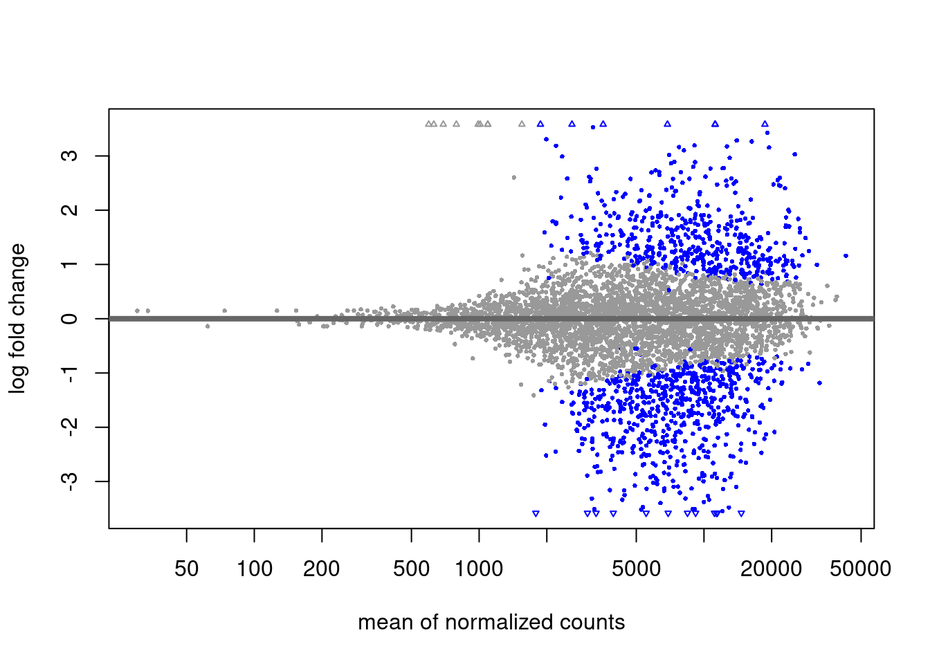
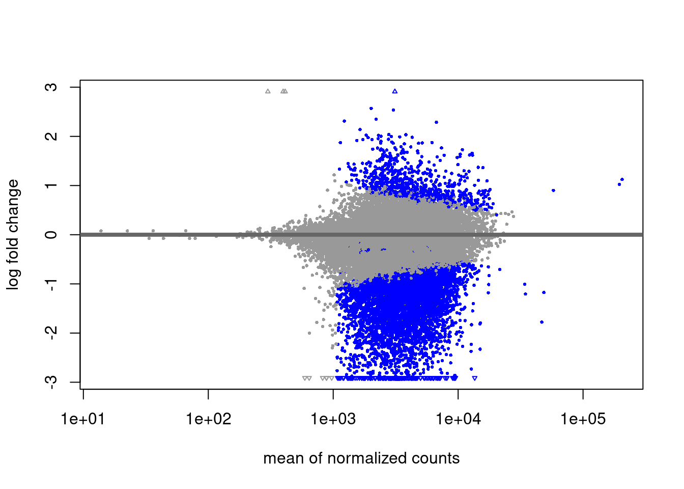
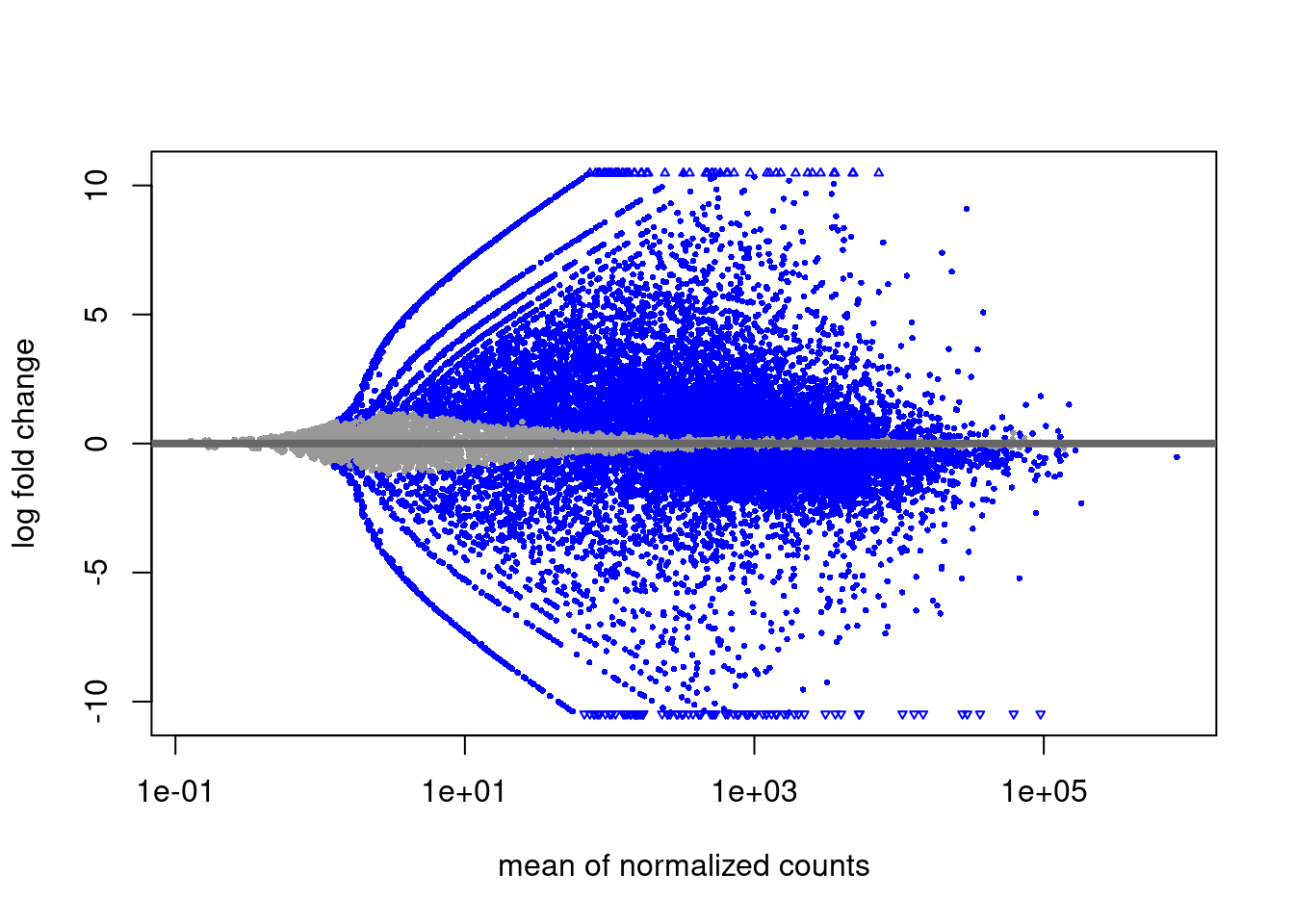
  • Differential TSS per histone mark: H2AUb and H3K4m3 +/- 1500 bp used. H3K27m3: +/- 2500bp used, as this is a broader mark. DESeq2 (Love, Huber, and Anders 2014) was used ad-hoc for our Minute-ChIP data. See deseq_functions.R for more details. Naïve condition was used as reference for enrichment / depletion. Genes were selected if adjusted p value from DESeq2 was lower than 0.05 and absolute value of log2 fold change was > 1. A separate annotation was created for genes selected by this procedure that overlapped with bivalent genes: H2AUb, H3K4m3, H3K27m3.
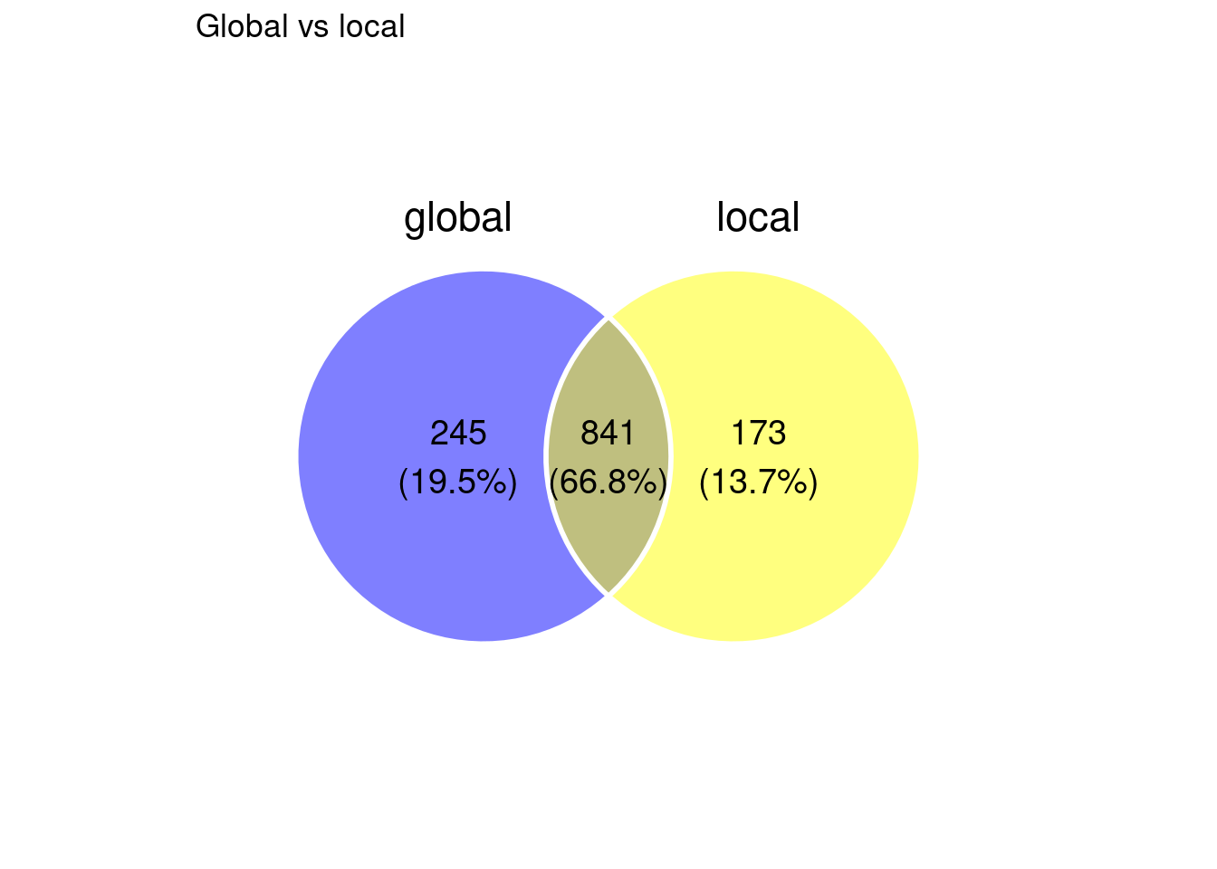
  • Differential 10000 bp bins per histone mark: DESeq2 was used in the same way as differential TSS. Bins were selected by p-value only. These results are cached and / or skipped in this notebook because this is a very memory-demanding step: H2AUb, H3K4m3, H3K27m3.
  • Gene expression groups: Data from (Collier et al. 2017) was used to select top-med-low groups of genes by expression. Genes were pre-filtered by transcript length (> 500) and minimum TPM (0.01) and top, med and low 10% of genes were retained per replicate. Genes were annotated to each of these categories if they appeared in all three replicates within the given range. Downloads: Naïve top, med and low. Primed top, med and low.
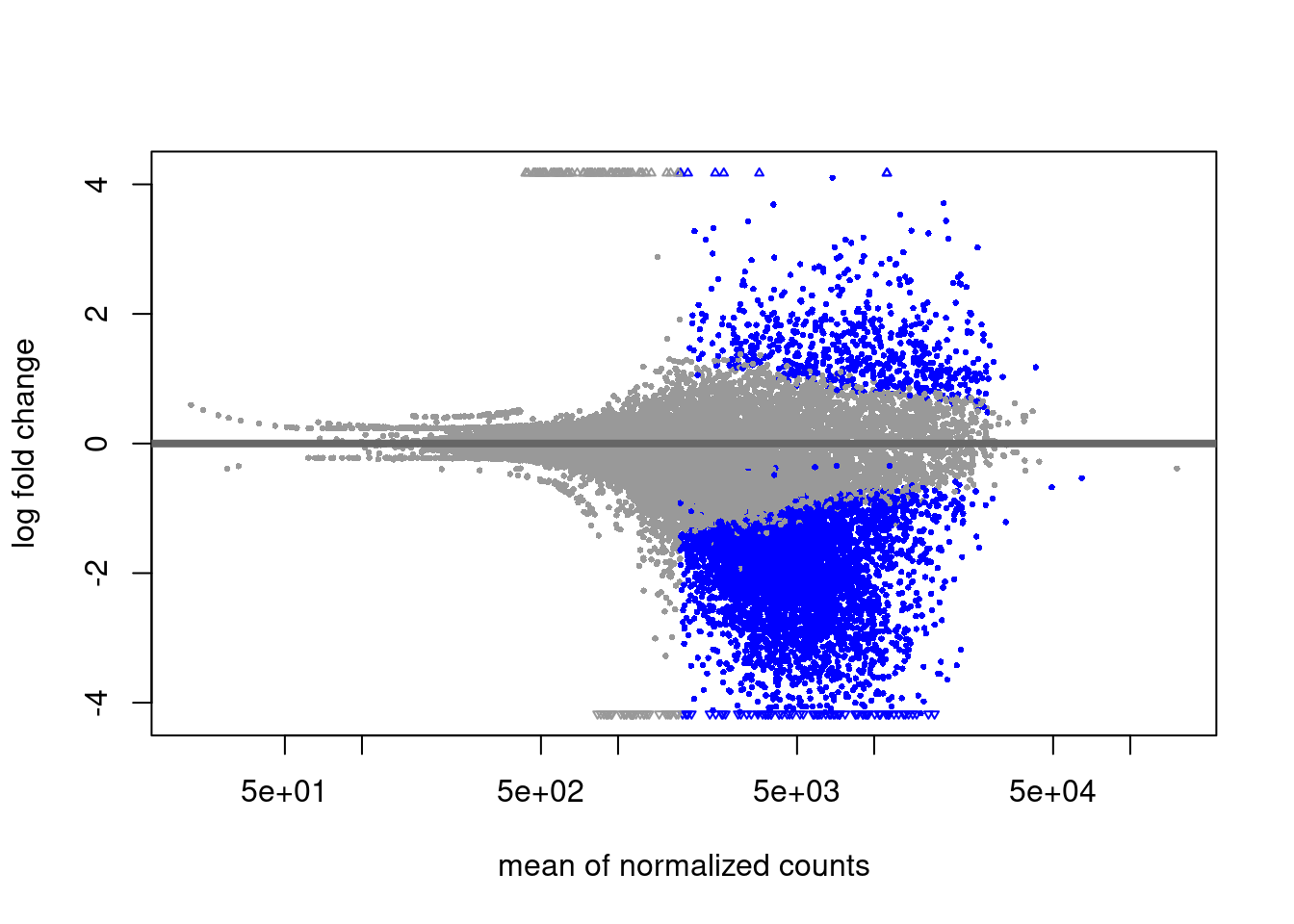
  • Differentially expressed genes: Data from (Collier et al. 2017) was analysed with DESeq2 to obtain Naïve vs. Primed differentially expressed genes. Genes were selected if adjusted p value from DESeq2 was lower than 0.05 and absolute value of log2 fold change was > 1. Downloads: Naïve_up, Naïve_down.
  • Master gene table. All gene-specific annotations above are summarized in a gene table. Each gene along with their locus has a column for each histone mark and also expression data.

Helper functions

#' Select DESeq results by pval and fc cutoff and returns GRanges
#'
#' @param diff_lfc Results dataframe
#' @param loci Corresponding GRanges
#' @param p_cutoff Pvalue cutoff
#' @param fc_cutoff Fold change cutoff
#'
#' @return GRanges with filtered elements
select_signif <- function(diff_lfc, loci, p_cutoff = 0.05, fc_cutoff = 1) {
  diff_lfc <- diff_lfc[!is.na(diff_lfc$padj), ]
  signif_tss <- diff_lfc[diff_lfc$padj <= p_cutoff & abs(diff_lfc$log2FoldChange) > fc_cutoff, ]

  mcols(loci) <- NULL
  signif_gr <- loci[as.numeric(rownames(signif_tss)), ]
  signif_gr$score <- signif_tss$log2FoldChange
  signif_gr
}


#' Intersect 3 gene results by gene name
#'
#' @param glist List of gene results
#' @param field Field used to intersect
#'
#' @return A list of intersecting elements
intersect_genes_3 <- function(glist, field = "gene_id") {
  intersect(intersect(glist[[1]][[field]], 
                      glist[[2]][[field]]),
                      glist[[3]][[field]])
}

#' Subset a named granges by name
#'
#' @param names Names list
#' @param granges GRanges to subset.
#'
#' @return GRanges
select_genes <- function(names, granges) {
  sort(granges[granges$name %in% names, ])
}

#' Export genes that overlap in a set of replicates (3)
#'
#' @param replicates Gene counts results list
#' @param path Output file
export_gene_set <- function(replicates, path) {
  gene_names <- intersect_genes_3(replicates)
  genes_all <- genes_hg38()
  genes_all <- genes_all[, "name"]

  result <- select_genes(gene_names, genes_all)
  export(result, path)
}

#' Select by quantile
#'
#' @param counts Counts table.
#' @param length_cutoff Gene length cutoff.
#' @param value_cutoff Value cutoff
#' @param min_q Minimum quantile to consider
#' @param max_q Maximum quantile to consider
#' @param field Which field to use (default = TPM).
#'
#' @return filtered data.frame
quantile_group <- function(counts, min_q, max_q,
                           value_cutoff = 0,
                           length_cutoff = 500,
                           field = "TPM") {

    counts <- dplyr::filter(counts, .data[[field]] > value_cutoff &
                            length > length_cutoff)
    
    q <- quantile(counts[, field], probs = c(min_q, max_q))
    dplyr::filter(counts, .data[[field]] >= q[1] & .data[[field]] <= q[2])
}

Gene annotation

Gene annotation is obtained from UCSC hg38 annotation.

genes <- genes_hg38()

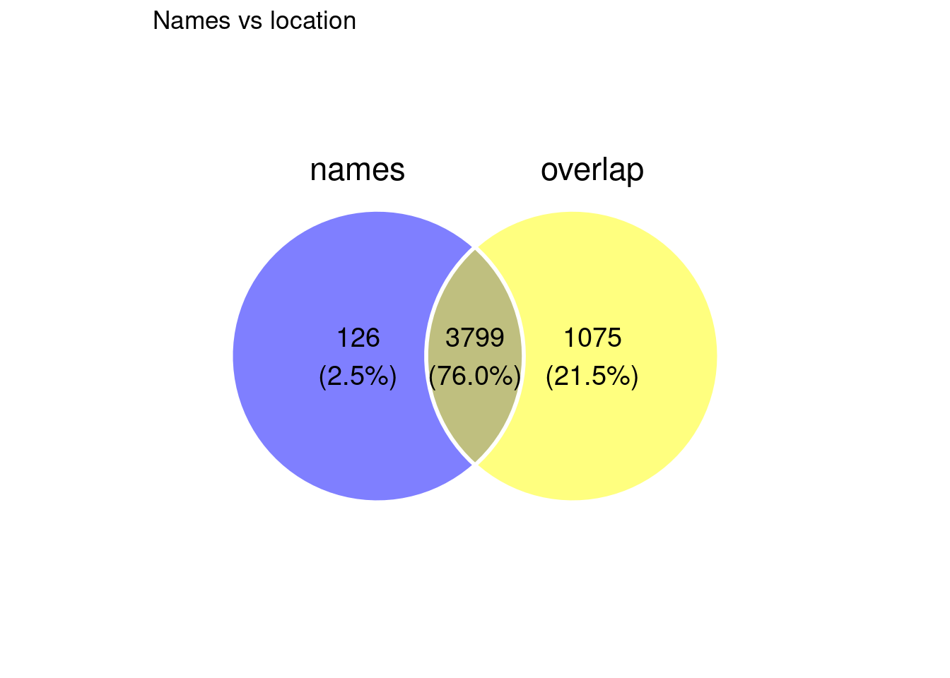
Only genes that have a gene symbol associated to it are kept, leaving a set of 25747.

Download gene annotation.

Bivalent genes by name

Bivalent genes are obtained from UCSC hg38 annotation using as names the ones in (Court and Arnaud 2017) supplementary table.

gene_file <- file.path(params$datadir, "meta/Court_2017_gene_names_uniq.txt")
gene_list <- read.table(gene_file, header=F)
colnames(gene_list) <- c("name")

biv_genes_name <- get_genes_by_name(gene_list$name)

From the list of 5378 gene names from (Court and Arnaud 2017), 3925 unique genomic loci are successfully retrieved.

Download bivalent gene annotation.

Download genes list.

Bivalent genes by overlap

Bivalent genes are obtained from overlap of hg38-liftovered from original (Court and Arnaud 2017) genes with UCSC hg38 annotation.

gene_file <- file.path(params$datadir, "bed/Bivalent_Court2017.hg38.bed")
gene_loci <- import(gene_file)

biv_genes_overlap <- get_genes_by_overlap(gene_loci)

export(biv_genes_overlap, "./data/bed/Kumar_2020/Court_2017_bivalent_genes.bed")

From the list of 5378 gene names from (Court and Arnaud 2017), 4874 unique genomic loci are successfully retrieved.

Download bivalent gene annotation.

Match between both

field_list <- list(names = biv_genes_name$name, overlap = biv_genes_overlap$name)
ggvenn(field_list, fill_alpha = 0.5, text_size = 5, stroke_color = "#ffffff") + 
    ggtitle("Names vs location")

Version Author Date
ef20c53 cnluzon 2021-03-11

Some of the names cases are: either the gene has not been annotated because locus is proximal to annotation but not overlapping it (this may be because of lift over of coordinates), or because the name from UCSC hg38 annotation does not match the name in Court 2017 original annotated gene name.

H3K27m3 differential TSS

bw_cond_1 <-
  list.files(
    file.path(params$datadir, "bw/Kumar_2020"),
    full.names = T,
    pattern = "H3K27m3_H9_Ni_rep[1-3].hg38.scaled.bw"
  )
bw_cond_2 <-
  list.files(
    file.path(params$datadir, "bw/Kumar_2020"),
    full.names = T,
    pattern = "H3K27m3_H9_Pr_rep[1-3].hg38.scaled.bw"
  )

all_hg38_genes <- genes_hg38()
tss <- promoters(all_hg38_genes, upstream = 2500, downstream = 2500)
mcols(tss) <- NULL

c1 <- bw_loci(bw_cond_1, tss)
c2 <- bw_loci(bw_cond_2, tss)

diff <- bw_granges_diff_analysis(c1, c2, "Naive", "Primed", estimate_size_factors = FALSE)

diff_lfc <- lfcShrink(diff, coef="condition_Primed_vs_Naive", type="apeglm")
diff <- results(diff, alpha = params$pval_cutoff)

plotMA(diff_lfc)

Version Author Date
ef20c53 cnluzon 2021-03-11
signif_gr <- select_signif(diff, c1, p_cutoff = params$pval_cutoff)
hits <- findOverlaps(signif_gr, all_hg38_genes)
signif_gr_w_name <- signif_gr
signif_gr_w_name$name <- "None"
signif_gr_w_name[queryHits(hits), ]$name <- all_hg38_genes[subjectHits(hits), ]$name

export(signif_gr_w_name, file.path(params$outgenes, "Kumar_2020_H3K27m3_diff_tss.bed"))

# Select bivalent ones
signif_gr_biv <- subsetByOverlaps(signif_gr_w_name, biv_genes_overlap)
export(signif_gr_biv, file.path(params$outgenes, "Kumar_2020_H3K27m3_diff_bivalent.bed"))

Bivalent

biv_genes <- biv_genes_overlap
tss <- promoters(biv_genes, upstream = 2500, downstream = 2500)
mcols(tss) <- NULL

c1 <- bw_loci(bw_cond_1, tss)
c2 <- bw_loci(bw_cond_2, tss)

diff <- bw_granges_diff_analysis(c1, c2, "Naive", "Primed", estimate_size_factors = FALSE)
diff_lfc <- lfcShrink(diff, coef="condition_Primed_vs_Naive", type="apeglm")
diff <- results(diff, alpha = params$pval_cutoff)
plotMA(diff_lfc)

Version Author Date
ef20c53 cnluzon 2021-03-11
signif_gr <- select_signif(diff, c1, p_cutoff = params$pval_cutoff)

# export(signif_gr, "./data/bed/Kumar_2020_H3K27m3_diff_tss_bivalent.bed")

Compare

global <- import(file.path(params$outgenes, "Kumar_2020_H3K27m3_diff_bivalent.bed"))
local <- subsetByOverlaps(biv_genes_overlap, signif_gr)
field_list <- list(global = global$name, local = local$name)
ggvenn(field_list, fill_alpha = 0.5, text_size = 5, stroke_color = "#ffffff") + 
    ggtitle("Global vs local")

Version Author Date
ef20c53 cnluzon 2021-03-11

H2Aub differential TSS

bw_cond_1 <-
  list.files(
    file.path(params$datadir, "bw/Kumar_2020"),
    full.names = T,
    pattern = "H2Aub_H9_Ni_rep[1-3].hg38.scaled.bw"
  )
bw_cond_2 <-
  list.files(
    file.path(params$datadir, "bw/Kumar_2020"),
    full.names = T,
    pattern = "H2Aub_H9_Pr_rep[1-3].hg38.scaled.bw"
  )

all_hg38_genes <- genes_hg38()
tss <- promoters(all_hg38_genes, upstream = 1500, downstream = 1500)
mcols(tss) <- NULL

c1 <- bw_loci(bw_cond_1, tss)
c2 <- bw_loci(bw_cond_2, tss)

diff <- bw_granges_diff_analysis(c1, c2, "Naive", "Primed", estimate_size_factors = FALSE)
diff_lfc <- lfcShrink(diff, coef="condition_Primed_vs_Naive", type="apeglm")

diff <- results(diff, alpha = params$pval_cutoff)
plotMA(diff_lfc)

Version Author Date
ef20c53 cnluzon 2021-03-11
signif_gr <- select_signif(diff, c1, p_cutoff = params$pval_cutoff)

hits <- findOverlaps(signif_gr, all_hg38_genes)
signif_gr_w_name <- signif_gr
signif_gr_w_name$name <- "None"
signif_gr_w_name[queryHits(hits), ]$name <- all_hg38_genes[subjectHits(hits), ]$name
export(signif_gr_w_name, file.path(params$outgenes, "Kumar_2020_H2Aub_diff_tss.bed"))

# Select bivalent ones
signif_gr_biv <- subsetByOverlaps(signif_gr_w_name, biv_genes_overlap)
export(signif_gr_biv, file.path(params$outgenes, "Kumar_2020_H2Aub_diff_bivalent.bed"))

H3K4m3 differential TSS

bw_cond_1 <-
  list.files(
    file.path(params$datadir, "bw/Kumar_2020"),
    full.names = T,
    pattern = "H3K4m3_H9_Ni_rep[1-3].hg38.scaled.bw"
  )
bw_cond_2 <-
  list.files(
    file.path(params$datadir, "bw/Kumar_2020"),
    full.names = T,
    pattern = "H3K4m3_H9_Pr_rep[1-3].hg38.scaled.bw"
  )

all_hg38_genes <- genes_hg38()
tss <- promoters(all_hg38_genes, upstream = 1500, downstream = 1500)
mcols(tss) <- NULL

c1 <- bw_loci(bw_cond_1, tss)
c2 <- bw_loci(bw_cond_2, tss)

diff <- bw_granges_diff_analysis(c1, c2, "Naive", "Primed", estimate_size_factors = FALSE)

diff_lfc <- lfcShrink(diff, coef="condition_Primed_vs_Naive", type="apeglm")
diff <- results(diff, alpha = params$pval_cutoff)

plotMA(diff_lfc)

Version Author Date
ef20c53 cnluzon 2021-03-11
signif_gr <- select_signif(diff, c1, p_cutoff = params$pval_cutoff)

hits <- findOverlaps(signif_gr, all_hg38_genes)
signif_gr_w_name <- signif_gr
signif_gr_w_name$name <- "None"
signif_gr_w_name[queryHits(hits), ]$name <- all_hg38_genes[subjectHits(hits), ]$name
export(signif_gr_w_name, file.path(params$outgenes, "Kumar_2020_H3K4m3_diff_tss.bed"))

# Select bivalent ones
signif_gr_biv <- subsetByOverlaps(signif_gr_w_name, biv_genes_overlap)
export(signif_gr_biv, file.path(params$outgenes, "Kumar_2020_H3K4m3_diff_bivalent.bed"))

Genome-wide differential test annotation

H3K27m3 differential 10000bp bins

bw_cond_1 <-
  list.files(
    file.path(params$datadir, "bw/Kumar_2020"),
    full.names = T,
    pattern = "H3K27m3_H9_Ni_rep[1-3].hg38.scaled.bw"
  )
bw_cond_2 <-
  list.files(
    file.path(params$datadir, "bw/Kumar_2020"),
    full.names = T,
    pattern = "H3K27m3_H9_Pr_rep[1-3].hg38.scaled.bw"
  )

bs <- params$bin_size
c1 <- bw_bins(bw_cond_1, bin_size = bs, genome = "hg38")
c2 <- bw_bins(bw_cond_2, bin_size = bs, genome = "hg38")

diff <- bw_granges_diff_analysis(c1, c2, "Naive", "Primed", estimate_size_factors = FALSE)
diff <- results(diff, alpha = params$pval_cutoff)

mcols(c1) <- NULL
c1$logfc <- diff$log2FoldChange
c1$padj <- diff$padj

p_cutoff <- params$pval_cutoff
c1$score <- 0
c1 <- c1[!is.na(c1$padj), ]
c1[c1$padj <= p_cutoff & c1$logfc > 0, ]$score <- 1 
c1[c1$padj <= p_cutoff & c1$logfc < 0, ]$score <- -1
c1 <- c1[c1$padj <= p_cutoff]
export(c1, file.path(params$outbins, "Kumar_2020_H3K27m3_signif_ni_05.bed"))

Warning: The above code chunk cached its results, but it won’t be re-run if previous chunks it depends on are updated. If you need to use caching, it is highly recommended to also set knitr::opts_chunk$set(autodep = TRUE) at the top of the file (in a chunk that is not cached). Alternatively, you can customize the option dependson for each individual chunk that is cached. Using either autodep or dependson will remove this warning. See the knitr cache options for more details.

H3K4m3 differential 10000bp bins

bw_cond_1 <-
  list.files(
    file.path(params$datadir, "bw/Kumar_2020"),
    full.names = T,
    pattern = "H3K4m3_H9_Ni_rep[1-3].hg38.scaled.bw"
  )
bw_cond_2 <-
  list.files(
    file.path(params$datadir, "bw/Kumar_2020"),
    full.names = T,
    pattern = "H3K4m3_H9_Pr_rep[1-3].hg38.scaled.bw"
  )

bs <-  params$bin_size
c1 <- bw_bins(bw_cond_1, bin_size = bs, genome = "hg38")
c2 <- bw_bins(bw_cond_2, bin_size = bs, genome = "hg38")

diff <- bw_granges_diff_analysis(c2, c1, "Primed", "Naive", estimate_size_factors = FALSE)
diff <- results(diff, alpha = params$pval_cutoff)

mcols(c1) <- NULL
c1$logfc <- diff$log2FoldChange
c1$padj <- diff$padj

p_cutoff <- params$pval_cutoff
c1$score <- 0
c1 <- c1[!is.na(c1$padj), ]
c1[c1$padj <= p_cutoff & c1$logfc > 0, ]$score <- 1 
c1[c1$padj <= p_cutoff & c1$logfc < 0, ]$score <- -1
c1 <- c1[c1$padj <= p_cutoff]
export(c1, file.path(params$outbins, "Kumar_2020_H3K4m3_signif_ni_05.bed"))

Warning: The above code chunk cached its results, but it won’t be re-run if previous chunks it depends on are updated. If you need to use caching, it is highly recommended to also set knitr::opts_chunk$set(autodep = TRUE) at the top of the file (in a chunk that is not cached). Alternatively, you can customize the option dependson for each individual chunk that is cached. Using either autodep or dependson will remove this warning. See the knitr cache options for more details.

H2AUb differential 10000bp bins

bw_cond_1 <-
  list.files(
    file.path(params$datadir, "bw/Kumar_2020"),
    full.names = T,
    pattern = "H2Aub_H9_Ni_rep[1-3].hg38.scaled.bw"
  )
bw_cond_2 <-
  list.files(
    file.path(params$datadir, "bw/Kumar_2020"),
    full.names = T,
    pattern = "H2Aub_H9_Pr_rep[1-3].hg38.scaled.bw"
  )

bs <- params$bin_size

c1 <- bw_bins(bw_cond_1, bin_size = bs, genome = "hg38")
c2 <- bw_bins(bw_cond_2, bin_size = bs, genome = "hg38")

diff <- bw_granges_diff_analysis(c1, c2, "Naive", "Primed", estimate_size_factors = FALSE)
diff <- results(diff, alpha = params$pval_cutoff)

mcols(c1) <- NULL
c1$logfc <- diff$log2FoldChange
c1$padj <- diff$padj

p_cutoff <- params$pval_cutoff
c1$score <- 0
c1 <- c1[!is.na(c1$padj), ]
c1[c1$padj <= p_cutoff & c1$logfc > 0, ]$score <- 1 
c1[c1$padj <= p_cutoff & c1$logfc < 0, ]$score <- -1
c1 <- c1[c1$padj <= p_cutoff]
export(c1, file.path(params$outbins,"Kumar_2020_H2AUb_signif_ni_05.bed"))

Warning: The above code chunk cached its results, but it won’t be re-run if previous chunks it depends on are updated. If you need to use caching, it is highly recommended to also set knitr::opts_chunk$set(autodep = TRUE) at the top of the file (in a chunk that is not cached). Alternatively, you can customize the option dependson for each individual chunk that is cached. Using either autodep or dependson will remove this warning. See the knitr cache options for more details.

Gene expression levels on Naïve and Primed hESC cells

Data: Used public data from (Collier et al. 2017): H9 embryonic stem cells in Naïve and Primed state, three biological replicates.

Sample info
dataset_id gsm_id description filename run_id input layout experiment
26 Collier_2017 GSM2449055 hESC_H9_naive_1 hESC_H9_naive_1 SRR5151102 - single RNA-seq
27 Collier_2017 GSM2449056 hESC_H9_naive_2 hESC_H9_naive_2 SRR5151103 - single RNA-seq
28 Collier_2017 GSM2449057 hESC_H9_naive_3 hESC_H9_naive_3 SRR5151104 - single RNA-seq
29 Collier_2017 GSM2449058 hESC_H9_primed_1 hESC_H9_primed_1 SRR5151105 - single RNA-seq
30 Collier_2017 GSM2449059 hESC_H9_primed_2 hESC_H9_primed_2 SRR5151106 - single RNA-seq
31 Collier_2017 GSM2449060 hESC_H9_primed_3 hESC_H9_primed_3 SRR5151107 - single RNA-seq

Primary analysis

RNA-seq data was analysed by a standard RNA-seq pipeline v2.0, available on nf-core (Ewels et al. 2019) with mostly default settings. For more information about the specific steps involved in this analysis, refer to the repository documentation: https://nf-co.re/rnaseq/2.0, using the option --aligner star_rsem.

Reference genome used was hg38, downloaded from illumina iGenomes:

http://igenomes.illumina.com.s3-website-us-east-1.amazonaws.com/Homo_sapiens/UCSC/hg38/Homo_sapiens_UCSC_hg38.tar.gz

Gene expression groups

rsem_files <- list(
  naive = list.files(params$rnaseqdir,
                     pattern = "Naive.*genes.results", full.names = T),
  primed = list.files(params$rnaseqdir,
                      pattern = "Primed.*genes.results", full.names = T)
)

counts_naive <- lapply(rsem_files$naive,
                       read.csv,
                       header = T,
                       sep = "\t")

counts_primed <- lapply(rsem_files$primed,
                        read.csv,
                        header = T,
                        sep = "\t")

# Size of the quantile group
size = 0.1

min_qs <- c(0, 0.5 - (size/2), 1-size)
max_qs <- c(0+size, 0.5 + (size/2), 1)

quantile_low <- purrr::partial(
  quantile_group,
  min_q = min_qs[1],
  max_q = max_qs[1],
  length_cutoff = params$length_cutoff,
  value_cutoff = params$value_cutoff,
  field = params$deciding_stat
)

quantile_med <- purrr::partial(
  quantile_group,
  min_q = min_qs[2],
  max_q = max_qs[2],
  length_cutoff = params$length_cutoff,
  value_cutoff = params$value_cutoff,
  field = params$deciding_stat
)

quantile_high <- purrr::partial(
  quantile_group,
  min_q = min_qs[3],
  max_q = max_qs[3],
  length_cutoff = params$length_cutoff,
  value_cutoff = params$value_cutoff,
  field = params$deciding_stat
)


naive_top <- map(counts_naive, quantile_high)
naive_med <- map(counts_naive, quantile_med)
naive_low <- map(counts_naive, quantile_low)

primed_top <- map(counts_primed, quantile_high)
primed_med <- map(counts_primed, quantile_med)
primed_low <- map(counts_primed, quantile_low)

export_gene_set(naive_top, file.path("./data/bed/Collier_2017", "Collier_2017_Naive_top.bed"))
export_gene_set(naive_med, file.path("./data/bed/Collier_2017", "Collier_2017_Naive_med.bed"))
export_gene_set(naive_low, file.path("./data/bed/Collier_2017", "Collier_2017_Naive_low.bed"))

export_gene_set(primed_top, file.path("./data/bed/Collier_2017", "Collier_2017_Primed_top.bed"))
export_gene_set(primed_med, file.path("./data/bed/Collier_2017", "Collier_2017_Primed_med.bed"))
export_gene_set(primed_low, file.path("./data/bed/Collier_2017", "Collier_2017_Primed_low.bed"))

Differentially expressed genes

Aggregate annotation

Here I build a table where each Gene is annotated with flags:

  • Bivalent: Yes or no.
  • H3K27m3: Up, down or same (TSS). Up means Naïve is significantly higher than primed.
  • H3K4me3: Up, down or same (TSS).
  • H2AUb: Up, down or same (TSS).
  • Expression: Up, down or same. Again, up means Naïve is higher than primed.
  • X-chromosome: Yes or no.
annotate_up_and_down <- function(df, gr, field) {
  df[[field]] <- 0
  names_up <- gr[gr$score > 0, ]$name
  df[names_up, field] <- 1
  names_down <- gr[gr$score < 0, ]$name
  df[names_down, field] <- -1
  df
}

genes_all <- genes_hg38()

annotations <- c("./data/bed/Kumar_2020/Court_2017_bivalent_genes.bed",
                 "./data/bed/Kumar_2020/gene_stats/Kumar_2020_H3K27m3_diff_tss.bed",
                 "./data/bed/Kumar_2020/gene_stats/Kumar_2020_H3K4m3_diff_tss.bed",
                 "./data/bed/Kumar_2020/gene_stats/Kumar_2020_H2Aub_diff_tss.bed",
                 "./data/bed/Collier_2017/Collier_2017_Naive_up_05_logfc1.bed",
                 "./data/bed/Collier_2017/Collier_2017_Naive_down_05_logfc1.bed")

gr_annot <- lapply(annotations, import)

df <- data.frame(genes_all)
rownames(df) <- df$name

df$bivalent <- 0
df[gr_annot[[1]]$name, "bivalent"] <- 1

df <- annotate_up_and_down(df, gr_annot[[2]], "H3K27m3")
df <- annotate_up_and_down(df, gr_annot[[3]], "H3K4m3")
df <- annotate_up_and_down(df, gr_annot[[4]], "H2Aub")

df$expression <- 0
df[gr_annot[[5]]$name, "expression"] <- 1
df[gr_annot[[6]]$name, "expression"] <- -1

df$chrX <- 0
df[df$seqnames == "chrX", "chrX"] <- 1

write.table(df, "./data/bed/Kumar_2020_gene_annotation_table.tsv", row.names = F, sep = "\t", quote = F)

# write.table(df, "./data/bed/Kumar_2020_gene_annotation_table_verbose.tsv", row.names = F, sep = "\t", quote = F)
Collier, Amanda J, Sarita P Panula, John Paul Schell, Peter Chovanec, Alvaro Plaza Reyes, Sophie Petropoulos, Anne E Corcoran, et al. 2017. “Comprehensive Cell Surface Protein Profiling Identifies Specific Markers of Human Naive and Primed Pluripotent States.” Cell Stem Cell 20 (6): 874–90.
Court, Franck, and Philippe Arnaud. 2017. “An Annotated List of Bivalent Chromatin Regions in Human ES Cells: A New Tool for Cancer Epigenetic Research.” Oncotarget 8 (3): 4110.
Ewels, Philip A, Alexander Peltzer, Sven Fillinger, Johannes Alneberg, Harshil Patel, Andreas Wilm, Maxime Ulysse Garcia, Paolo Di Tommaso, and Sven Nahnsen. 2019. “Nf-Core: Community Curated Bioinformatics Pipelines.” BioRxiv, 610741.
Love, Michael I, Wolfgang Huber, and Simon Anders. 2014. “Moderated Estimation of Fold Change and Dispersion for RNA-Seq Data with DESeq2.” Genome Biology 15 (12): 1–21.

sessionInfo()
R version 4.0.4 (2021-02-15)
Platform: x86_64-pc-linux-gnu (64-bit)
Running under: Ubuntu 20.04.2 LTS

Matrix products: default
BLAS:   /usr/lib/x86_64-linux-gnu/openblas-pthread/libblas.so.3
LAPACK: /usr/lib/x86_64-linux-gnu/openblas-pthread/liblapack.so.3

locale:
 [1] LC_CTYPE=en_US.UTF-8       LC_NUMERIC=C              
 [3] LC_TIME=sv_SE.UTF-8        LC_COLLATE=en_US.UTF-8    
 [5] LC_MONETARY=sv_SE.UTF-8    LC_MESSAGES=en_US.UTF-8   
 [7] LC_PAPER=sv_SE.UTF-8       LC_NAME=C                 
 [9] LC_ADDRESS=C               LC_TELEPHONE=C            
[11] LC_MEASUREMENT=sv_SE.UTF-8 LC_IDENTIFICATION=C       

attached base packages:
 [1] stats4    parallel  grid      stats     graphics  grDevices utils    
 [8] datasets  methods   base     

other attached packages:
 [1] DESeq2_1.30.0                           
 [2] SummarizedExperiment_1.20.0             
 [3] MatrixGenerics_1.2.0                    
 [4] matrixStats_0.58.0                      
 [5] tidyr_1.1.2                             
 [6] cowplot_1.1.1                           
 [7] xfun_0.21                               
 [8] purrr_0.3.4                             
 [9] rtracklayer_1.50.0                      
[10] org.Hs.eg.db_3.11.4                     
[11] TxDb.Hsapiens.UCSC.hg38.knownGene_3.10.0
[12] GenomicFeatures_1.40.1                  
[13] AnnotationDbi_1.52.0                    
[14] Biobase_2.50.0                          
[15] GenomicRanges_1.42.0                    
[16] GenomeInfoDb_1.26.2                     
[17] IRanges_2.24.1                          
[18] S4Vectors_0.28.1                        
[19] BiocGenerics_0.36.0                     
[20] ggvenn_0.1.8                            
[21] dplyr_1.0.4                             
[22] knitr_1.31                              
[23] ggplot2_3.3.3                           
[24] wigglescout_0.12.8                      
[25] workflowr_1.6.2                         

loaded via a namespace (and not attached):
 [1] colorspace_2.0-0         ellipsis_0.3.1           rprojroot_2.0.2         
 [4] XVector_0.30.0           fs_1.5.0                 listenv_0.8.0           
 [7] furrr_0.2.2              farver_2.0.3             bit64_4.0.5             
[10] mvtnorm_1.1-1            apeglm_1.10.0            xml2_1.3.2              
[13] codetools_0.2-18         splines_4.0.4            cachem_1.0.4            
[16] geneplotter_1.68.0       Rsamtools_2.6.0          annotate_1.68.0         
[19] dbplyr_2.1.0             compiler_4.0.4           httr_1.4.2              
[22] assertthat_0.2.1         Matrix_1.3-2             fastmap_1.1.0           
[25] later_1.1.0.1            htmltools_0.5.1.1        prettyunits_1.1.1       
[28] tools_4.0.4              coda_0.19-4              gtable_0.3.0            
[31] glue_1.4.2               GenomeInfoDbData_1.2.4   reshape2_1.4.4          
[34] rappdirs_0.3.3           Rcpp_1.0.6               bbmle_1.0.23.1          
[37] vctrs_0.3.6              Biostrings_2.58.0        stringr_1.4.0           
[40] globals_0.14.0           lifecycle_1.0.0          XML_3.99-0.5            
[43] future_1.21.0            MASS_7.3-53.1            zlibbioc_1.36.0         
[46] scales_1.1.1             hms_1.0.0                promises_1.2.0.1        
[49] RColorBrewer_1.1-2       yaml_2.2.1               curl_4.3                
[52] memoise_2.0.0            emdbook_1.3.12           bdsmatrix_1.3-4         
[55] biomaRt_2.44.4           stringi_1.5.3            RSQLite_2.2.3           
[58] highr_0.8                genefilter_1.72.0        BiocParallel_1.24.1     
[61] rlang_0.4.10             pkgconfig_2.0.3          bitops_1.0-6            
[64] evaluate_0.14            lattice_0.20-41          GenomicAlignments_1.26.0
[67] labeling_0.4.2           bit_4.0.4                tidyselect_1.1.0        
[70] parallelly_1.23.0        plyr_1.8.6               magrittr_2.0.1          
[73] R6_2.5.0                 generics_0.1.0           DelayedArray_0.16.0     
[76] DBI_1.1.1                pillar_1.4.7             whisker_0.4             
[79] withr_2.4.1              survival_3.2-7           RCurl_1.98-1.2          
[82] tibble_3.0.6             crayon_1.4.1             BiocFileCache_1.12.1    
[85] rmarkdown_2.6            progress_1.2.2           locfit_1.5-9.4          
[88] blob_1.2.1               git2r_0.28.0             digest_0.6.27           
[91] xtable_1.8-4             numDeriv_2016.8-1.1      httpuv_1.5.5            
[94] openssl_1.4.3            munsell_0.5.0            askpass_1.1