Histone marks at gene groups per expression level
Carmen Navarro
2021-02-07
Last updated: 2021-02-07
Checks: 7 0
Knit directory: hesc-epigenomics/
This reproducible R Markdown analysis was created with workflowr (version 1.6.2). The Checks tab describes the reproducibility checks that were applied when the results were created. The Past versions tab lists the development history.
Great! Since the R Markdown file has been committed to the Git repository, you know the exact version of the code that produced these results.
Great job! The global environment was empty. Objects defined in the global environment can affect the analysis in your R Markdown file in unknown ways. For reproduciblity it’s best to always run the code in an empty environment.
The command set.seed(20210202) was run prior to running the code in the R Markdown file. Setting a seed ensures that any results that rely on randomness, e.g. subsampling or permutations, are reproducible.
Great job! Recording the operating system, R version, and package versions is critical for reproducibility.
Nice! There were no cached chunks for this analysis, so you can be confident that you successfully produced the results during this run.
Great job! Using relative paths to the files within your workflowr project makes it easier to run your code on other machines.
Great! You are using Git for version control. Tracking code development and connecting the code version to the results is critical for reproducibility.
The results in this page were generated with repository version f903045. See the Past versions tab to see a history of the changes made to the R Markdown and HTML files.
Note that you need to be careful to ensure that all relevant files for the analysis have been committed to Git prior to generating the results (you can use wflow_publish or wflow_git_commit). workflowr only checks the R Markdown file, but you know if there are other scripts or data files that it depends on. Below is the status of the Git repository when the results were generated:
Ignored files:
    Ignored:    .Rhistory
    Ignored:    .Rproj.user/
    Ignored:    data/bed/
    Ignored:    data/bw
    Ignored:    data/meta/
    Ignored:    data/peaks
    Ignored:    data/rnaseq/

Unstaged changes:
    Modified:   analysis/index.Rmd
Note that any generated files, e.g. HTML, png, CSS, etc., are not included in this status report because it is ok for generated content to have uncommitted changes.
These are the previous versions of the repository in which changes were made to the R Markdown (analysis/gene_expression_groups.Rmd) and HTML (docs/gene_expression_groups.html) files. If you’ve configured a remote Git repository (see ?wflow_git_remote), click on the hyperlinks in the table below to view the files as they were in that past version.
| File | Version | Author | Date | Message |
|---|---|---|---|---|
| Rmd | f903045 | cnluzon | 2021-02-07 | Histone marks per gene group report |
Summary
Here we look at our histone marks in gene groups separated by expression levels (high-med-low) per cell type. These groups were calculated using RNA-seq data from [@collier2017]. For more details, see corresponding analysis report.
Helper functions
colors_list <- c("Naive_EZH2i"="#5F9EA0",
                 "Naive_Untreated"="#278b8b",
                 "Primed_EZH2i"="#f47770",
                 "Primed_Untreated"="#f44b34")

style_info <- read.table(params$styles, header = T, sep = "\t")
rownames(style_info) <- style_info$bw

# Clean unnecesary labels in a grid
remove_extra_captions <- function(plot_list) {
  for (i in 2:length(plot_list)) {
    plot_list[[i]] <- plot_list[[i]] + theme(legend.position = "none") + ggtitle("")
  }
  plot_list
}

set_global_y_axis <- function(plot_list, limits) {
  for (i in 1:length(plot_list)) {
    plot_list[[i]] <- plot_list[[i]] + ylim(limits)
  }
  plot_list
}
H3K27m3
Highly expressed genes
bedfiles <- list.files(params$genesdir, full.names = T, pattern = "top")
bwfiles <- list.files(params$bwdir, full.names = T)

bwinput <- bwfiles[grepl("IN.*pooled", bwfiles)]
bwsignal <- bwfiles[grepl("H3K27m3.*pooled.hg38.scaled", bwfiles)]

colors <- as.character(style_info[basename(c(bwsignal, bwinput)), "color_cond"])
labels <- style_info[basename(c(bwsignal, bwinput)), "label"]

up <- 10000
dw <- 10000
bs <- 500
md <- "stretch"
global_lims <- c(0, 1.5)

this_plot <- partial(plot_bw_profile, bwfiles = c(bwsignal, bwinput),
                     bin_size = bs,
                     mode = md,
                     upstream = up,
                     downstream = dw,
                     colors = colors,
                     labels = labels)

plots <- purrr::map(bedfiles, this_plot)
plots[[1]] <- plots[[1]] + ylim(global_lims) + theme(legend.position = "none") + ggtitle("H3K27m3 @Top genes")
plots[[2]] <- plots[[2]] + ylim(global_lims) + ylab("") + ggtitle("")

plot_grid(plotlist=plots, nrow=1)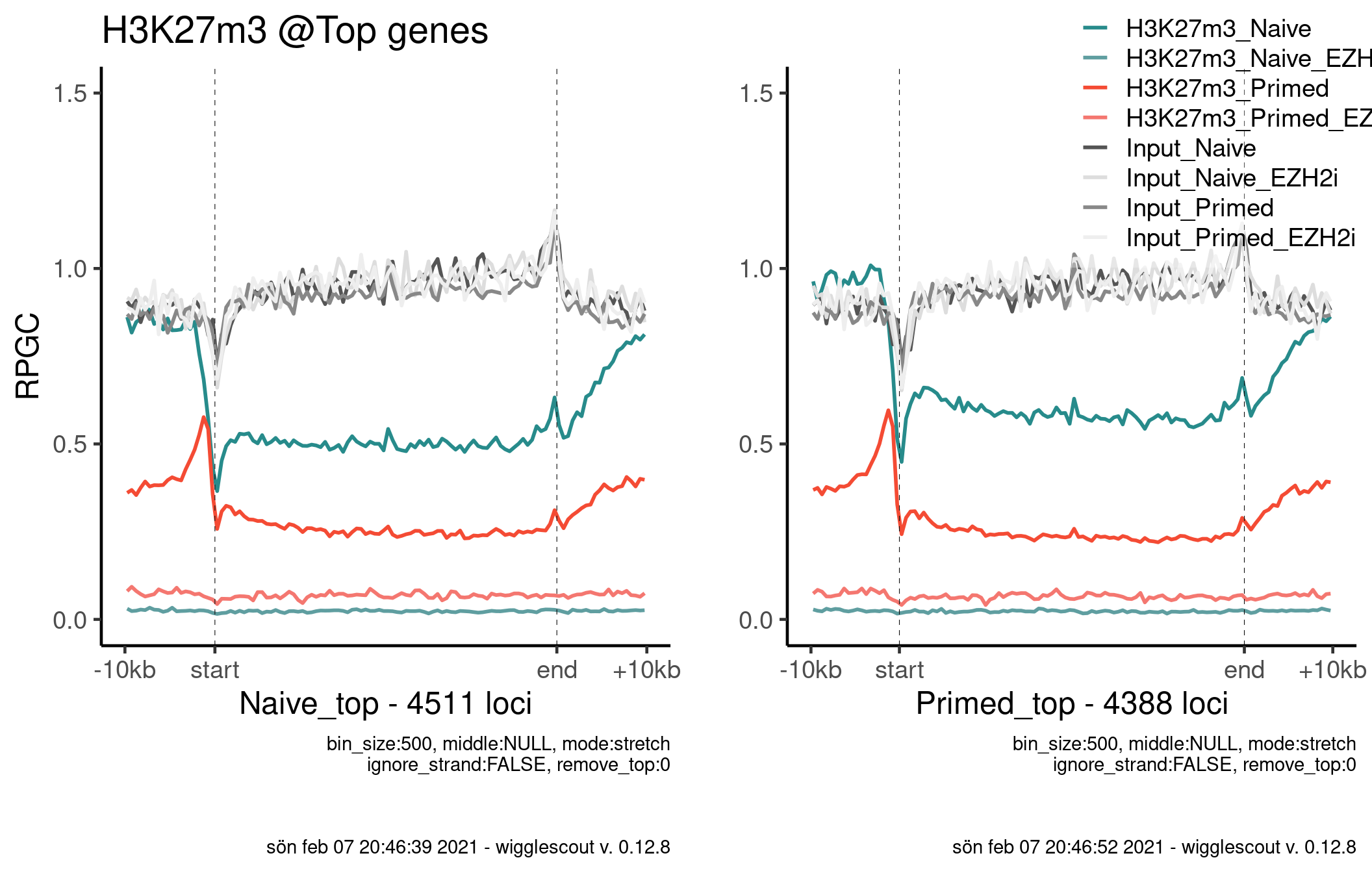
Norm to input
colors <- as.character(style_info[basename(bwsignal), "color_cond"])
labels <- style_info[basename(bwsignal), "label"]

global_lims <- c(0, 1.2)

this_plot <- partial(plot_bw_profile, bwfiles = bwsignal, bg_bwfiles = bwinput,
                     bin_size = bs,
                     mode = md,
                     upstream = up,
                     downstream = dw,
                     colors = colors,
                     labels = labels)

plots <- purrr::map(bedfiles, this_plot)
plots[[1]] <- plots[[1]] + ylim(global_lims) + theme(legend.position = "none") + ggtitle("H3K27m3 @Top genes")
plots[[2]] <- plots[[2]] + ylim(global_lims) + ylab("") + ggtitle("")

plot_grid(plotlist=plots, nrow=1)
As shown in the previous report, there is some overlap between these groups of genes:
naive_top <- import(bedfiles[[1]])
primed_top <- import(bedfiles[[2]])

field_list <- list(naive=naive_top$name,
                   primed=primed_top$name)

ggvenn(field_list, fill_color = c(colors_list[["Naive_Untreated"]], colors_list[["Primed_Untreated"]]), fill_alpha = 0.5, text_size = 5, stroke_color = "#ffffff") +
    ggtitle("Naive vs primed top expressed genes")
Naive-only vs primed-only
naive_only_top <- setdiff(naive_top, primed_top)
primed_only_top <- setdiff(primed_top, naive_top)
both <- intersect(naive_top, primed_top)

colors <- as.character(style_info[basename(c(bwsignal, bwinput)), "color_cond"])
labels <- style_info[basename(c(bwsignal, bwinput)), "label"]

global_lims <- c(0, 2)

this_plot <- partial(plot_bw_profile, bwfiles = c(bwsignal, bwinput),
                     bin_size = bs,
                     mode = md,
                     upstream = up,
                     downstream = dw,
                     colors = colors,
                     labels = labels)


plots <- purrr::map(list(naive_only_top, primed_only_top, both), this_plot)
plots[[1]] <- plots[[1]] + ylim(global_lims) + theme(legend.position = "none") + ggtitle("Naive-only")
plots[[2]] <- plots[[2]] + ylim(global_lims) + ylab("") + theme(legend.position = "none") + ggtitle("Primed-only")
plots[[3]] <- plots[[3]] + ylim(global_lims) + ylab("") + ggtitle("Both")

plot_grid(plotlist=plots, ncol=2)
Norm to input
colors <- as.character(style_info[basename(bwsignal), "color_cond"])
labels <- style_info[basename(bwsignal), "label"]

global_lims <- c(0, 2)

this_plot <- partial(plot_bw_profile, bwfiles = bwsignal, bg_bwfiles = bwinput,
                     bin_size = bs,
                     mode = md,
                     upstream = up,
                     downstream = dw,
                     colors = colors,
                     labels = labels)


plots <- purrr::map(list(naive_only_top, primed_only_top, both), this_plot)
plots[[1]] <- plots[[1]] + ylim(global_lims) + theme(legend.position = "none") + ggtitle("Naive-only")
plots[[2]] <- plots[[2]] + ylim(global_lims) + ylab("") + theme(legend.position = "none") + ggtitle("Primed-only")
plots[[3]] <- plots[[3]] + ylim(global_lims) + ylab("") + ggtitle("Both")

plot_grid(plotlist=plots, ncol=2)
High-med-low expressed genes
bedfiles_top <- list.files(params$genesdir, full.names = T, pattern = "_top")
bedfiles_med <- list.files(params$genesdir, full.names = T, pattern = "_med")
bedfiles_bottom <- list.files(params$genesdir, full.names = T, pattern = "_bottom")

# Ensures proper order
bedfiles <- c(bedfiles_top, bedfiles_med, bedfiles_bottom)
bwsignal <- bwfiles[grepl("H3K27m3.*pooled.hg38.scaled", bwfiles)]

colors <- as.character(style_info[basename(c(bwsignal, bwinput)), "color_cond"])
labels <- style_info[basename(c(bwsignal, bwinput)), "label"]

up <- 10000
dw <- 10000
bs <- 500
md <- "stretch"
global_lims <- c(0, 2.5)

this_plot <- partial(plot_bw_profile, bwfiles = c(bwsignal, bwinput),
                     bin_size = bs,
                     mode = md,
                     upstream = up,
                     downstream = dw,
                     colors = colors,
                     labels = labels,
                     verbose = FALSE) # Plot gets too crowded

plots <- purrr::map(bedfiles, this_plot)

plots <- remove_extra_captions(plots)
plots <- set_global_y_axis(plots, global_lims)

plots[[1]] <- plots[[1]] + ggtitle("H3K27m3 per gene class: Naive")
plots[[2]] <- plots[[2]] + ggtitle("- Primed" )

plot_grid(plotlist=plots, nrow=3)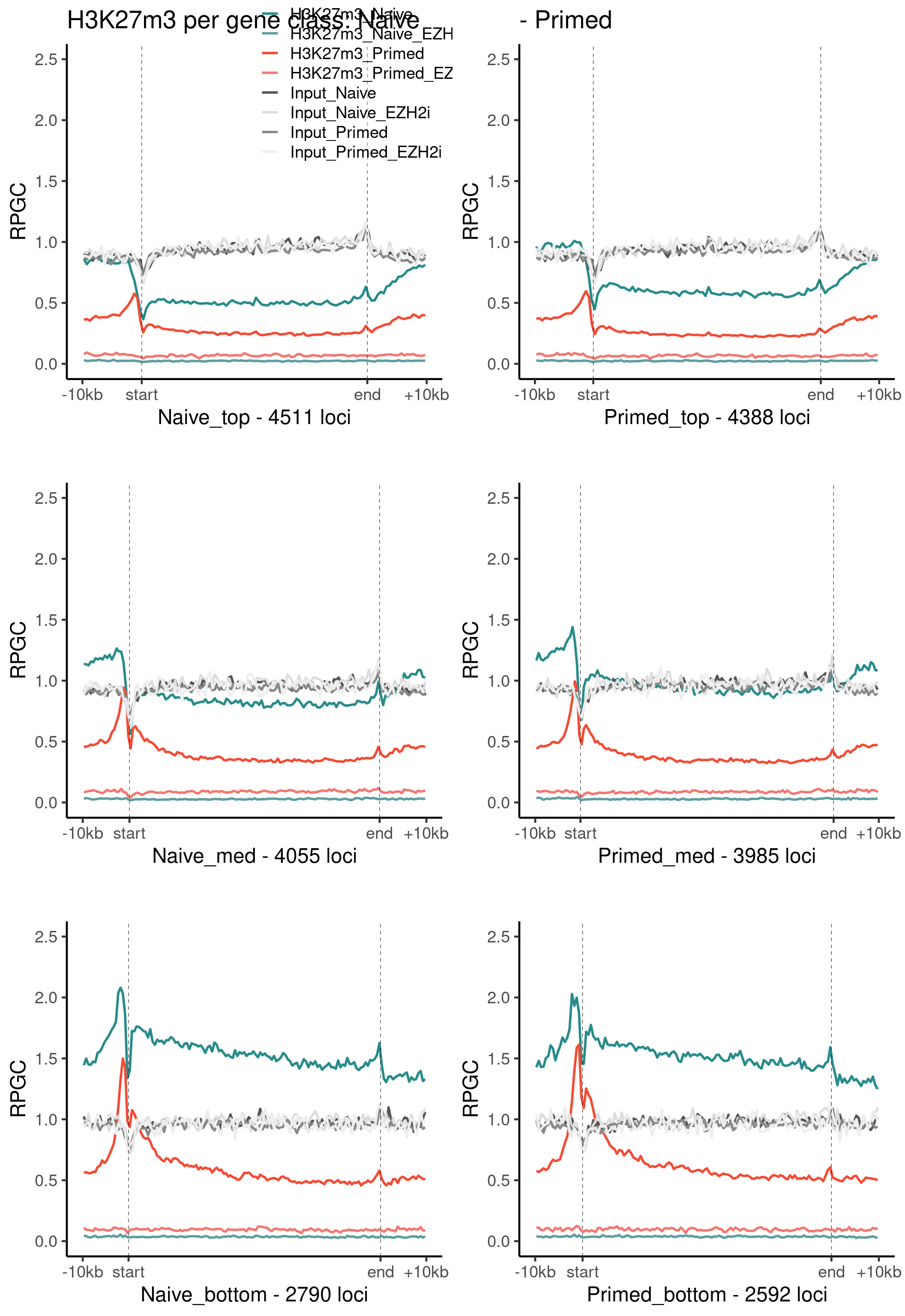
Boxplots
bedfiles_top <- list.files(params$genesdir, full.names = T, pattern = "_top")
bedfiles_med <- list.files(params$genesdir, full.names = T, pattern = "_med")
bedfiles_bottom <- list.files(params$genesdir, full.names = T, pattern = "_bottom")

# Ensures proper order
bedfiles <- c(bedfiles_top, bedfiles_med, bedfiles_bottom)
bwsignal <- bwfiles[grepl("H3K27m3.*pooled.hg38.scaled", bwfiles)]

colors <- as.character(style_info[basename(c(bwsignal, bwinput)), "color_cond"])
labels <- style_info[basename(c(bwsignal, bwinput)), "label"]

# Use tss for this
tss_window <- 2500

bed_ranges <- lapply(bedfiles, import)
tss_ranges <- lapply(bed_ranges, promoters, upstream = tss_window, downstream = tss_window)


this_plot <- partial(bw_loci, bwfiles = c(bwsignal, bwinput))
#
plots <- purrr::map(tss_ranges, this_plot)
names(plots) <- basename(bedfiles)

# Pivot 1 item:
library(tidyr)
Attaching package: 'tidyr'The following object is masked from 'package:S4Vectors':
expandpivot_bed <- function(granges, loci_name) {
bin_ids <- c("seqnames", "start", "end", "width", "strand")
pivoted <- pivot_longer(data = data.frame(granges),
cols = contains("pooled.hg38"),
names_pattern = "(.*)_pooled.hg38.*",
names_to = "sample",
values_to = "value")
pivoted[["group"]] <- loci_name
pivoted
}
pivoted_list <- map2(plots, names(plots), pivot_bed)
all_vals <- do.call(rbind, pivoted_list)
ggplot(all_vals, aes(x = sample, y = value, color = sample, group = sample)) + geom_boxplot() + facet_wrap(group ~ .) + theme_default() + theme(axis.text.x = element_text(angle=45, hjust = 1)) + scale_color_manual(name = "sample", values = colors)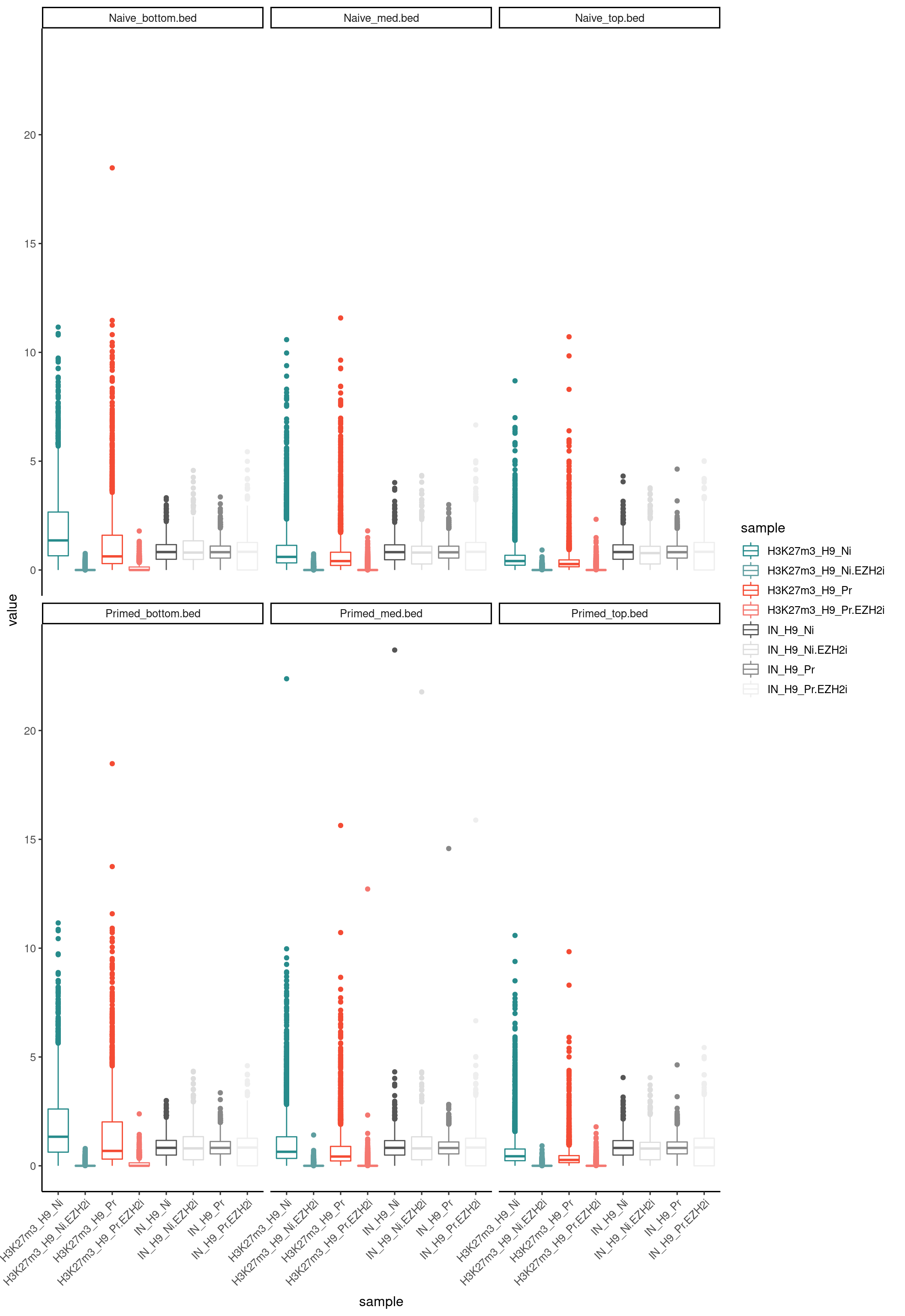
H3K4m3
Highly expressed genes
bedfiles <- list.files(params$genesdir, full.names = T, pattern = "top")
bwfiles <- list.files(params$bwdir, full.names = T)

bwinput <- bwfiles[grepl("IN.*pooled", bwfiles)]
bwsignal <- bwfiles[grepl("H3K4m3.*pooled.hg38.scaled", bwfiles)]

colors <- as.character(style_info[basename(c(bwsignal, bwinput)), "color_cond"])
labels <- style_info[basename(c(bwsignal, bwinput)), "label"]

up <- 10000
dw <- 10000
bs <- 500
md <- "stretch"
global_lims <- c(0, 115)

this_plot <- partial(plot_bw_profile, bwfiles = c(bwsignal, bwinput),
                     bin_size = bs,
                     mode = md,
                     upstream = up,
                     downstream = dw,
                     colors = colors,
                     labels = labels)

plots <- purrr::map(bedfiles, this_plot)
plots[[1]] <- plots[[1]] + ylim(global_lims) + theme(legend.position = "none") + ggtitle("H3K4m3 @Top genes")
plots[[2]] <- plots[[2]] + ylim(global_lims) + ylab("") + ggtitle("")

plot_grid(plotlist=plots, nrow=1)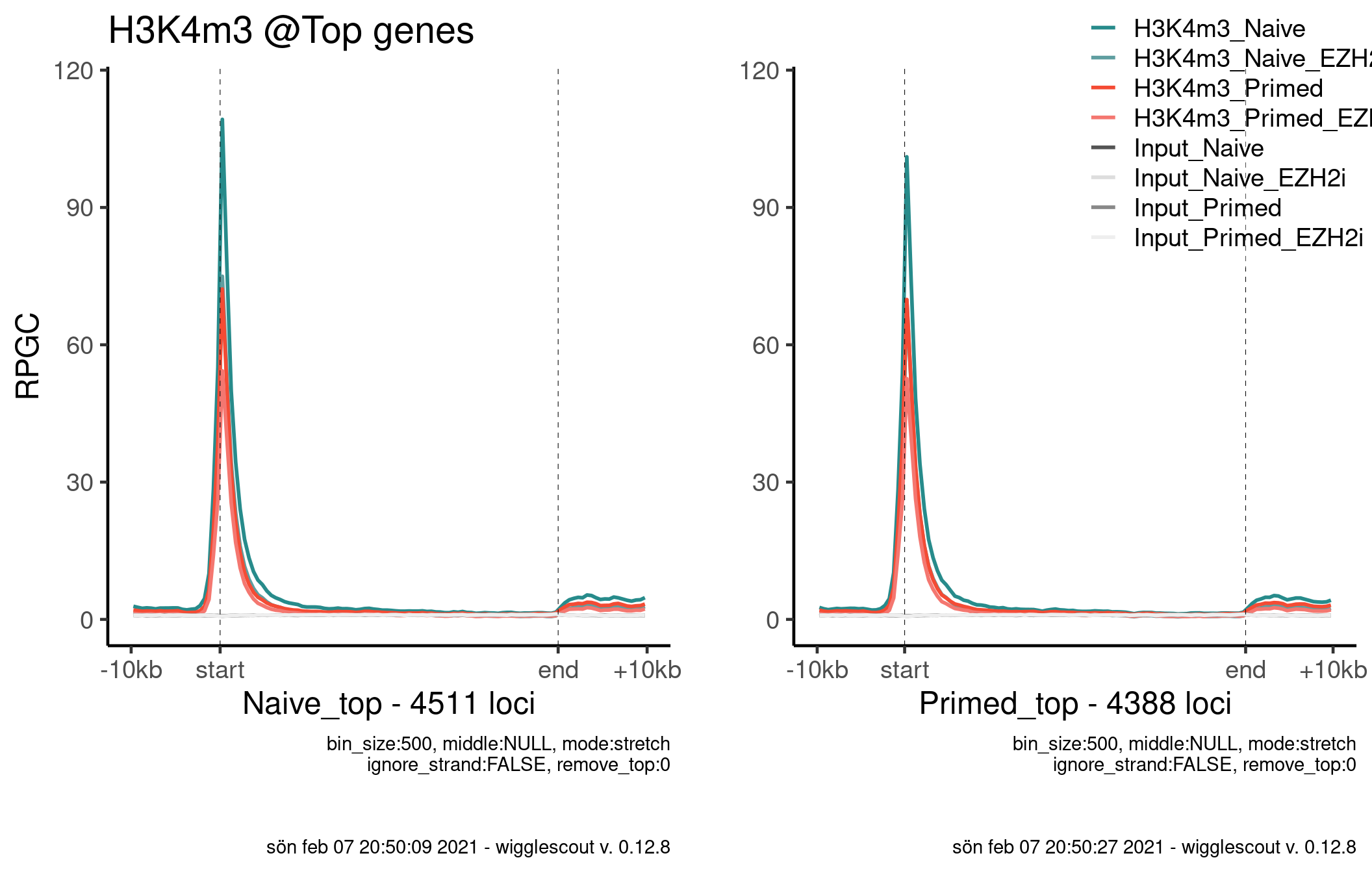
Norm to input
colors <- as.character(style_info[basename(bwsignal), "color_cond"])
labels <- style_info[basename(bwsignal), "label"]

this_plot <- partial(plot_bw_profile, bwfiles = bwsignal, bg_bwfiles = bwinput,
                     bin_size = bs,
                     mode = md,
                     upstream = up,
                     downstream = dw,
                     colors = colors,
                     labels = labels)

plots <- purrr::map(bedfiles, this_plot)
plots[[1]] <- plots[[1]] + ylim(global_lims) + theme(legend.position = "none") + ggtitle("H3K4m3 @Top genes")
plots[[2]] <- plots[[2]] + ylim(global_lims) + ylab("") + ggtitle("")

plot_grid(plotlist=plots, nrow=1)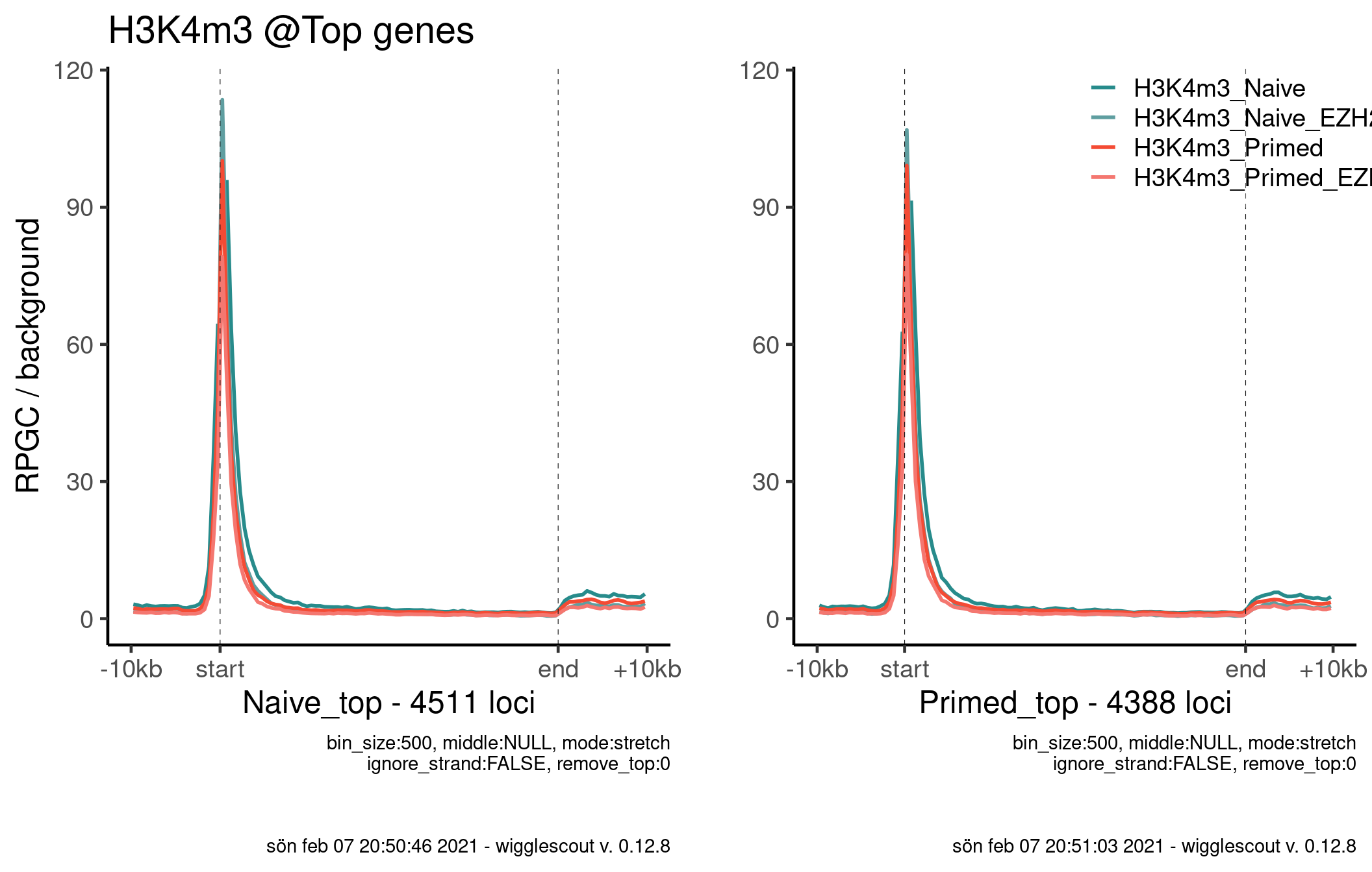
Naive-only vs primed-only
naive_only_top <- setdiff(naive_top, primed_top)
primed_only_top <- setdiff(primed_top, naive_top)
both <- intersect(naive_top, primed_top)

colors <- as.character(style_info[basename(c(bwsignal, bwinput)), "color_cond"])
labels <- style_info[basename(c(bwsignal, bwinput)), "label"]

this_plot <- partial(plot_bw_profile, bwfiles = c(bwsignal, bwinput),
                     bin_size = bs,
                     mode = md,
                     upstream = up,
                     downstream = dw,
                     colors = colors,
                     labels = labels)


plots <- purrr::map(list(naive_only_top, primed_only_top, both), this_plot)
plots[[1]] <- plots[[1]] + ylim(global_lims) + theme(legend.position = "none") + ggtitle("Naive-only")
plots[[2]] <- plots[[2]] + ylim(global_lims) + ylab("") + theme(legend.position = "none") + ggtitle("Primed-only")
plots[[3]] <- plots[[3]] + ylim(global_lims) + ylab("") + ggtitle("Both")

plot_grid(plotlist=plots, ncol=2)
Norm to input:
colors <- as.character(style_info[basename(bwsignal), "color_cond"])
labels <- style_info[basename(bwsignal), "label"]

this_plot <- partial(plot_bw_profile, bwfiles = bwsignal, bg_bwfiles = bwinput,
                     bin_size = bs,
                     mode = md,
                     upstream = up,
                     downstream = dw,
                     colors = colors,
                     labels = labels)


plots <- purrr::map(list(naive_only_top, primed_only_top, both), this_plot)
plots[[1]] <- plots[[1]] + ylim(global_lims) + theme(legend.position = "none") + ggtitle("Naive-only")
plots[[2]] <- plots[[2]] + ylim(global_lims) + ylab("") + theme(legend.position = "none") + ggtitle("Primed-only")
plots[[3]] <- plots[[3]] + ylim(global_lims) + ylab("") + ggtitle("Both")

plot_grid(plotlist=plots, ncol=2)
High-med-low expressed genes
bedfiles_top <- list.files(params$genesdir, full.names = T, pattern = "_top")
bedfiles_med <- list.files(params$genesdir, full.names = T, pattern = "_med")
bedfiles_bottom <- list.files(params$genesdir, full.names = T, pattern = "_bottom")

# Ensures proper order
bedfiles <- c(bedfiles_top, bedfiles_med, bedfiles_bottom)
bwsignal <- bwfiles[grepl("H3K4m3.*pooled.hg38.scaled", bwfiles)]

colors <- as.character(style_info[basename(c(bwsignal, bwinput)), "color_cond"])
labels <- style_info[basename(c(bwsignal, bwinput)), "label"]

up <- 10000
dw <- 10000
bs <- 500
md <- "stretch"
global_lims <- c(0, 115)

this_plot <- partial(plot_bw_profile, bwfiles = c(bwsignal, bwinput),
                     bin_size = bs,
                     mode = md,
                     upstream = up,
                     downstream = dw,
                     colors = colors,
                     labels = labels,
                     verbose = FALSE) # Plot gets too crowded

plots <- purrr::map(bedfiles, this_plot)

plots <- remove_extra_captions(plots)
plots <- set_global_y_axis(plots, global_lims)

plots[[1]] <- plots[[1]] + ggtitle("H3K4m3 per gene class: Naive")
plots[[2]] <- plots[[2]] + ggtitle("Primed" )

plot_grid(plotlist=plots, nrow=3)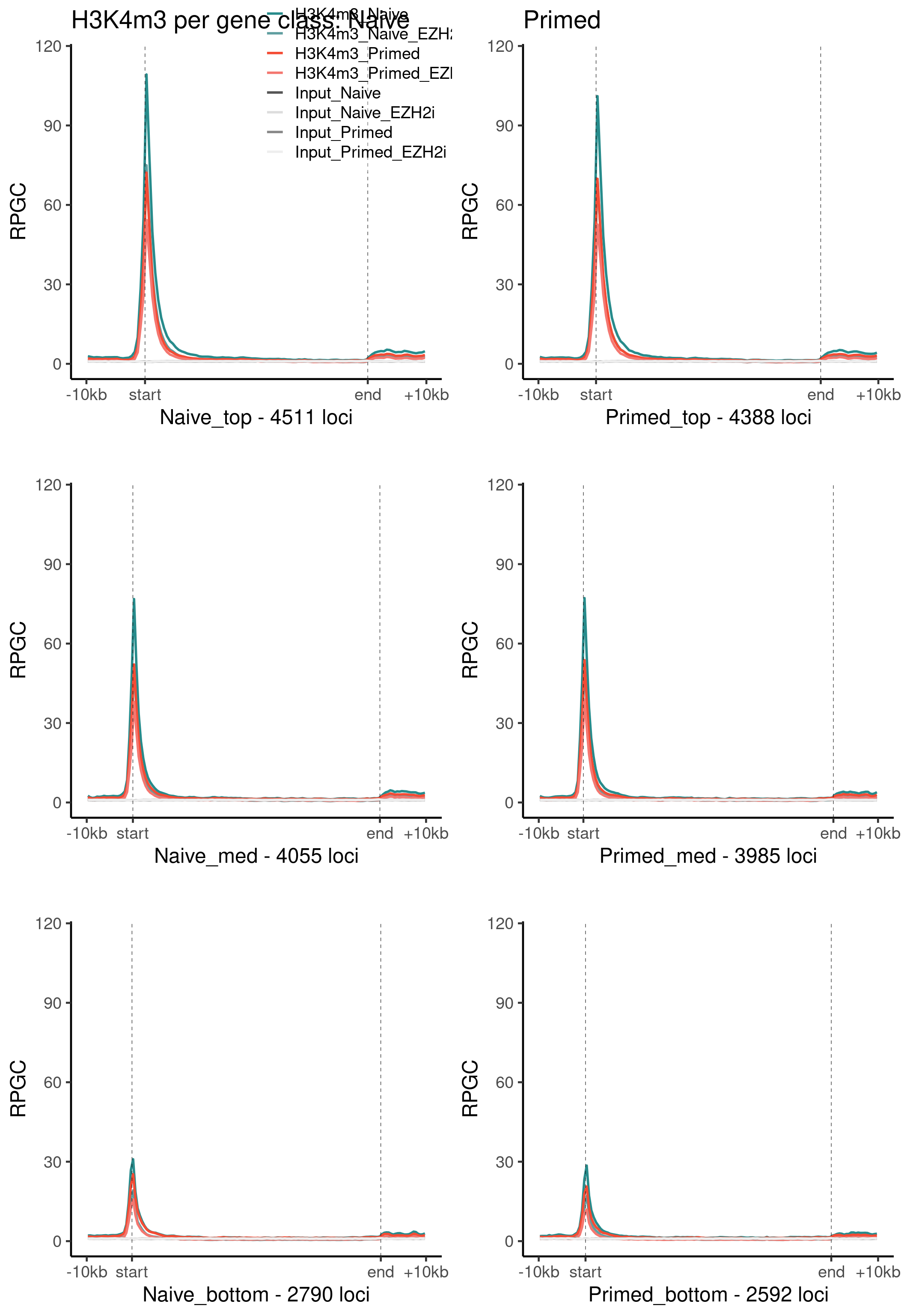
H2AUb
High-med-low expressed genes
bedfiles_top <- list.files(params$genesdir, full.names = T, pattern = "_top")
bedfiles_med <- list.files(params$genesdir, full.names = T, pattern = "_med")
bedfiles_bottom <- list.files(params$genesdir, full.names = T, pattern = "_bottom")

# Ensures proper order
bedfiles <- c(bedfiles_top, bedfiles_med, bedfiles_bottom)
bwsignal <- bwfiles[grepl("H2A.*pooled.hg38.scaled", bwfiles)]

colors <- as.character(style_info[basename(c(bwsignal, bwinput)), "color_cond"])
labels <- style_info[basename(c(bwsignal, bwinput)), "label"]

up <- 10000
dw <- 10000
bs <- 500
md <- "stretch"
global_lims <- c(0, 3)

this_plot <- partial(plot_bw_profile, bwfiles = c(bwsignal, bwinput),
                     bin_size = bs,
                     mode = md,
                     upstream = up,
                     downstream = dw,
                     colors = colors,
                     labels = labels,
                     verbose = FALSE) # Plot gets too crowded

plots <- purrr::map(bedfiles, this_plot)

plots <- remove_extra_captions(plots)
plots <- set_global_y_axis(plots, global_lims)

plots[[1]] <- plots[[1]] + ggtitle("H2AUb per gene class: Naive")
plots[[2]] <- plots[[2]] + ggtitle("Primed" )

plot_grid(plotlist=plots, nrow=3)
sessionInfo()R version 4.0.3 (2020-10-10)
Platform: x86_64-pc-linux-gnu (64-bit)
Running under: Ubuntu 20.04.2 LTS
Matrix products: default
BLAS: /usr/lib/x86_64-linux-gnu/openblas-pthread/libblas.so.3
LAPACK: /usr/lib/x86_64-linux-gnu/openblas-pthread/liblapack.so.3
locale:
[1] LC_CTYPE=en_US.UTF-8 LC_NUMERIC=C
[3] LC_TIME=sv_SE.UTF-8 LC_COLLATE=en_US.UTF-8
[5] LC_MONETARY=sv_SE.UTF-8 LC_MESSAGES=en_US.UTF-8
[7] LC_PAPER=sv_SE.UTF-8 LC_NAME=C
[9] LC_ADDRESS=C LC_TELEPHONE=C
[11] LC_MEASUREMENT=sv_SE.UTF-8 LC_IDENTIFICATION=C
attached base packages:
[1] parallel stats4 grid stats graphics grDevices utils
[8] datasets methods base
other attached packages:
[1] tidyr_1.1.2 cowplot_1.1.1 xfun_0.20
[4] purrr_0.3.4 rtracklayer_1.50.0 GenomicRanges_1.42.0
[7] GenomeInfoDb_1.26.2 IRanges_2.24.1 S4Vectors_0.28.1
[10] BiocGenerics_0.36.0 ggvenn_0.1.8 dplyr_1.0.4
[13] knitr_1.31 ggplot2_3.3.3 wigglescout_0.12.8
[16] workflowr_1.6.2
loaded via a namespace (and not attached):
[1] MatrixGenerics_1.2.0 Biobase_2.50.0
[3] assertthat_0.2.1 highr_0.8
[5] GenomeInfoDbData_1.2.4 Rsamtools_2.6.0
[7] yaml_2.2.1 globals_0.14.0
[9] pillar_1.4.7 lattice_0.20-41
[11] glue_1.4.2 digest_0.6.27
[13] RColorBrewer_1.1-2 promises_1.1.1
[15] XVector_0.30.0 colorspace_2.0-0
[17] htmltools_0.5.1.1 httpuv_1.5.5
[19] Matrix_1.3-2 plyr_1.8.6
[21] XML_3.99-0.5 pkgconfig_2.0.3
[23] listenv_0.8.0 zlibbioc_1.36.0
[25] scales_1.1.1 whisker_0.4
[27] later_1.1.0.1 BiocParallel_1.24.1
[29] git2r_0.28.0 tibble_3.0.6
[31] generics_0.1.0 farver_2.0.3
[33] ellipsis_0.3.1 withr_2.4.1
[35] SummarizedExperiment_1.20.0 furrr_0.2.2
[37] magrittr_2.0.1 crayon_1.4.0
[39] evaluate_0.14 fs_1.5.0
[41] future_1.21.0 parallelly_1.23.0
[43] tools_4.0.3 lifecycle_0.2.0
[45] matrixStats_0.58.0 stringr_1.4.0
[47] munsell_0.5.0 DelayedArray_0.16.0
[49] Biostrings_2.58.0 compiler_4.0.3
[51] rlang_0.4.10 RCurl_1.98-1.2
[53] bitops_1.0-6 labeling_0.4.2
[55] rmarkdown_2.6 gtable_0.3.0
[57] codetools_0.2-18 DBI_1.1.1
[59] reshape2_1.4.4 R6_2.5.0
[61] GenomicAlignments_1.26.0 rprojroot_2.0.2
[63] stringi_1.5.3 Rcpp_1.0.6
[65] vctrs_0.3.6 tidyselect_1.1.0