Last updated: 2021-02-07

Checks: 7 0

Knit directory: hesc-epigenomics/

This reproducible R Markdown analysis was created with workflowr (version 1.6.2). The Checks tab describes the reproducibility checks that were applied when the results were created. The Past versions tab lists the development history.


Great! Since the R Markdown file has been committed to the Git repository, you know the exact version of the code that produced these results.

Great job! The global environment was empty. Objects defined in the global environment can affect the analysis in your R Markdown file in unknown ways. For reproduciblity it’s best to always run the code in an empty environment.

The command set.seed(20210202) was run prior to running the code in the R Markdown file. Setting a seed ensures that any results that rely on randomness, e.g. subsampling or permutations, are reproducible.

Great job! Recording the operating system, R version, and package versions is critical for reproducibility.

Nice! There were no cached chunks for this analysis, so you can be confident that you successfully produced the results during this run.

Great job! Using relative paths to the files within your workflowr project makes it easier to run your code on other machines.

Great! You are using Git for version control. Tracking code development and connecting the code version to the results is critical for reproducibility.

The results in this page were generated with repository version d025037. See the Past versions tab to see a history of the changes made to the R Markdown and HTML files.

Note that you need to be careful to ensure that all relevant files for the analysis have been committed to Git prior to generating the results (you can use wflow_publish or wflow_git_commit). workflowr only checks the R Markdown file, but you know if there are other scripts or data files that it depends on. Below is the status of the Git repository when the results were generated:


Ignored files:
    Ignored:    .Rhistory
    Ignored:    .Rproj.user/
    Ignored:    data/bed/
    Ignored:    data/bw
    Ignored:    data/meta/
    Ignored:    data/peaks
    Ignored:    data/rnaseq/

Untracked files:
    Untracked:  analysis/gene_expression_groups.Rmd
    Untracked:  output/Collier_2017/ensembl/

Unstaged changes:
    Modified:   analysis/index.Rmd
    Modified:   output/Collier_2017/Naive_bottom.bed
    Modified:   output/Collier_2017/Naive_med.bed
    Modified:   output/Collier_2017/Primed_bottom.bed
    Modified:   output/Collier_2017/Primed_med.bed

Note that any generated files, e.g. HTML, png, CSS, etc., are not included in this status report because it is ok for generated content to have uncommitted changes.


These are the previous versions of the repository in which changes were made to the R Markdown (analysis/rna_seq_collier_2017.Rmd) and HTML (docs/rna_seq_collier_2017.html) files. If you’ve configured a remote Git repository (see ?wflow_git_remote), click on the hyperlinks in the table below to view the files as they were in that past version.

File Version Author Date Message
Rmd d025037 cnluzon 2021-02-07 wflow_publish(“analysis/rna_seq_collier_2017.Rmd”)
Rmd 0481b52 cnluzon 2021-02-05 RNA seq first analysis
html 0481b52 cnluzon 2021-02-05 RNA seq first analysis

Summary

Data: Used public data from (Collier et al. 2017): H9 embryonic stem cells in Naïve and Primed state, three biological replicates.

Sample info
dataset_id gsm_id description filename run_id input layout experiment
26 Collier_2017 GSM2449055 hESC_H9_naive_1 hESC_H9_naive_1 SRR5151102 - single RNA-seq
27 Collier_2017 GSM2449056 hESC_H9_naive_2 hESC_H9_naive_2 SRR5151103 - single RNA-seq
28 Collier_2017 GSM2449057 hESC_H9_naive_3 hESC_H9_naive_3 SRR5151104 - single RNA-seq
29 Collier_2017 GSM2449058 hESC_H9_primed_1 hESC_H9_primed_1 SRR5151105 - single RNA-seq
30 Collier_2017 GSM2449059 hESC_H9_primed_2 hESC_H9_primed_2 SRR5151106 - single RNA-seq
31 Collier_2017 GSM2449060 hESC_H9_primed_3 hESC_H9_primed_3 SRR5151107 - single RNA-seq

Primary analysis

RNA-seq data was analysed by a standard RNA-seq pipeline v2.0, available on nf-core (Ewels et al. 2019) with mostly default settings. For more information about the specific steps involved in this analysis, refer to the repository documentation: https://nf-co.re/rnaseq/2.0.

Reference genome

Due to some difficulties in using hg38 with iGenomes, and since the rest of the analysis has been done on such reference (more specifically, GRCh38.p12). An annotation was downloaded from Ensembl and used as matching custom --fasta and --gtf parameters:

ftp://ftp.ensembl.org/pub/release-95/gtf/homo_sapiens/Homo_sapiens.GRCh38.95.gtf.gz

ftp://ftp.ensembl.org/pub/release-95/fasta/homo_sapiens/dna/Homo_sapiens.GRCh38.dna_sm.primary_assembly.fa.gz

Running environment

RNA-seq analysis was run on Uppmax HPC environment using standard parameters: nextflow run nf-core/rnaseq -profile uppmax -revision 2.0 --public_data_ids ids_file.txt. ids_file.txt contained only the GSM ids as plain text.

This run would produce the corresponding FASTQ files and then a further run with the generated samplesheet_grouped.tsv file, the pipeline was run.

Note on pipeline version

There is a newer RNA-seq version: https://github.com/nf-core/rnaseq/releases/tag/3.0. This affects the quantification, so it may be the case that results are better using Salmon instead of featureCounts. However at this point there is a problem with Singularity on Uppmax and this version cannot be easily run. If necessary, I will re-do this analysis in the future, once these problems are solved.

Downstream analysis

Helper functions

color_list <- c(Naive=global_palette$teal,
                Primed=global_palette$coral)

#' Subset a stringtie output table intro high/med/low expr genes
#'
#' @param counts Counts table.
#' @param min_length Gene length cutoff.
#' @param group_size Number of genes per group.
#' @param min_cutoff Minimum threshold to consider.
#' @param field Which field to use (default = TPM).
#'
#' @return Named list top, bottom, med
categorize_genes <- function(counts, min_length, group_size, min_cutoff = 0, field = "TPM") {
  counts$length <- (counts$End - counts$Start)

  # Filter by gene length
  counts <- counts[counts$length > min_length, ]
  
  # Count as "low" genes that have something, instead of none?
  counts <- counts[counts[, field] > min_cutoff, ]
  
  # Sort by corresponding column
  counts <- counts[order(counts[, field], decreasing = TRUE), ]
  
  total <- nrow(counts)
  
  top <- counts[1:group_size, ]
  bottom <- counts[(total-group_size+1):total, ]
  med <- counts[((total/2)-(group_size/2)):((total/2)+(group_size/2)-1),]
  
  list(top = top, bottom = bottom, med = med)
}

#' Make a venn diagram out ouf a list of selected gene counts
#'
#' @param lists List of lists of three (top, med, bottom) gene counts.
#' @param field Which group to select (top, med, bottom)-
#' @param title Plot title
#' @param color Base color

#' @return ggplot object
genes_venn <- function(lists, field, title, color) {
  field_list <- list(r1 = lists[[1]][[field]]$Gene.Name, 
                     r2 = lists[[2]][[field]]$Gene.Name,
                     r3 = lists[[3]][[field]]$Gene.Name)
  
  clist <- rep(color, 3)
  ggvenn(field_list, fill_color = clist, fill_alpha = 0.5, text_size = 5, stroke_color = "#ffffff") + 
    ggtitle(title)
}

#' Intersect per category
#'
#' @param group_list List of lists of three (top, med, bottom) gene counts.
#' @param category Which group to select (top, med, bottom).
#'
#' @return Gene names that intersect
intersect_3 <- function(group_list, category) {
  intersect(intersect(group_list[[1]][[category]]$Gene.Name,
                      group_list[[2]][[category]]$Gene.Name),
            group_list[[3]][[category]]$Gene.Name)
}

#' Subset a named granges by name
#'
#' @param names Names list
#' @param granges GRanges to subset.
#'
#' @return GRanges
select_genes <- function(names, granges) {
  sort(granges[granges$name %in% names, ])
}

#' Get GRanges with gene symbols for hg38
#'
#' @return A GRanges where name field is Gene symbol
genes_hg38 <- function() {
  # This matches gene IDs to symbols
  x <- org.Hs.egSYMBOL
  
  # Get the gene names that are mapped to an entrez gene identifier
  mapped_genes <- mappedkeys(x)
  # Convert to a list
  xx <- as.list(x[mapped_genes])
  
  # Apparently there are some pathway crap that puts NAs in the list
  xx <- xx[!is.na(xx)]
  
  gene_id_to_name <- unlist(xx)
  
  genes <- genes(TxDb.Hsapiens.UCSC.hg38.knownGene)
  genes$name <- gene_id_to_name[genes$gene_id]
  genes
}

#' Get GRanges with gene symbols for hg38
#'
#' @return A GRanges where name field is Gene symbol
genes_hg38_ensembl <- function() {
  # This matches gene IDs to symbols
  edb <- EnsDb.Hsapiens.v86
  genes(edb)
}


#' Export gene sets out of a list of selected gene counts
#'
#' @param group_list List of lists of three (top, med, bottom) gene counts.
#' @param prefix File name prefix
export_gene_sets_ensembl <- function(group_list, prefix) {
  merged <- map(c("top", "med", "bottom"),
                   intersect_3,
                   group_list=group_list)
  
  out_files <- paste0(file.path("./output/Collier_2017/ensembl/",
                      paste(prefix,
                            c("top.bed", "med.bed", "bottom.bed"), sep="_")))
  
  genes_all <- genes_hg38_ensembl()
  genes_all <- genes_all[, "gene_name"] 
  names(mcols(genes_all)) <- "name"
  
  ranges_list <- map(merged, select_genes, granges=genes_all)
  
  file_list <- map2(ranges_list, out_files, export)
}


#' Export gene sets out of a list of selected gene counts
#'
#' @param group_list List of lists of three (top, med, bottom) gene counts.
#' @param prefix File name prefix
export_gene_sets <- function(group_list, prefix) {
  merged <- map(c("top", "med", "bottom"),
                   intersect_3,
                   group_list=group_list)
  
  out_files <- paste0(file.path("./output/Collier_2017/"),
                      paste(prefix,
                            c("top.bed", "med.bed", "bottom.bed"), sep="_"))
  
  genes_all <- genes_hg38()

  ranges_list <- map(merged, select_genes, granges=genes_all)
  
  file_list <- map2(ranges_list, out_files, export)
}

Gene counts

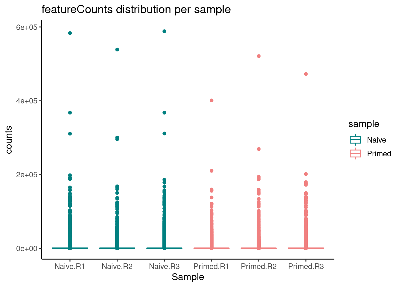
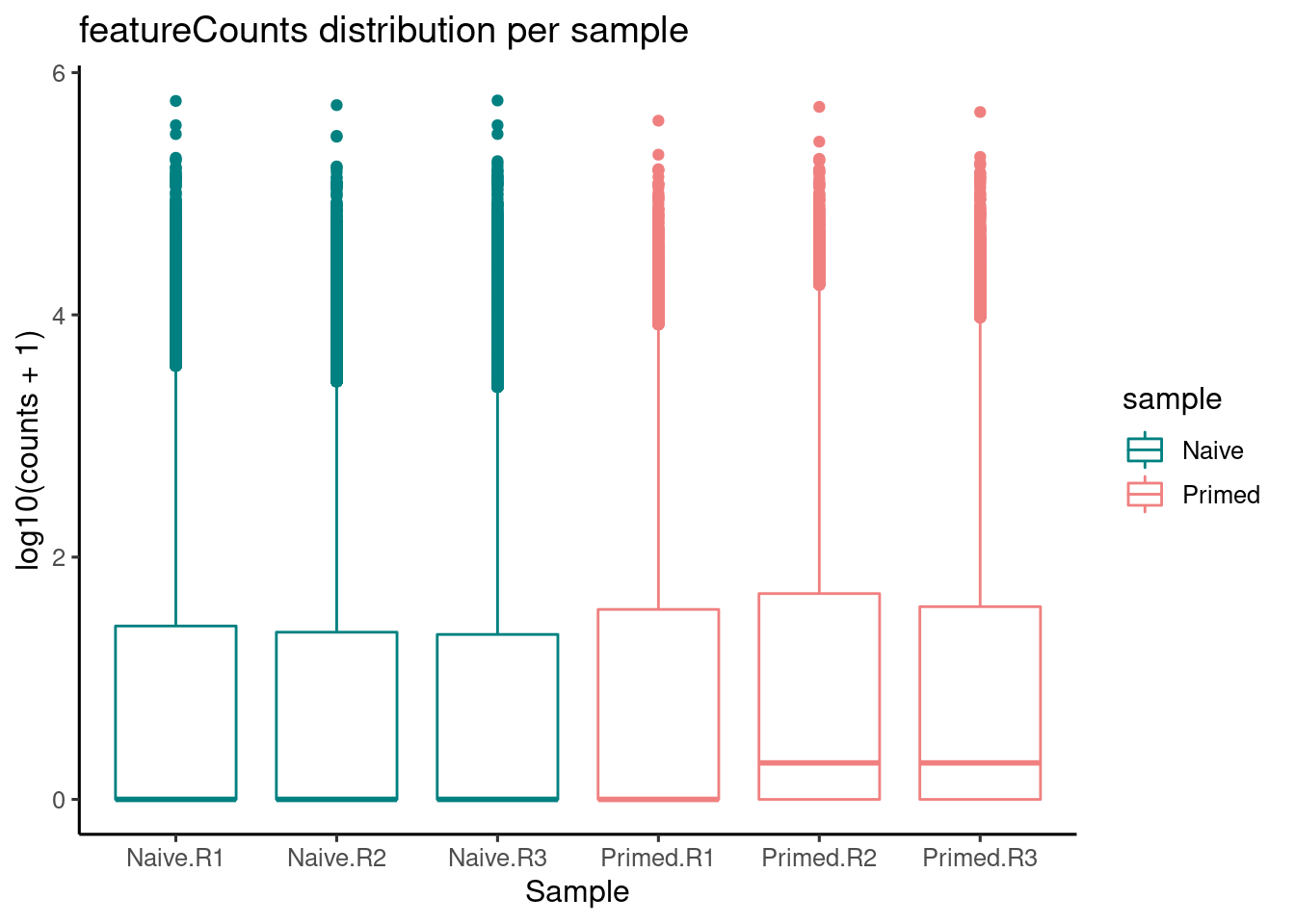
Gene counts output file from featureCounts are used.

counts_file <- file.path(params$rnaseqdir,
                         "Collier_2017_featurecounts.tsv")

counts <- read.table(counts_file, sep = "\t", header = T)
kable(head(counts))
Geneid gene_name Naive_R1 Naive_R2 Naive_R3 Primed_R1 Primed_R2 Primed_R3
ENSG00000223972 DDX11L1 1 0 0 0 0 2
ENSG00000227232 WASH7P 14 14 10 18 20 24
ENSG00000278267 MIR6859-1 4 3 2 7 6 9
ENSG00000243485 MIR1302-2HG 3 0 0 4 0 4
ENSG00000284332 MIR1302-2 0 0 0 0 0 0
ENSG00000237613 FAM138A 0 0 0 0 0 0

Counts distribution

counts_long <- pivot_longer(counts,
                            cols = -c(Geneid, gene_name),
                            names_to = c("sample", "replicate"),
                            names_sep = "_",
                            values_to = "count",
                            names_ptypes = list(sample = factor(),
                                                replicate = factor()))

color_scale <- scale_color_manual(name = "sample",
                                  values = unlist(color_list))


ggplot(counts_long,
       aes(x = interaction(sample, replicate, lex.order =T),
           y = count, color = sample)) + 
  labs(x = "Sample", y = "counts",
     title = "featureCounts distribution per sample") +
  geom_boxplot() +  
  color_scale + 
  theme_default()

Version Author Date
0481b52 cnluzon 2021-02-05

Log scaled + 1:

library(tidyr)
counts_long <- pivot_longer(counts,
                            cols = -c(Geneid, gene_name),
                            names_to = c("sample", "replicate"),
                            names_sep = "_",
                            values_to = "count",
                            names_ptypes = list(sample = factor(),
                                                replicate = factor()))

color_scale <- scale_color_manual(name = "sample",
                                  values = unlist(color_list))


ggplot(counts_long,
       aes(x = interaction(sample, replicate, lex.order =T),
           y = log10(count+1), color = sample)) + 
  geom_boxplot() +  
  color_scale + 
  labs(x = "Sample", y = "log10(counts + 1)",
       title = "featureCounts distribution per sample") +
  theme_default()

Version Author Date
0481b52 cnluzon 2021-02-05

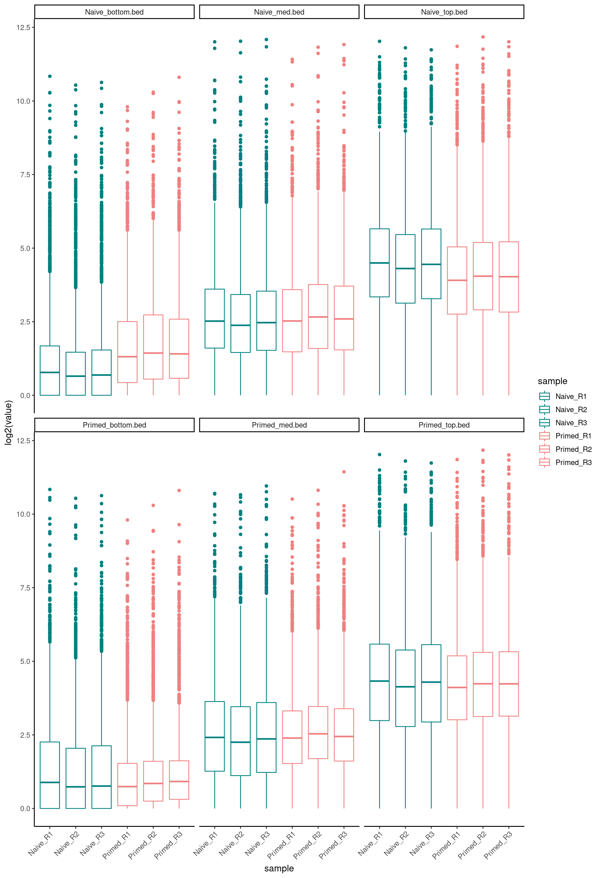
As expected, there are many zero values in all the distributions, and long tails since there is no upper limit in RNA-seq data.

Stringtie output

stringtie (Kovaka et al. 2019) https://ccb.jhu.edu/software/stringtie/) is a tool for quantitation of full-length transcripts (taking variants into account) per gene.

This output is also provided as standard output for RNA-seq pipeline v2.0.

stringtie_files <- list(
  naive = list.files(params$rnaseqdir,
                     pattern = "Naive.*gene_abundance.txt", full.names = T),
  primed = list.files(params$rnaseqdir,
                      pattern = "Primed.*gene_abundance.txt", full.names = T)
)

kable(head(read.csv(stringtie_files$primed[1], header = T, sep = "\t")))
Gene.ID Gene.Name Reference Strand Start End Coverage FPKM TPM
ENSG00000223972 DDX11L1 1 + 11869 14409 0.368065 0.080012 0.162290
ENSG00000227232 WASH7P 1 - 14404 29570 36.709293 6.948467 14.093770
ENSG00000278267 MIR6859-1 1 - 17369 17436 21.787683 4.124051 8.364929
ENSG00000243485 MIR1302-2HG 1 + 29554 31109 1.308571 0.379904 0.770571
ENSG00000284332 MIR1302-2 1 + 30366 30503 0.062616 0.011852 0.024040
ENSG00000237613 FAM138A 1 - 34554 36081 0.173298 0.067773 0.137466

Gene expression groups

To get sets of high - med -low expressed:

1. Remove genes that are shorter than 10kb.

2. Take top 5000, around-median 5000 and lowest 5000 genes.

In this case, we have 3 biological replicates per condition.

So one possible approach is do this per replicate and see how they intersect.

counts_naive <- lapply(stringtie_files$naive,
                       read.csv,
                       header = T,
                       sep = "\t")

min_length_cutoff <- 10000
group_size <- 5000
min_expr_cutoff <- 0
deciding_stat <- "FPKM"

# Set a cutoff for the low expressed genes, so there is still some signal
# In there. When intersecting otherwise, I get few overlap.
groups_naive <- lapply(counts_naive,
                       categorize_genes,
                       min_length = min_length_cutoff,
                       group_size = group_size,
                       min_cutoff = min_expr_cutoff,
                       field = deciding_stat)


counts_primed <- lapply(stringtie_files$primed,
                        read.csv,
                        header = T,
                        sep = "\t")

groups_primed <- lapply(counts_primed,
                        categorize_genes,
                        min_length = min_length_cutoff,
                        group_size = group_size,
                        min_cutoff = min_expr_cutoff,
                        field = deciding_stat)


c <- color_list[["Naive"]]

Naïve expressed gene groups

Top expressed genes:

groups <- groups_naive

genes_venn(groups,
           "top",
           "Naïve top 5k expressed genes across replicates",
           color = c)

Version Author Date
0481b52 cnluzon 2021-02-05

Medium expressed genes:

genes_venn(groups,
           "med",
           "Naïve med 5k expressed genes across replicates",
           color = c)

Version Author Date
0481b52 cnluzon 2021-02-05

Low expressed genes:

genes_venn(groups,
           "bottom",
           "Naïve bottom 5k expressed genes across replicates",
           color = c)

Version Author Date
0481b52 cnluzon 2021-02-05

Primed expressed gene groups

c <- color_list[["Primed"]]

groups <- groups_primed

genes_venn(groups,
           "top",
           "Primed top 5k expressed genes across replicates",
           color = c)

Version Author Date
0481b52 cnluzon 2021-02-05
genes_venn(groups,
           "med",
           "Primed med 5k expressed genes across replicates",
           color = c)

Version Author Date
0481b52 cnluzon 2021-02-05
genes_venn(groups,
           "bottom",
           "Primed low 5k expressed genes across replicates",
           color = c)

Version Author Date
0481b52 cnluzon 2021-02-05

I assume here there should be some overlap

naive_top_genes <- intersect(intersect(groups_naive[[1]]$top$Gene.Name, 
                             groups_naive[[2]]$top$Gene.Name),
                             groups_naive[[3]]$top$Gene.Name)

primed_top_genes <- intersect(intersect(groups_primed[[1]]$top$Gene.Name, 
                              groups_primed[[2]]$top$Gene.Name),
                              groups_primed[[3]]$top$Gene.Name)

field_list <- list(naive=naive_top_genes,
                   primed=primed_top_genes)

ggvenn(field_list, fill_color = c(color_list[["Naive"]], color_list[["Primed"]]), fill_alpha = 0.5, text_size = 5, stroke_color = "#ffffff") + 
    ggtitle("Naive vs primed top expressed genes")

Version Author Date
0481b52 cnluzon 2021-02-05

Gene set enrichment

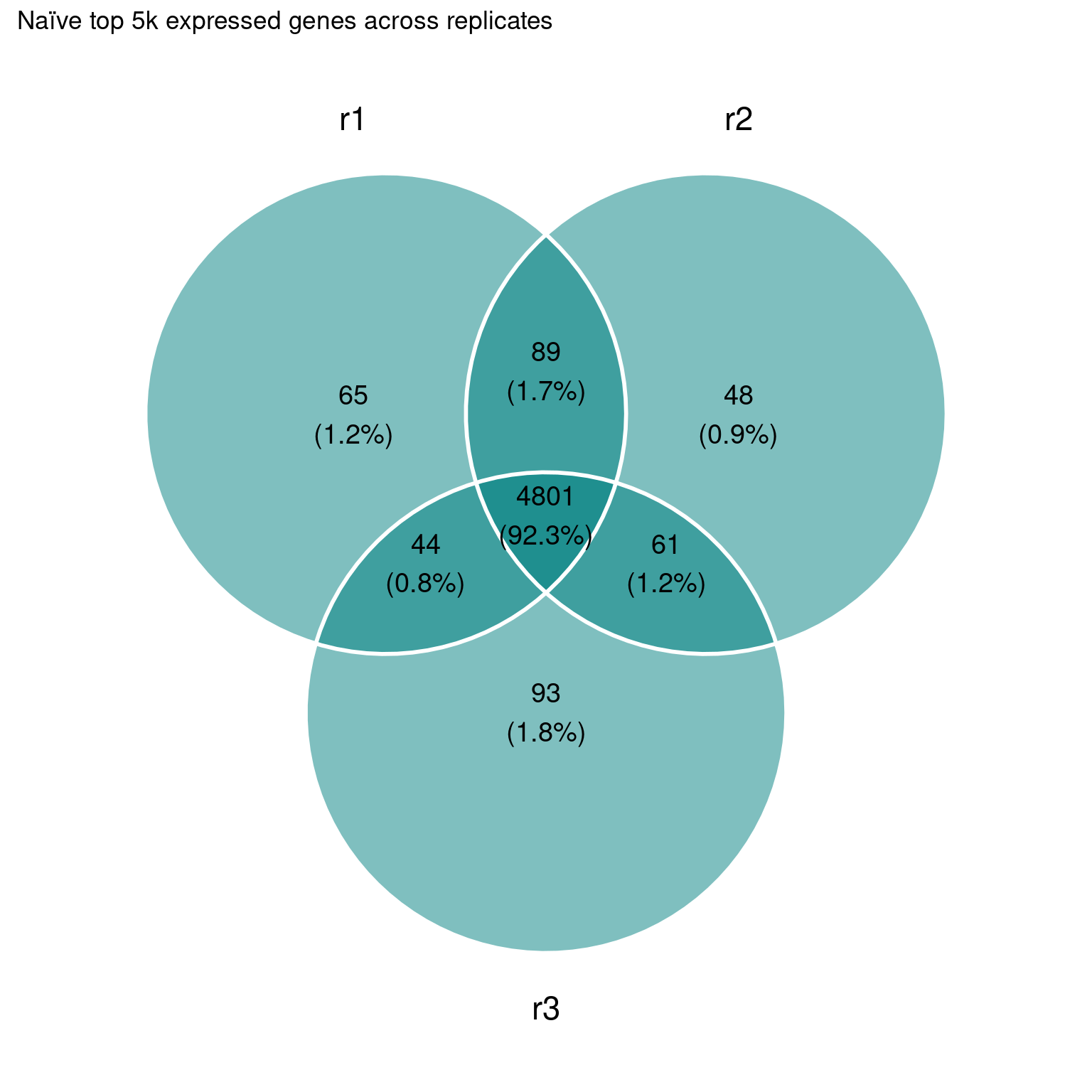
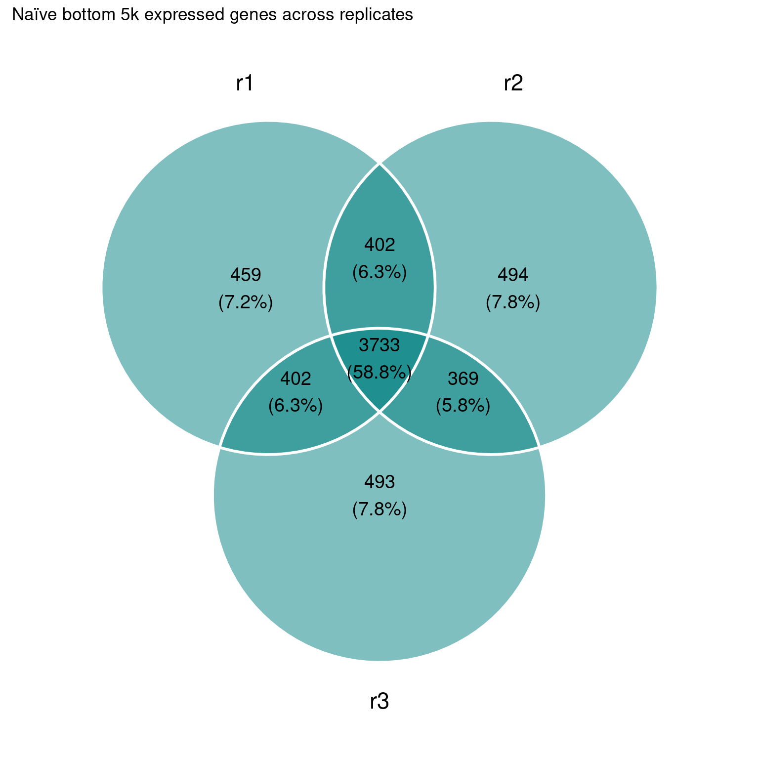
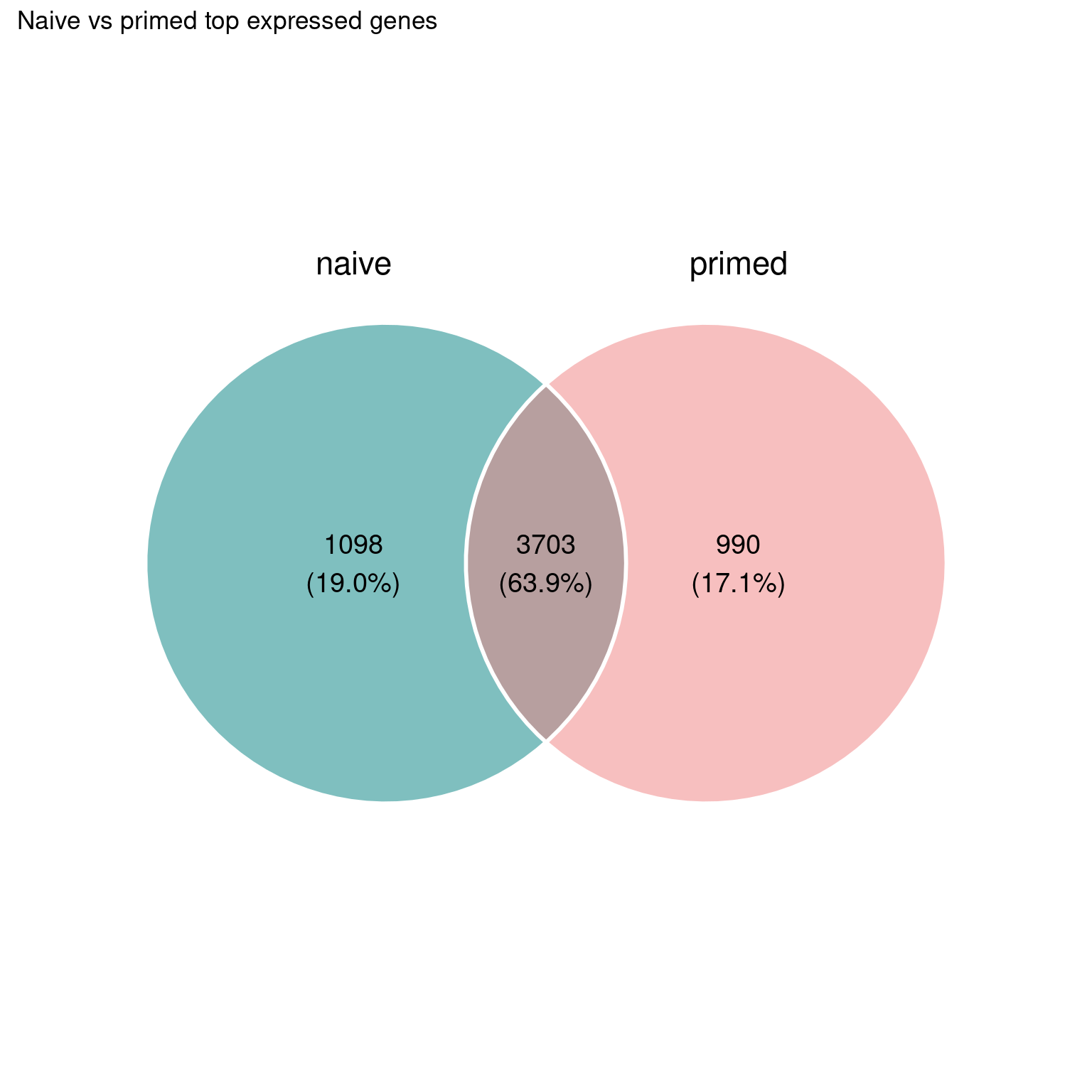
There seems to be some overlap in the Naïve-only vs Primed-only and our groups, when looking at functional annotation, at least. Being more stringent in the top expressed genes:

min_length_cutoff <- 10000
group_size <- 2000
min_expr_cutoff <- 0
deciding_stat <- "TPM"

# Set a cutoff for the low expressed genes, so there is still some signal
# In there. When intersecting otherwise, I get few overlap.
groups_naive <- lapply(counts_naive,
                       categorize_genes,
                       min_length = min_length_cutoff,
                       group_size = group_size,
                       min_cutoff = min_expr_cutoff,
                       field = deciding_stat)


counts_primed <- lapply(stringtie_files$primed,
                        read.csv,
                        header = T,
                        sep = "\t")

groups_primed <- lapply(counts_primed,
                        categorize_genes,
                        min_length = min_length_cutoff,
                        group_size = group_size,
                        min_cutoff = min_expr_cutoff,
                        field = deciding_stat)

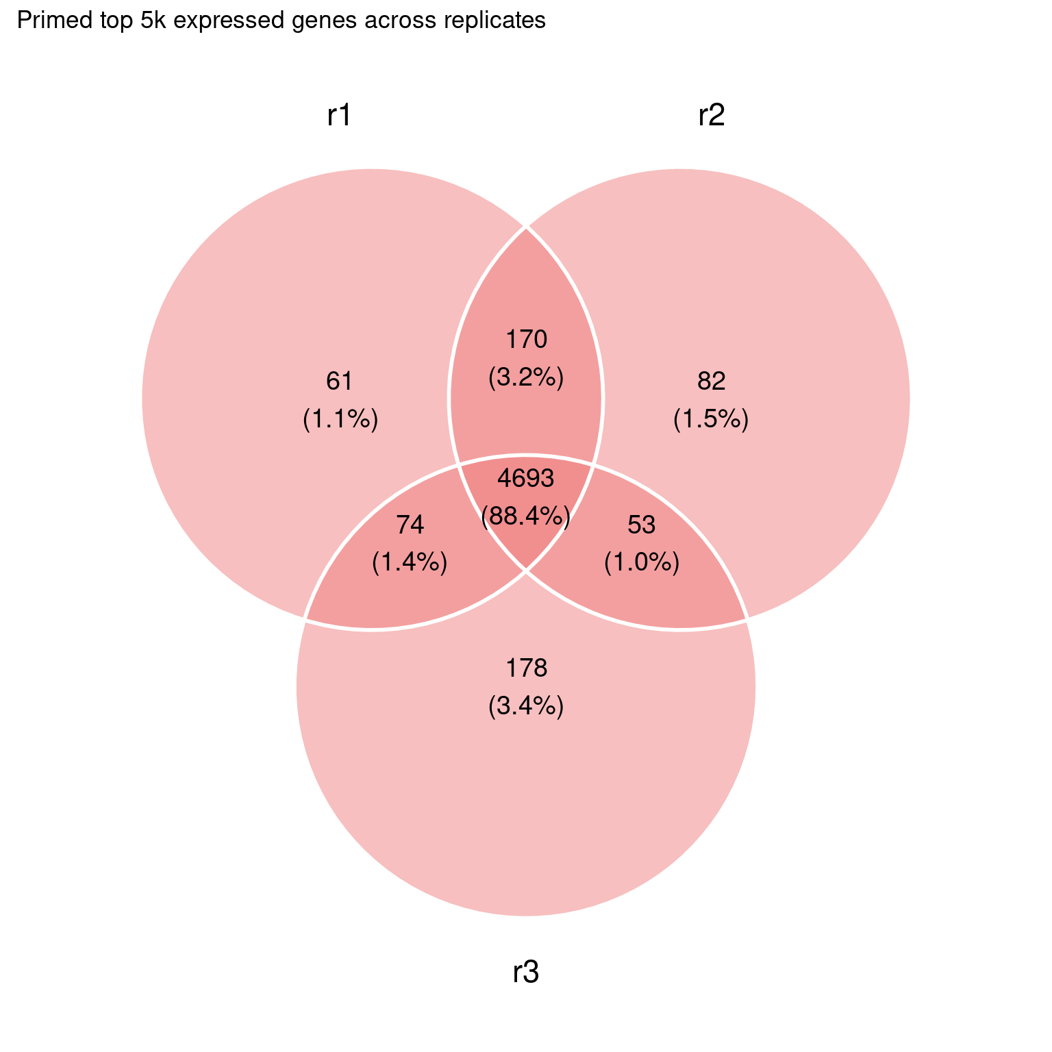
Still quite some overlap among the highest expressed genes:

naive_top_genes <- intersect(intersect(groups_naive[[1]]$top$Gene.Name, 
                             groups_naive[[2]]$top$Gene.Name),
                             groups_naive[[3]]$top$Gene.Name)

primed_top_genes <- intersect(intersect(groups_primed[[1]]$top$Gene.Name, 
                              groups_primed[[2]]$top$Gene.Name),
                              groups_primed[[3]]$top$Gene.Name)

field_list <- list(naive=naive_top_genes,
                   primed=primed_top_genes)

ggvenn(field_list, fill_color = c(color_list[["Naive"]], color_list[["Primed"]]), fill_alpha = 0.5, text_size = 5, stroke_color = "#ffffff") + 
    ggtitle("Naive vs primed top expressed genes")

Version Author Date
0481b52 cnluzon 2021-02-05

Gene enrichment analysis

naive_only <- setdiff(naive_top_genes, primed_top_genes)
primed_only <- setdiff(primed_top_genes, naive_top_genes)
both <- intersect(naive_top_genes, primed_top_genes)

genes <- list(naive_only = naive_only,
              primed_only = primed_only,
              shared = both)

# Do a gprofiler analysis
gostres <- gost(query = genes, 
                organism = "hsapiens", ordered_query = FALSE, 
                multi_query = FALSE, significant = TRUE, exclude_iea = FALSE, 
                measure_underrepresentation = FALSE, evcodes = FALSE, 
                user_threshold = 0.05, correction_method = "g_SCS", 
                domain_scope = "annotated", custom_bg = NULL, 
                numeric_ns = "", sources = NULL, as_short_link = FALSE)

gostplot(gostres, capped = TRUE, interactive = TRUE)

This is a bit too much at the moment, we can probably refine this.

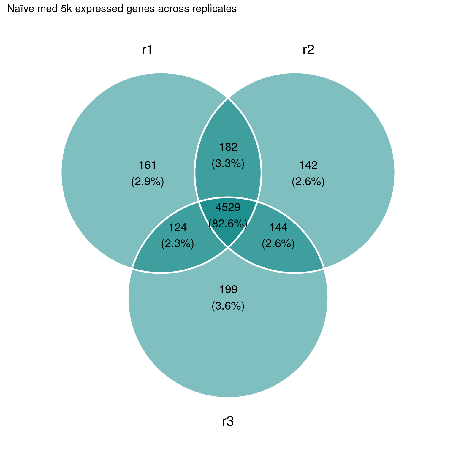
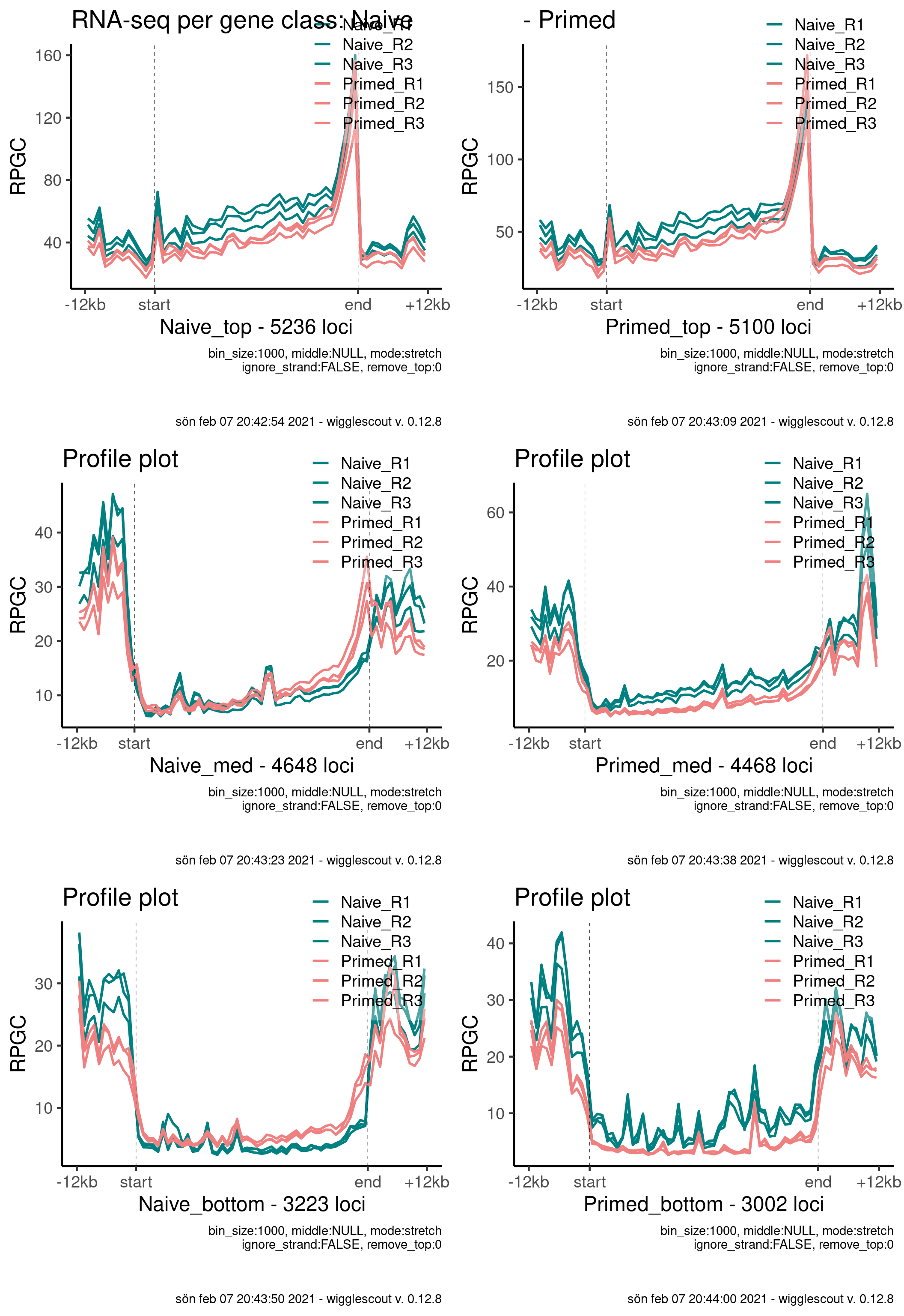
Annotation of gene groups

Now I annotate the intersection of these sets in the reference genome, to be able to look at chromatin marks there.

min_length_cutoff <- 10000
group_size <- 5000
min_expr_cutoff <- 0
deciding_stat <- "TPM"

# Set a cutoff for the low expressed genes, so there is still some signal
# In there. When intersecting otherwise, I get few overlap.
groups_naive <- lapply(counts_naive,
                       categorize_genes,
                       min_length = min_length_cutoff,
                       group_size = group_size,
                       min_cutoff = min_expr_cutoff,
                       field = deciding_stat)

export_gene_sets(groups_naive, "Naive")
  1613 genes were dropped because they have exons located on both strands
  of the same reference sequence or on more than one reference sequence,
  so cannot be represented by a single genomic range.
  Use 'single.strand.genes.only=FALSE' to get all the genes in a
  GRangesList object, or use suppressMessages() to suppress this message.
export_gene_sets_ensembl(groups_naive, "Naive")

groups_naive <- lapply(counts_primed,
                       categorize_genes,
                       min_length = min_length_cutoff,
                       group_size = group_size,
                       min_cutoff = min_expr_cutoff,
                       field = deciding_stat)

export_gene_sets(groups_naive, "Primed")
  1613 genes were dropped because they have exons located on both strands
  of the same reference sequence or on more than one reference sequence,
  so cannot be represented by a single genomic range.
  Use 'single.strand.genes.only=FALSE' to get all the genes in a
  GRangesList object, or use suppressMessages() to suppress this message.
export_gene_sets_ensembl(groups_naive, "Primed")

Download the BED files

Download Collier_2017.zip

RNA-seq bigwig signal at selected groups

This is sort of a validation of the groups I get:

export_dir <- "./output/Collier_2017/ensembl/"
bedfiles_top <- list.files(export_dir, full.names = T, pattern = "_top")
bedfiles_med <- list.files(export_dir, full.names = T, pattern = "_med")
bedfiles_bottom <- list.files(export_dir, full.names = T, pattern = "_bottom")

# Ensures proper order
bedfiles <- c(bedfiles_top, bedfiles_med, bedfiles_bottom)
bwsignal <- list.files(file.path(params$datadir, "bw/Collier_2017"), full.names = T)

colors <- c(rep(color_list[["Naive"]], 3), rep(color_list[["Primed"]], 3))
# labels <- style_info[basename(c(bwsignal, bwinput)), "label"]

# Use tss for this
tss_window <- 2500

bed_ranges <- lapply(bedfiles, import)
tss_ranges <- lapply(bed_ranges, promoters, upstream = tss_window, downstream = tss_window)

this_plot <- partial(bw_loci, bwfiles = bwsignal)
# 
plots <- purrr::map(tss_ranges, this_plot)
names(plots) <- basename(bedfiles)

# Pivot 1 item:
library(tidyr)

pivot_bed <- function(granges, loci_name) {
  bin_ids <- c("seqnames", "start", "end", "width", "strand")
  pivoted <- pivot_longer(data = data.frame(granges),
                             cols = contains("_R"),
                             names_to = "sample",
                             values_to = "value")
  pivoted[["group"]] <- loci_name
  pivoted
}

pivoted_list <- map2(plots, names(plots), pivot_bed)
all_vals <- do.call(rbind, pivoted_list)

ggplot(all_vals, aes(x = sample, y = log2(value), color = sample, group = sample)) + geom_boxplot() + facet_wrap(group ~ .)  + theme_default() + theme(axis.text.x = element_text(angle=45, hjust = 1)) + scale_color_manual(name = "sample", values = colors)

Profile is not very informative, I think.

export_dir <- "./output/Collier_2017/ensembl/"
bedfiles_top <- list.files(export_dir, full.names = T, pattern = "_top")
bedfiles_med <- list.files(export_dir, full.names = T, pattern = "_med")
bedfiles_bottom <- list.files(export_dir, full.names = T, pattern = "_bottom")

# Ensures proper order
bedfiles <- c(bedfiles_top, bedfiles_med, bedfiles_bottom)
bwsignal <- list.files(file.path(params$datadir, "bw/Collier_2017"), full.names = T)

# colors <- as.character(style_info[basename(c(bwsignal, bwinput)), "color_cond"])
# labels <- style_info[basename(c(bwsignal, bwinput)), "label"]

colors <- c(rep(color_list[["Naive"]], 3), rep(color_list[["Primed"]], 3))

up <- 12000
dw <- 12000
bs <- 1000
md <- "stretch"

this_plot <- partial(plot_bw_profile, bwfiles = bwsignal,
                     bin_size = bs,
                     mode = md,
                     upstream = up,
                     downstream = dw,
                     colors = colors,
                     verbose = TRUE)

plots <- purrr::map(bedfiles, this_plot)

plots[[1]] <- plots[[1]] + ggtitle("RNA-seq per gene class: Naive")
plots[[2]] <- plots[[2]] + ggtitle("- Primed")

plot_grid(plotlist=plots, nrow=3)

Bibliography

Collier, Amanda J, Sarita P Panula, John Paul Schell, Peter Chovanec, Alvaro Plaza Reyes, Sophie Petropoulos, Anne E Corcoran, et al. 2017. “Comprehensive Cell Surface Protein Profiling Identifies Specific Markers of Human Naive and Primed Pluripotent States.” Cell Stem Cell 20 (6): 874–90.
Ewels, Philip A, Alexander Peltzer, Sven Fillinger, Johannes Alneberg, Harshil Patel, Andreas Wilm, Maxime Ulysse Garcia, Paolo Di Tommaso, and Sven Nahnsen. 2019. “Nf-Core: Community Curated Bioinformatics Pipelines.” BioRxiv, 610741.
Kovaka, Sam, Aleksey V Zimin, Geo M Pertea, Roham Razaghi, Steven L Salzberg, and Mihaela Pertea. 2019. “Transcriptome Assembly from Long-Read RNA-Seq Alignments with StringTie2.” Genome Biology 20 (1): 1–13.

sessionInfo()
R version 4.0.3 (2020-10-10)
Platform: x86_64-pc-linux-gnu (64-bit)
Running under: Ubuntu 20.04.2 LTS

Matrix products: default
BLAS:   /usr/lib/x86_64-linux-gnu/openblas-pthread/libblas.so.3
LAPACK: /usr/lib/x86_64-linux-gnu/openblas-pthread/liblapack.so.3

locale:
 [1] LC_CTYPE=en_US.UTF-8       LC_NUMERIC=C              
 [3] LC_TIME=sv_SE.UTF-8        LC_COLLATE=en_US.UTF-8    
 [5] LC_MONETARY=sv_SE.UTF-8    LC_MESSAGES=en_US.UTF-8   
 [7] LC_PAPER=sv_SE.UTF-8       LC_NAME=C                 
 [9] LC_ADDRESS=C               LC_TELEPHONE=C            
[11] LC_MEASUREMENT=sv_SE.UTF-8 LC_IDENTIFICATION=C       

attached base packages:
 [1] stats4    parallel  grid      stats     graphics  grDevices utils    
 [8] datasets  methods   base     

other attached packages:
 [1] EnsDb.Hsapiens.v86_2.99.0               
 [2] ensembldb_2.12.1                        
 [3] AnnotationFilter_1.12.0                 
 [4] gprofiler2_0.2.0                        
 [5] tidyr_1.1.2                             
 [6] cowplot_1.1.1                           
 [7] xfun_0.20                               
 [8] purrr_0.3.4                             
 [9] rtracklayer_1.50.0                      
[10] org.Hs.eg.db_3.11.4                     
[11] TxDb.Hsapiens.UCSC.hg38.knownGene_3.10.0
[12] GenomicFeatures_1.40.1                  
[13] AnnotationDbi_1.52.0                    
[14] Biobase_2.50.0                          
[15] GenomicRanges_1.42.0                    
[16] GenomeInfoDb_1.26.2                     
[17] IRanges_2.24.1                          
[18] S4Vectors_0.28.1                        
[19] BiocGenerics_0.36.0                     
[20] ggvenn_0.1.8                            
[21] dplyr_1.0.4                             
[22] knitr_1.31                              
[23] ggplot2_3.3.3                           
[24] wigglescout_0.12.8                      
[25] workflowr_1.6.2                         

loaded via a namespace (and not attached):
 [1] colorspace_2.0-0            ellipsis_0.3.1             
 [3] rprojroot_2.0.2             XVector_0.30.0             
 [5] fs_1.5.0                    farver_2.0.3               
 [7] listenv_0.8.0               furrr_0.2.2                
 [9] bit64_4.0.5                 xml2_1.3.2                 
[11] codetools_0.2-18            cachem_1.0.3               
[13] jsonlite_1.7.2              Rsamtools_2.6.0            
[15] dbplyr_2.1.0                shiny_1.6.0                
[17] compiler_4.0.3              httr_1.4.2                 
[19] assertthat_0.2.1            Matrix_1.3-2               
[21] fastmap_1.1.0               lazyeval_0.2.2             
[23] later_1.1.0.1               htmltools_0.5.1.1          
[25] prettyunits_1.1.1           tools_4.0.3                
[27] gtable_0.3.0                glue_1.4.2                 
[29] GenomeInfoDbData_1.2.4      reshape2_1.4.4             
[31] rappdirs_0.3.3              Rcpp_1.0.6                 
[33] vctrs_0.3.6                 Biostrings_2.58.0          
[35] crosstalk_1.1.1             stringr_1.4.0              
[37] globals_0.14.0              mime_0.9                   
[39] lifecycle_0.2.0             XML_3.99-0.5               
[41] future_1.21.0               zlibbioc_1.36.0            
[43] scales_1.1.1                hms_1.0.0                  
[45] promises_1.1.1              MatrixGenerics_1.2.0       
[47] ProtGenerics_1.20.0         SummarizedExperiment_1.20.0
[49] RColorBrewer_1.1-2          yaml_2.2.1                 
[51] curl_4.3                    memoise_2.0.0              
[53] biomaRt_2.44.4              stringi_1.5.3              
[55] RSQLite_2.2.3               highr_0.8                  
[57] BiocParallel_1.24.1         rlang_0.4.10               
[59] pkgconfig_2.0.3             matrixStats_0.58.0         
[61] bitops_1.0-6                evaluate_0.14              
[63] lattice_0.20-41             GenomicAlignments_1.26.0   
[65] htmlwidgets_1.5.3           labeling_0.4.2             
[67] bit_4.0.4                   tidyselect_1.1.0           
[69] parallelly_1.23.0           plyr_1.8.6                 
[71] magrittr_2.0.1              R6_2.5.0                   
[73] generics_0.1.0              DelayedArray_0.16.0        
[75] DBI_1.1.1                   pillar_1.4.7               
[77] whisker_0.4                 withr_2.4.1                
[79] RCurl_1.98-1.2              tibble_3.0.6               
[81] crayon_1.4.0                BiocFileCache_1.12.1       
[83] plotly_4.9.3                rmarkdown_2.6              
[85] progress_1.2.2              data.table_1.13.6          
[87] blob_1.2.1                  git2r_0.28.0               
[89] digest_0.6.27               xtable_1.8-4               
[91] httpuv_1.5.5                openssl_1.4.3              
[93] munsell_0.5.0               viridisLite_0.3.0          
[95] askpass_1.1