DXR DE Analysis
Emma M Pfortmiller
2025-05-14
Last updated: 2025-05-16
Checks: 6 1
Knit directory: Recovery_5FU/
This reproducible R Markdown analysis was created with workflowr (version 1.7.1). The Checks tab describes the reproducibility checks that were applied when the results were created. The Past versions tab lists the development history.
Great! Since the R Markdown file has been committed to the Git repository, you know the exact version of the code that produced these results.
Great job! The global environment was empty. Objects defined in the global environment can affect the analysis in your R Markdown file in unknown ways. For reproduciblity it’s best to always run the code in an empty environment.
The command set.seed(20250217) was run prior to running
the code in the R Markdown file. Setting a seed ensures that any results
that rely on randomness, e.g. subsampling or permutations, are
reproducible.
Great job! Recording the operating system, R version, and package versions is critical for reproducibility.
Nice! There were no cached chunks for this analysis, so you can be confident that you successfully produced the results during this run.
Using absolute paths to the files within your workflowr project makes it difficult for you and others to run your code on a different machine. Change the absolute path(s) below to the suggested relative path(s) to make your code more reproducible.
| absolute | relative |
|---|---|
| C:/Users/emmap/RDirectory/Recovery_RNAseq/Recovery_5FU/data/new/counts_raw_matrix_EMP_250514.csv | data/new/counts_raw_matrix_EMP_250514.csv |
Great! You are using Git for version control. Tracking code development and connecting the code version to the results is critical for reproducibility.
The results in this page were generated with repository version bef1b03. See the Past versions tab to see a history of the changes made to the R Markdown and HTML files.
Note that you need to be careful to ensure that all relevant files for
the analysis have been committed to Git prior to generating the results
(you can use wflow_publish or
wflow_git_commit). workflowr only checks the R Markdown
file, but you know if there are other scripts or data files that it
depends on. Below is the status of the Git repository when the results
were generated:
Ignored files:
    Ignored:    .Rhistory
    Ignored:    .Rproj.user/
    Ignored:    data/Anat HM/
    Ignored:    data/CDKN1A_geneplot_Dox.RDS
    Ignored:    data/Cormotif_dox.RDS
    Ignored:    data/Cormotif_prob_gene_list.RDS
    Ignored:    data/Cormotif_prob_gene_list_doxonly.RDS
    Ignored:    data/DMSO_TNN13_plot.RDS
    Ignored:    data/DOX_TNN13_plot.RDS
    Ignored:    data/DOXgeneplots.RDS
    Ignored:    data/ExpressionMatrix_EMP.csv
    Ignored:    data/Ind1_DOX_Spearman_plot.RDS
    Ignored:    data/Ind6REP_Spearman_list.csv
    Ignored:    data/Ind6REP_Spearman_plot.RDS
    Ignored:    data/Ind6REP_Spearman_set.csv
    Ignored:    data/Ind6_Spearman_plot.RDS
    Ignored:    data/MDM2_geneplot_Dox.RDS
    Ignored:    data/SIRT1_geneplot_Dox.RDS
    Ignored:    data/Sample_annotated.csv
    Ignored:    data/SpearmanHeatmapMatrix_EMP
    Ignored:    data/annot_dox.RDS
    Ignored:    data/annot_list_hm.csv
    Ignored:    data/cormotifARclust_pp.RDS
    Ignored:    data/cormotif_dxr_1.RDS
    Ignored:    data/cormotif_dxr_2.RDS
    Ignored:    data/counts/
    Ignored:    data/counts_DE_df_dox.RDS
    Ignored:    data/counts_DE_raw_data.RDS
    Ignored:    data/counts_raw_filt.RDS
    Ignored:    data/counts_raw_matrix.RDS
    Ignored:    data/counts_raw_matrix_EMP_250514.csv
    Ignored:    data/d24_Spearman_plot.RDS
    Ignored:    data/dge_calc_dxr.RDS
    Ignored:    data/dge_calc_matrix.RDS
    Ignored:    data/ensembl_backup_dox.RDS
    Ignored:    data/fC_AllCounts.RDS
    Ignored:    data/fC_DOXCounts.RDS
    Ignored:    data/featureCounts_Concat_Matrix_DOXSamples_EMP_250430.csv
    Ignored:    data/filcpm_colnames_matrix.csv
    Ignored:    data/filcpm_matrix.csv
    Ignored:    data/filt_gene_list_dox.RDS
    Ignored:    data/filter_gene_list_final.RDS
    Ignored:    data/final_data/
    Ignored:    data/gene_clustlike_motif.RDS
    Ignored:    data/gene_postprob_motif.RDS
    Ignored:    data/genedf_dxr.RDS
    Ignored:    data/genematrix_dox.RDS
    Ignored:    data/genematrix_dxr.RDS
    Ignored:    data/heartgenes.csv
    Ignored:    data/heartgenes_dox.csv
    Ignored:    data/heatmap_group_Anat.RDS
    Ignored:    data/ind_num_dox.RDS
    Ignored:    data/ind_num_dxr.RDS
    Ignored:    data/initial_cormotif.RDS
    Ignored:    data/initial_cormotif_dox.RDS
    Ignored:    data/new/
    Ignored:    data/new_cormotif_dox.RDS
    Ignored:    data/plot_leg_d.RDS
    Ignored:    data/plot_leg_d_horizontal.RDS
    Ignored:    data/plot_leg_d_vertical.RDS
    Ignored:    data/process_gene_data_funct.RDS
    Ignored:    data/tableED_GOBP.RDS
    Ignored:    data/tableESR_GOBP_postprob.RDS
    Ignored:    data/tableLD_GOBP.RDS
    Ignored:    data/tableLR_GOBP_postprob.RDS
    Ignored:    data/tableNR_GOBP.RDS
    Ignored:    data/tableNR_GOBP_postprob.RDS
    Ignored:    data/table_motif1_GOBP_d.RDS
    Ignored:    data/table_motif2_GOBP_d.RDS
    Ignored:    data/top.table_V.D144r_dox.RDS
    Ignored:    data/top.table_V.D24_dox.RDS
    Ignored:    data/top.table_V.D24r_dox.RDS

Untracked files:
    Untracked:  analysis/DXR_FullAnalysis.Rmd

Unstaged changes:
    Modified:   Recovery_5FU.Rproj
    Modified:   analysis/Recovery_DXR.Rmd
Note that any generated files, e.g. HTML, png, CSS, etc., are not included in this status report because it is ok for generated content to have uncommitted changes.
These are the previous versions of the repository in which changes were
made to the R Markdown (analysis/DXR_Project_Analysis.Rmd)
and HTML (docs/DXR_Project_Analysis.html) files. If you’ve
configured a remote Git repository (see ?wflow_git_remote),
click on the hyperlinks in the table below to view the files as they
were in that past version.
| File | Version | Author | Date | Message |
|---|---|---|---|---|
| html | 29a5c35 | emmapfort | 2025-05-16 | Build site. |
| Rmd | 5db2858 | emmapfort | 2025-05-16 | Removing copied pages + including final analysis |
| Rmd | b6f4e9c | emmapfort | 2025-05-16 | Updated Analysis 05/15/25 |
| Rmd | 32de50d | emmapfort | 2025-05-14 | Analysis Overhaul 05/14/25 |
I did this part with Sayan according to his analysis to ensure that my matrix was consistent with his - allowing me to work on downstream analysis
#load in libraries needed
#these counts files are from featureCounts, all saved as RDS objects

# ####Individual 1 - 84-1####
# Counts_84_DOX_24 <- readRDS("data/counts/Counts_84_DOX_24.RDS")
# Counts_84_DMSO_24 <- readRDS("data/counts/Counts_84_DMSO_24.RDS")
# Counts_84_DOX_24rec <- readRDS("data/counts/Counts_84_DOX_24rec.RDS")
# Counts_84_DMSO_24rec <- readRDS("data/counts/Counts_84_DMSO_24rec.RDS")
# Counts_84_DOX_144rec <- readRDS("data/counts/Counts_84_DOX_144rec.RDS")
# Counts_84_DMSO_144rec <- readRDS("data/counts/Counts_84_DMSO_144rec.RDS")
#
# ####Individual 2 - 87-1####
# Counts_87_DOX_24 <- readRDS("data/counts/Counts_87_DOX_24.RDS")
# Counts_87_DMSO_24 <- readRDS("data/counts/Counts_87_DMSO_24.RDS")
# Counts_87_DOX_24rec <- readRDS("data/counts/Counts_87_DOX_24rec.RDS")
# Counts_87_DMSO_24rec <- readRDS("data/counts/Counts_87_DMSO_24rec.RDS")
# Counts_87_DOX_144rec <- readRDS("data/counts/Counts_87_DOX_144rec.RDS")
# Counts_87_DMSO_144rec <- readRDS("data/counts/Counts_87_DMSO_144rec.RDS")
#
# ####Individual 3 - 78-1####
# Counts_78_DOX_24 <- readRDS("data/counts/Counts_78_DOX_24.RDS")
# Counts_78_DMSO_24 <- readRDS("data/counts/Counts_78_DMSO_24.RDS")
# Counts_78_DOX_24rec <- readRDS("data/counts/Counts_78_DOX_24rec.RDS")
# Counts_78_DMSO_24rec <- readRDS("data/counts/Counts_78_DMSO_24rec.RDS")
# Counts_78_DOX_144rec <- readRDS("data/counts/Counts_78_DOX_144rec.RDS")
# Counts_78_DMSO_144rec <- readRDS("data/counts/Counts_78_DMSO_144rec.RDS")
#
# ####Individual 4 - 75-1####
# Counts_75_DOX_24 <- readRDS("data/counts/Counts_75_DOX_24.RDS")
# Counts_75_DMSO_24 <- readRDS("data/counts/Counts_75_DMSO_24.RDS")
# Counts_75_DOX_24rec <- readRDS("data/counts/Counts_75_DOX_24rec.RDS")
# Counts_75_DMSO_24rec <- readRDS("data/counts/Counts_75_DMSO_24rec.RDS")
# Counts_75_DOX_144rec <- readRDS("data/counts/Counts_75_DOX_144rec.RDS")
# Counts_75_DMSO_144rec <- readRDS("data/counts/Counts_75_DMSO_144rec.RDS")
#
# ####Individual 5 - 17-3####
# Counts_17_DOX_24 <- readRDS("data/counts/Counts_17_DOX_24.RDS")
# Counts_17_DMSO_24 <- readRDS("data/counts/Counts_17_DMSO_24.RDS")
# Counts_17_DOX_24rec <- readRDS("data/counts/Counts_17_DOX_24rec.RDS")
# Counts_17_DMSO_24rec <- readRDS("data/counts/Counts_17_DMSO_24rec.RDS")
# Counts_17_DOX_144rec <- readRDS("data/counts/Counts_17_DOX_144rec.RDS")
# Counts_17_DMSO_144rec <- readRDS("data/counts/Counts_17_DMSO_144rec.RDS")
#
# ####Individual 6 - 90-1####
# Counts_90_DOX_24 <- readRDS("data/counts/Counts_90_DOX_24.RDS")
# Counts_90_DMSO_24 <- readRDS("data/counts/Counts_90_DMSO_24.RDS")
# Counts_90_DOX_24rec <- readRDS("data/counts/Counts_90_DOX_24rec.RDS")
# Counts_90_DMSO_24rec <- readRDS("data/counts/Counts_90_DMSO_24rec.RDS")
# Counts_90_DOX_144rec <- readRDS("data/counts/Counts_90_DOX_144rec.RDS")
# Counts_90_DMSO_144rec <- readRDS("data/counts/Counts_90_DMSO_144rec.RDS")
#
# ####Individual 7 - 90-1REP####
# Counts_90REP_DOX_24 <- readRDS("data/counts/Counts_90REP_DOX_24.RDS")
# Counts_90REP_DMSO_24 <- readRDS("data/counts/Counts_90REP_DMSO_24.RDS")
# Counts_90REP_DOX_24rec <- readRDS("data/counts/Counts_90REP_DOX_24rec.RDS")
# Counts_90REP_DMSO_24rec <- readRDS("data/counts/Counts_90REP_DMSO_24rec.RDS")
# Counts_90REP_DOX_144rec <- readRDS("data/counts/Counts_90REP_DOX_144rec.RDS")
# Counts_90REP_DMSO_144rec <- readRDS("data/counts/Counts_90REP_DMSO_144rec.RDS")
# counts_raw_df <-
# data.frame(
# Counts_84_DOX_24,
# Counts_84_DMSO_24$MCW_EMP_JT_R29_R1.bam,
# Counts_84_DOX_24rec$MCW_EMP_JT_R30_R1.bam,
# Counts_84_DMSO_24rec$MCW_EMP_JT_R32_R1.bam,
# Counts_84_DOX_144rec$MCW_EMP_JT_R33_R1.bam,
# Counts_84_DMSO_144rec$MCW_EMP_JT_R35_R1.bam,
# Counts_87_DOX_24$MCW_EMP_JT_R36_R1.bam,
# Counts_87_DMSO_24$MCW_EMP_JT_R38_R1.bam,
# Counts_87_DOX_24rec$MCW_EMP_JT_R39_R1.bam,
# Counts_87_DMSO_24rec$MCW_EMP_JT_R41_R1.bam,
# Counts_87_DOX_144rec$MCW_EMP_JT_R42_R1.bam,
# Counts_87_DMSO_144rec$MCW_EMP_JT_R44_R1.bam,
# Counts_78_DOX_24$MCW_EMP_JT_R45_R1.bam,
# Counts_78_DMSO_24$MCW_EMP_JT_R47_R1.bam,
# Counts_78_DOX_24rec$MCW_EMP_JT_R48_R1.bam,
# Counts_78_DMSO_24rec$MCW_EMP_JT_R50_R1.bam,
# Counts_78_DOX_144rec$MCW_EMP_JT_R51_R1.bam,
# Counts_78_DMSO_144rec$MCW_EMP_JT_R53_R1.bam,
# Counts_75_DOX_24$MCW_EMP_JT_R54_R1.bam,
# Counts_75_DMSO_24$MCW_EMP_JT_R56_R1.bam,
# Counts_75_DOX_24rec$MCW_EMP_JT_R57_R1.bam,
# Counts_75_DMSO_24rec$MCW_EMP_JT_R59_R1.bam,
# Counts_75_DOX_144rec$MCW_EMP_JT_R60_R1.bam,
# Counts_75_DMSO_144rec$MCW_EMP_JT_R62_R1.bam,
# Counts_17_DOX_24$MCW_EMP_JT_R63_R1.bam,
# Counts_17_DMSO_24$MCW_EMP_JT_R65_R1.bam,
# Counts_17_DOX_24rec$MCW_EMP_JT_R66_R1.bam,
# Counts_17_DMSO_24rec$MCW_EMP_JT_R68_R1.bam,
# Counts_17_DOX_144rec$MCW_EMP_JT_R69_R1.bam,
# Counts_17_DMSO_144rec$MCW_EMP_JT_R71_R1.bam,
# Counts_90_DOX_24$MCW_EMP_JT_R72_R1.bam,
# Counts_90_DMSO_24$MCW_EMP_JT_R74_R1.bam,
# Counts_90_DOX_24rec$MCW_EMP_JT_R75_R1.bam,
# Counts_90_DMSO_24rec$MCW_EMP_JT_R77_R1.bam,
# Counts_90_DOX_144rec$MCW_EMP_JT_R78_R1.bam,
# Counts_90_DMSO_144rec$MCW_EMP_JT_R80_R1.bam,
# Counts_90REP_DOX_24$MCW_EMP_JT_R81_R1.bam,
# Counts_90REP_DMSO_24$MCW_EMP_JT_R83_R1.bam,
# Counts_90REP_DOX_24rec$MCW_EMP_JT_R84_R1.bam,
# Counts_90REP_DMSO_24rec$MCW_EMP_JT_R86_R1.bam,
# Counts_90REP_DOX_144rec$MCW_EMP_JT_R87_R1.bam,
# Counts_90REP_DMSO_144rec$MCW_EMP_JT_R89_R1.bam
# )
#now save this as a matrix
#counts_raw_matrix <- counts_raw_df %>% column_to_rownames(var = "X") %>% as.matrix()
counts_raw_matrix <- readRDS("data/new/counts_raw_matrix.RDS")
dim(counts_raw_matrix)[1] 28395 42#28395 is my initial amount of genes prior to filtering
#write this to a csv so I can save it for later
#write.csv(counts_raw_matrix, "C:/Users/emmap/RDirectory/Recovery_RNAseq/Recovery_5FU/data/new/counts_raw_matrix_EMP_250514.csv")
#I also want to save this as an R object so I don't have to run the counts every time
#saveRDS(counts_raw_matrix, "data/new/counts_raw_matrix.RDS")#I want to include the color schemes I have for my treatment, individuals, and timepoints
####Colors####
tx_col <- c("DOX" = "#499FBD", "DMSO" = "#BBBBBC")
col_tx_large <- rep(c("#499FBD" , "#BBBBBC"), 21)
col_tx_large_2 <- c(rep("#499FBD" , 3), rep("#BBBBBC", 3), 21)
ind_col <- c("#003F5C", "#45AE91", "#58209D", "#8B3E9B", "#FF6361", "#BC4169", "#FF2362")
ind_col_norep <- c("#003F5C", "#45AE91", "#58209D", "#8B3E9B", "#FF6361", "#BC4169")
time_col <- c("#238B45", "#74C476", "#C7E9C0")
cond_col <- c("#003F5C", "#45AE91", "#58209D", "#8B3E9B", "#FF6361", "#BC4169")#this dataframe contains my alignment percentages from featureCounts
##already filtered to only include DOX + DMSO samples
fC_DOXCounts <- readRDS("data/fC_DOXCounts.RDS")
#Now I want to plot these values out
####Reads by Sample####
reads_by_sample <- c("DOX" = "#499FBD", "DMSO" = "#BBBBBC")
fC_DOXCounts %>%
ggplot(., aes (x = Conditions, y = Total_Align, fill = Treatment, group_by = Line))+
geom_col()+
geom_hline(aes(yintercept=20000000))+
scale_fill_manual(values=reads_by_sample)+
ggtitle(expression("Total number of reads by sample"))+
xlab("")+
ylab(expression("RNA-sequencing reads"))+
theme_bw()+
theme(plot.title = element_text(size = rel(2), hjust = 0.5),
axis.title = element_text(size = 15, color = "black"),
axis.ticks = element_line(linewidth = 1.5),
axis.text.y = element_text(size =10, color = "black", angle = 0, hjust = 0.8, vjust = 0.5),
axis.text.x = element_text(size =10, color = "black", angle = 90, hjust = 1, vjust = 0.2),
#strip.text.x = element_text(size = 15, color = "black", face = "bold"),
strip.text.y = element_text(color = "white"))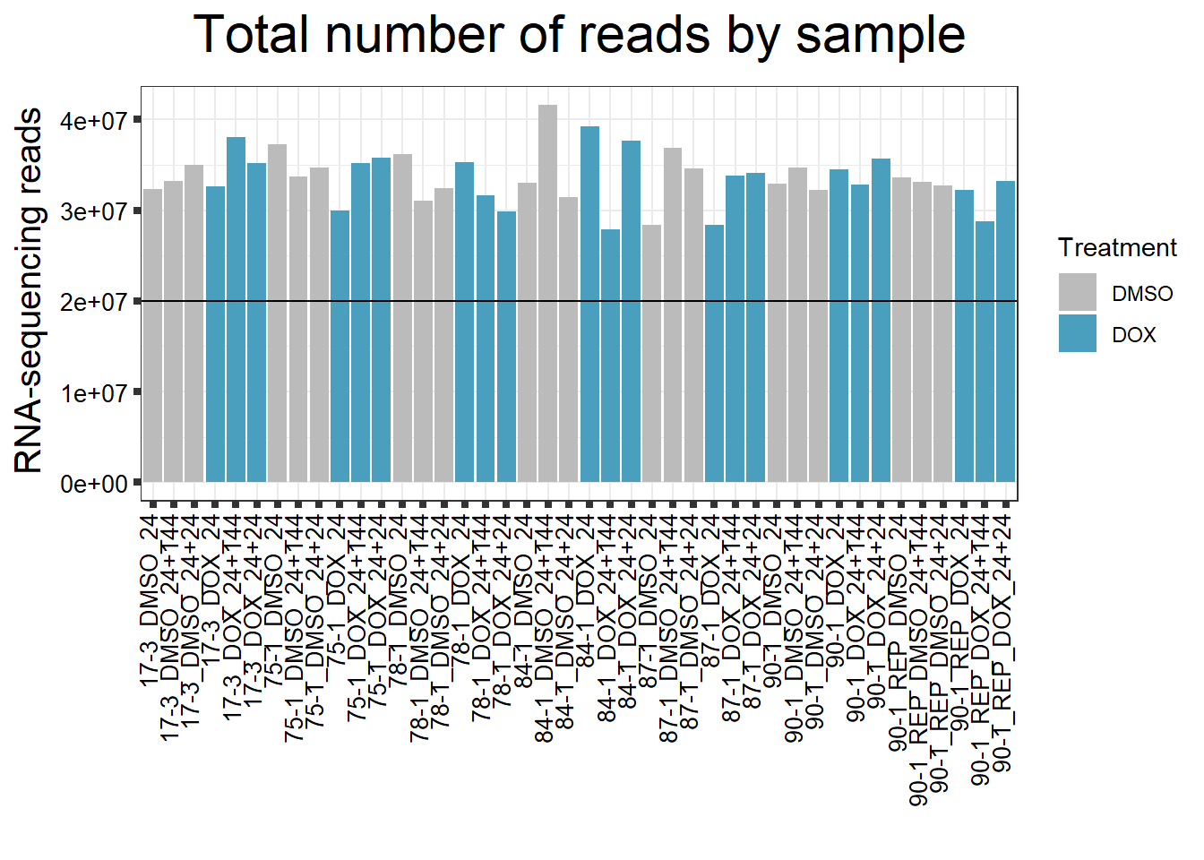
| Version | Author | Date |
|---|---|---|
| 29a5c35 | emmapfort | 2025-05-16 |
####Read Counts by Treatment####
fC_DOXCounts %>%
  ggplot(., aes (x =Treatment, y= Total_Align, fill = Treatment))+
  geom_boxplot()+
 scale_fill_manual(values=reads_by_sample)+
  ggtitle(expression("Total number of reads by treatment"))+
  xlab("")+
  ylab(expression("RNA-sequencing reads"))+
  theme_bw()+

  theme(plot.title = element_text(size = rel(2), hjust = 0.5),
        axis.title = element_text(size = 15, color = "black"),
        axis.ticks = element_line(linewidth = 1.5),
        axis.text.y = element_text(size =10, color = "black", angle = 0, hjust = 0.8, vjust = 0.5),
        axis.text.x = element_text(size =10, color = "black", angle = 90, hjust = 1, vjust = 0.2),
        #strip.text.x = element_text(size = 15, color = "black", face = "bold"),
        strip.text.y = element_text(color = "white"))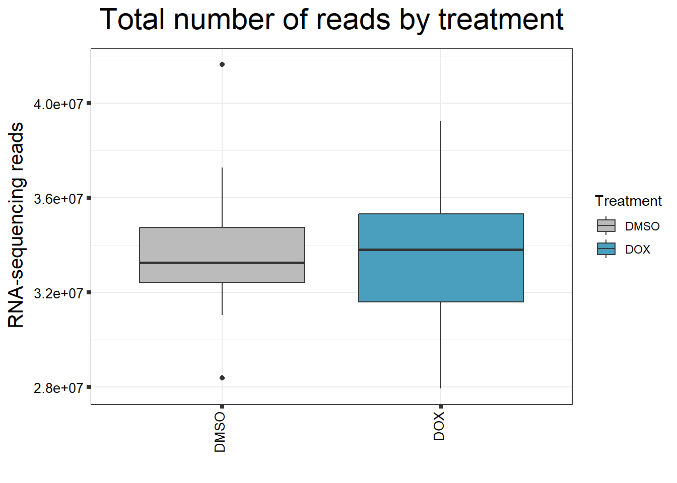
| Version | Author | Date |
|---|---|---|
| 29a5c35 | emmapfort | 2025-05-16 |
####Total Reads Per Individual####
fC_DOXCounts %>%
  ggplot(., aes (x =as.factor(Line), y=Total_Align))+
  geom_boxplot(aes(fill=as.factor(Line)))+
 scale_fill_brewer(palette = "Dark2", name = "Individual")+
  ggtitle(expression("Total number of reads by individual"))+
  xlab("")+
  ylab(expression("RNA-sequencing reads"))+
  theme_bw()+

  theme(plot.title = element_text(size = rel(2), hjust = 0.5),
        axis.title = element_text(size = 15, color = "black"),
        axis.ticks = element_line(linewidth = 1.5),
        axis.text.y = element_text(size =10, color = "black", angle = 0, hjust = 0.8, vjust = 0.5),
        axis.text.x = element_text(size =10, color = "black", angle = 0, hjust = 1),
        #strip.text.x = element_text(size = 15, color = "black", face = "bold"),
        strip.text.y = element_text(color = "white"))
| Version | Author | Date |
|---|---|---|
| 29a5c35 | emmapfort | 2025-05-16 |
####Total Mapped Reads Per Drug####

reads_by_sample <- c("DOX" = "#499FBD", "DMSO" = "#BBBBBC")
fC_DOXCounts %>%
  ggplot(., aes (x = Conditions, y = Assigned_Align, fill = Treatment, group_by = Line))+
  geom_col()+
 geom_hline(aes(yintercept=20000000))+
 scale_fill_manual(values=reads_by_sample)+
  ggtitle(expression("Total number of mapped reads by sample"))+
  xlab("")+
  ylab(expression("RNA-sequencing reads"))+
  theme_bw()+
  theme(plot.title = element_text(size = rel(2), hjust = 0.5),
        axis.title = element_text(size = 15, color = "black"),
        axis.ticks = element_line(linewidth = 1.5),
        axis.text.y = element_text(size =10, color = "black", angle = 0, hjust = 0.8, vjust = 0.5),
        axis.text.x = element_text(size =10, color = "black", angle = 90, hjust = 1, vjust = 0.2),
        #strip.text.x = element_text(size = 15, color = "black", face = "bold"),
        strip.text.y = element_text(color = "white"))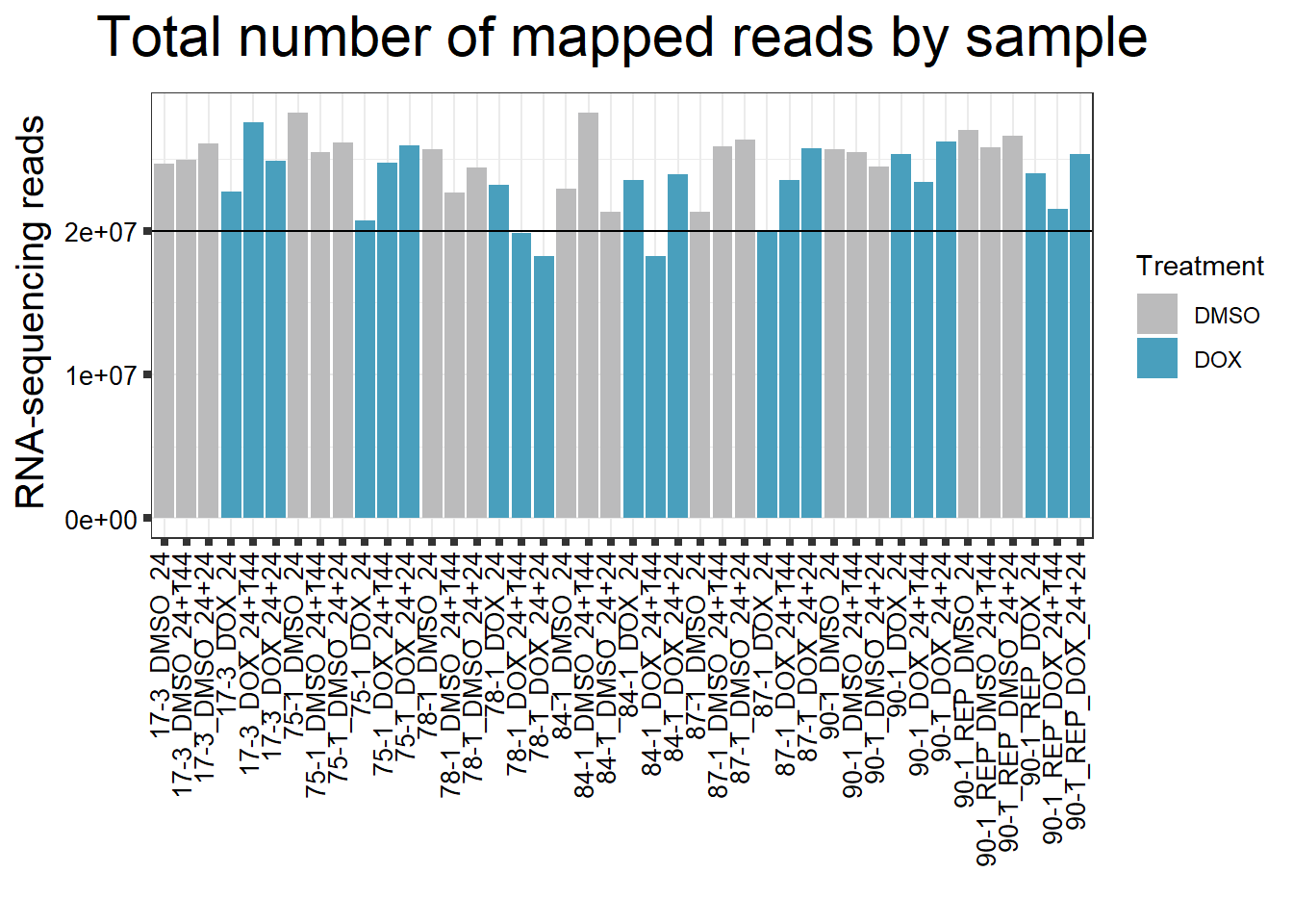
| Version | Author | Date |
|---|---|---|
| 29a5c35 | emmapfort | 2025-05-16 |
####Read Counts by Treatment####
fC_DOXCounts %>%
  ggplot(., aes (x =Treatment, y= Assigned_Align, fill = Treatment))+
  geom_boxplot()+
 scale_fill_manual(values=reads_by_sample)+
  ggtitle(expression("Total number of mapped reads by treatment"))+
  xlab("")+
  ylab(expression("RNA-sequencing reads"))+
  theme_bw()+

  theme(plot.title = element_text(size = rel(2), hjust = 0.5),
        axis.title = element_text(size = 15, color = "black"),
        axis.ticks = element_line(linewidth = 1.5),
        axis.text.y = element_text(size =10, color = "black", angle = 0, hjust = 0.8, vjust = 0.5),
        axis.text.x = element_text(size =10, color = "black", angle = 90, hjust = 1, vjust = 0.2),
        #strip.text.x = element_text(size = 15, color = "black", face = "bold"),
        strip.text.y = element_text(color = "white"))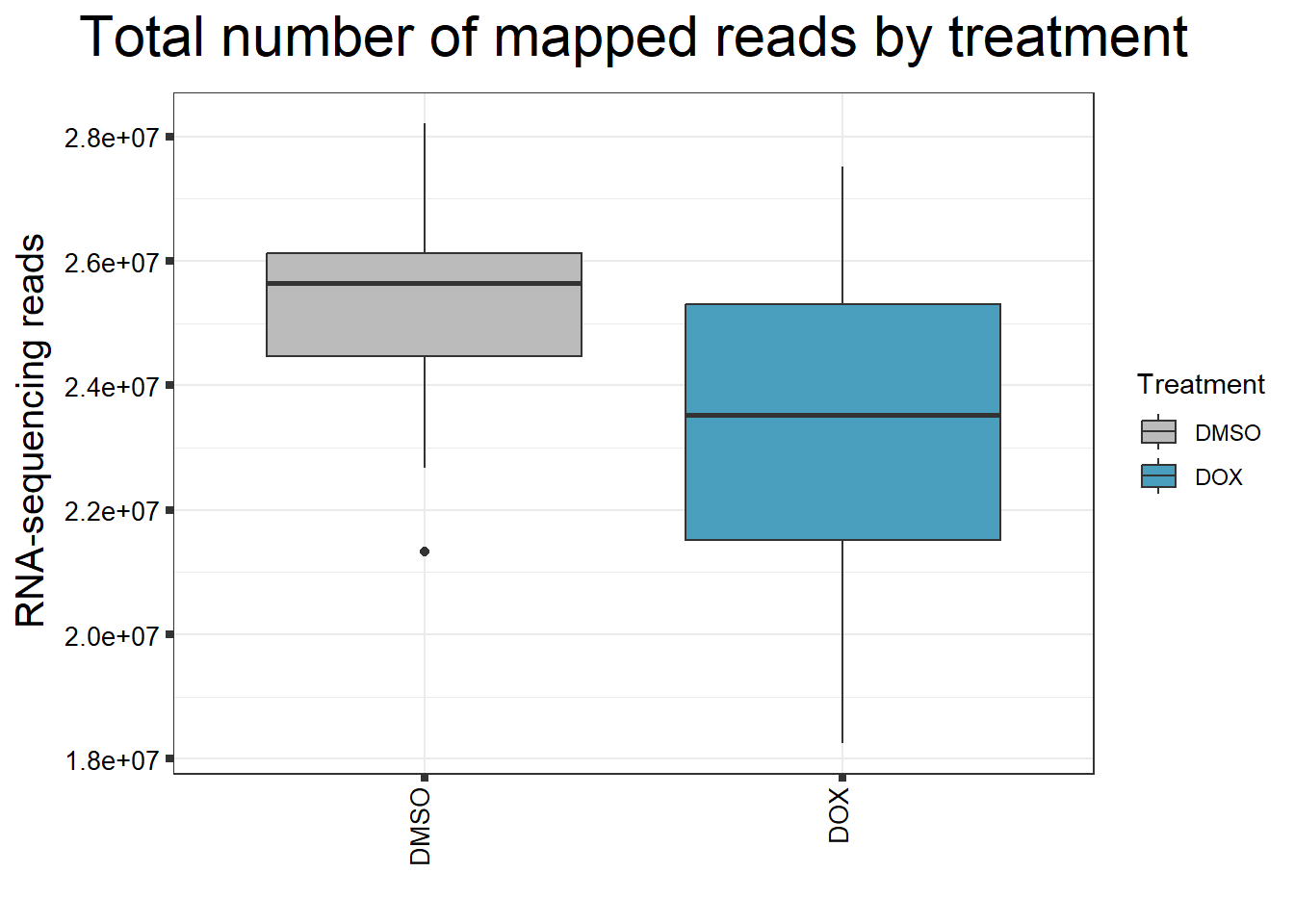
| Version | Author | Date |
|---|---|---|
| 29a5c35 | emmapfort | 2025-05-16 |
####Total Reads Per Individual####
fC_DOXCounts %>%
  ggplot(., aes (x =as.factor(Line), y=Assigned_Align))+
  geom_boxplot(aes(fill=as.factor(Line)))+
 scale_fill_brewer(palette = "Dark2", name = "Individual")+
  ggtitle(expression("Total number of mapped reads by individual"))+
  xlab("")+
  ylab(expression("RNA-sequencing reads"))+
  theme_bw()+

  theme(plot.title = element_text(size = rel(2), hjust = 0.5),
        axis.title = element_text(size = 15, color = "black"),
        axis.ticks = element_line(linewidth = 1.5),
        axis.text.y = element_text(size =10, color = "black", angle = 0, hjust = 0.8, vjust = 0.5),
        axis.text.x = element_text(size =10, color = "black", angle = 0, hjust = 1),
        #strip.text.x = element_text(size = 15, color = "black", face = "bold"),
        strip.text.y = element_text(color = "white"))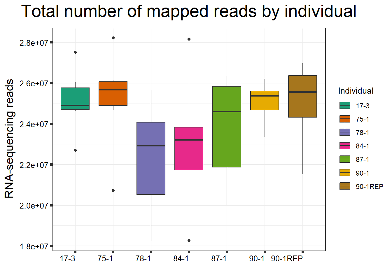
| Version | Author | Date |
|---|---|---|
| 29a5c35 | emmapfort | 2025-05-16 |
Now, I want to filter my dataframe Before I can filter by rowMeans, I must convert to log2cpm
#transform counts to cpm as a first step
counts_cpm_unfilt <- cpm(counts_raw_matrix, log = TRUE)
dim(counts_cpm_unfilt)
[1] 28395 42#I should have 28395 genes here since this is unfiltered
hist(counts_cpm_unfilt,
main = "Histogram of Unfiltered Counts",
xlab = expression("Log"[2]*" counts-per-million"),
col = 4)
| Version | Author | Date |
|---|---|---|
| 29a5c35 | emmapfort | 2025-05-16 |
###filter my data by rowMeans > 0 to exclude lowly expressed genes

filcpm_matrix <- subset(counts_cpm_unfilt, (rowMeans(counts_cpm_unfilt) > 0))
dim(filcpm_matrix)
[1] 14319 42#I should have 14319 genes here
#now let's make a histogram of this to check the difference
hist(filcpm_matrix,
main = "Histogram of Filtered Counts by rowMeans > 0",
xlab = expression("Log"[2]*" counts-per-million"),
col = 2)
| Version | Author | Date |
|---|---|---|
| 29a5c35 | emmapfort | 2025-05-16 |
#change the column names to match my samples - make sure that they are in the right order
#Individual 1 = 84-1 (M)
#Individual 2 = 87-1 (F)
#Individual 3 = 78-1 (F)
#Individual 4 = 75-1 (F)
#Individual 5 = 17-3 (M)
#Individual 6 = 90-1 (M)
#Individual 6REP = 90-1REP (M)

#Treatment/time should follow this order:
#DOX24tx
#DMSO24tx
#DOX24rec
#DMSO24rec
#DOX144rec
#DMSO144rec

colnames(filcpm_matrix) <- c("DOX_24T_Ind1",
                                "DMSO_24T_Ind1",
                                "DOX_24R_Ind1",
                                "DMSO_24R_Ind1",
                                "DOX_144R_Ind1",
                                "DMSO_144R_Ind1",
                                "DOX_24T_Ind2",
                                "DMSO_24T_Ind2",
                                "DOX_24R_Ind2",
                                "DMSO_24R_Ind2",
                                "DOX_144R_Ind2",
                                "DMSO_144R_Ind2",
                                "DOX_24T_Ind3",
                                "DMSO_24T_Ind3",
                                "DOX_24R_Ind3",
                                "DMSO_24R_Ind3",
                                "DOX_144R_Ind3",
                                "DMSO_144R_Ind3",
                                "DOX_24T_Ind4",
                                "DMSO_24T_Ind4",
                                "DOX_24R_Ind4",
                                "DMSO_24R_Ind4",
                                "DOX_144R_Ind4",
                                "DMSO_144R_Ind4",
                                "DOX_24T_Ind5",
                                "DMSO_24T_Ind5",
                                "DOX_24R_Ind5",
                                "DMSO_24R_Ind5",
                                "DOX_144R_Ind5",
                                "DMSO_144R_Ind5",
                                "DOX_24T_Ind6",
                                "DMSO_24T_Ind6",
                                "DOX_24R_Ind6",
                                "DMSO_24R_Ind6",
                                "DOX_144R_Ind6",
                                "DMSO_144R_Ind6",
                                "DOX_24T_Ind6REP",
                                "DMSO_24T_Ind6REP",
                                "DOX_24R_Ind6REP",
                                "DMSO_24R_Ind6REP",
                                "DOX_144R_Ind6REP",
                                "DMSO_144R_Ind6REP")

#export this as a csv
#write.csv(filcpm_matrix, "data/new/filcpm_final_matrix.csv")
#make boxplots of all counts vs log2cpm filtered counts
#set the margins so the x axis isn't cut off
##I don't mind if this one is partially cut off since all you need is the library number and not the whole name
par(mar = c(8,4,2,2))
#boxplot of unfiltered cpm matrix
boxplot(counts_cpm_unfilt,
main = "Boxplots of Unfiltered log2cpm",
names = colnames(counts_cpm_unfilt),
adj=1, las = 2, cex.axis = 0.7)
| Version | Author | Date |
|---|---|---|
| 29a5c35 | emmapfort | 2025-05-16 |
#set the margins so the x axis isn't cut off
par(mar = c(8,4,2,2))
#boxplot of filtered cpm matrix
boxplot(filcpm_matrix,
        main = "Boxplots of Filtered log2cpm (rowMeans > 0)",
        names = colnames(filcpm_matrix),
        adj=1, las = 2, cex.axis = 0.7)
| Version | Author | Date |
|---|---|---|
| 29a5c35 | emmapfort | 2025-05-16 |
After making my final matrix, I pulled the gene symbols from the entrez IDs I had as my rownames I ran this initially and then moved the column into my final matrix My final matrix is called filcpm_final_matrix.csv saved under data
##I did this earlier so don't run again, I put the list into the filcpm_final_matrix.csv
# # ----------------- Load Required Libraries -----------------
# library(dplyr)
# library(readr)
# library(org.Hs.eg.db)
# library(AnnotationDbi)
# # ----------------- Load Data -----------------
# sample_data <- read_csv("data/filcpm_final_matrix.csv", show_col_types = FALSE)
# # ----------------- Ensure Entrez_ID is Present and in Character Format -----------------
# # Check column names
# print(colnames(sample_data))
# # Rename if needed (adjust if the column name is not exactly 'Entrez_ID')
# # sample_data <- sample_data %>% rename(Entrez_ID = `actual_column_name`)
# # Convert Entrez_ID to character
# sample_data <- sample_data %>%
# mutate(Entrez_ID = as.character(Entrez_ID))
# # ----------------- Map Entrez_ID to Gene Symbol -----------------
# gene_symbols <- AnnotationDbi::select(
# org.Hs.eg.db,
# keys = sample_data$Entrez_ID,
# columns = c("SYMBOL"),
# keytype = "ENTREZID"
# )
# # ----------------- Join Back to Main Data -----------------
# sample_annotated <- left_join(sample_data, gene_symbols, by = c("Entrez_ID" = "ENTREZID"))
# # ----------------- Save Annotated Output -----------------
# #write_csv(sample_annotated, "data/Sample_annotated.csv")
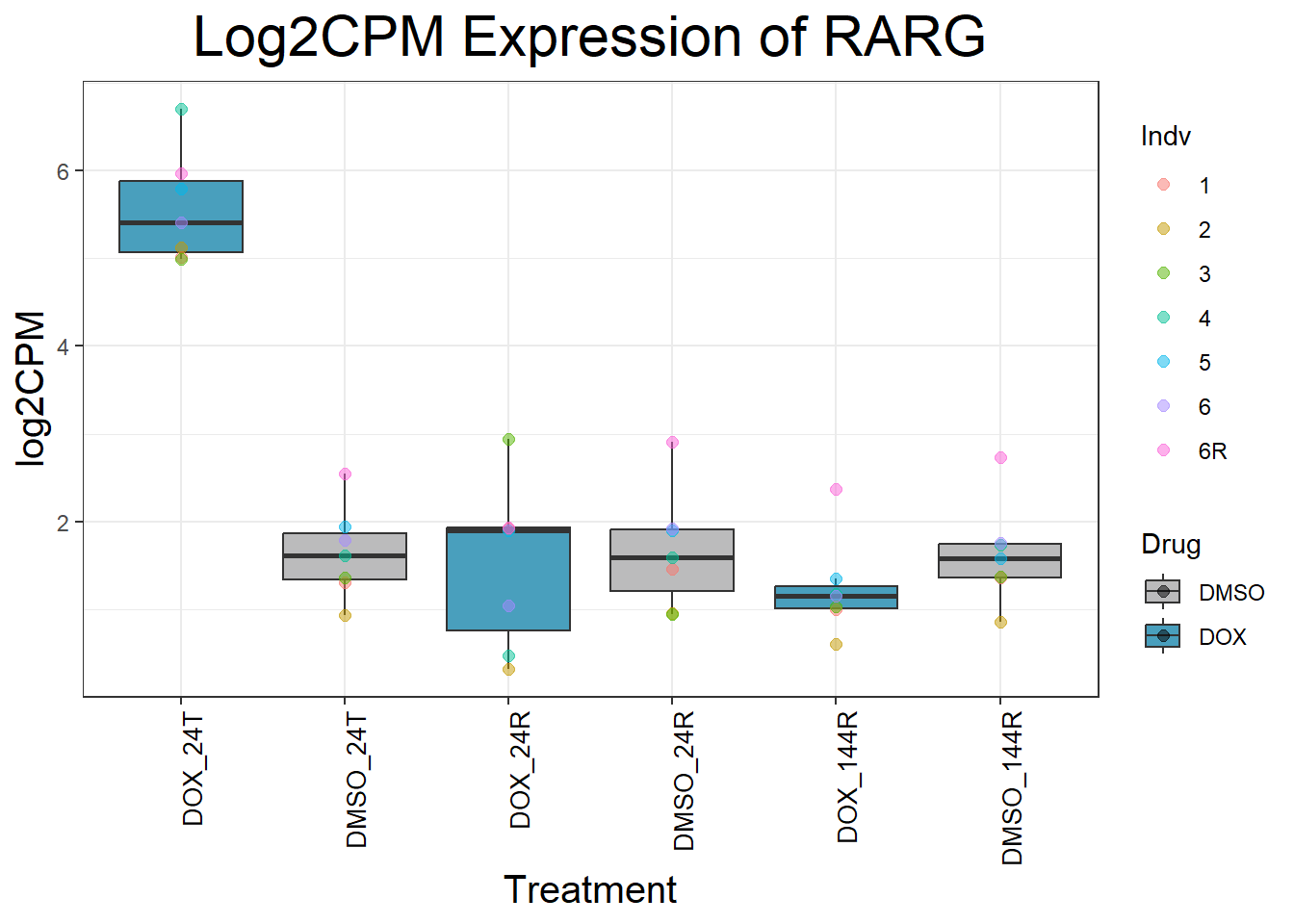
#Since I ran this before, Sample_annotated.csv columns of EntrezID and Symbol have been copied into my final matrix - so disregard this file except for record-keepingNow that I have my final matrix, I would like to check some key genes I want to make sure that these genes are responding as we expect We have triple checked this dataset to ensure that columns are in order
#Load in my count matrix
boxplot1 <- read.csv("data/new/filcpm_final_matrix.csv") %>%
as.data.frame()
#save boxplot1 as an object filcpm_matrix_genes
#saveRDS(boxplot1, "data/new/filcpm_matrix_genes.RDS")
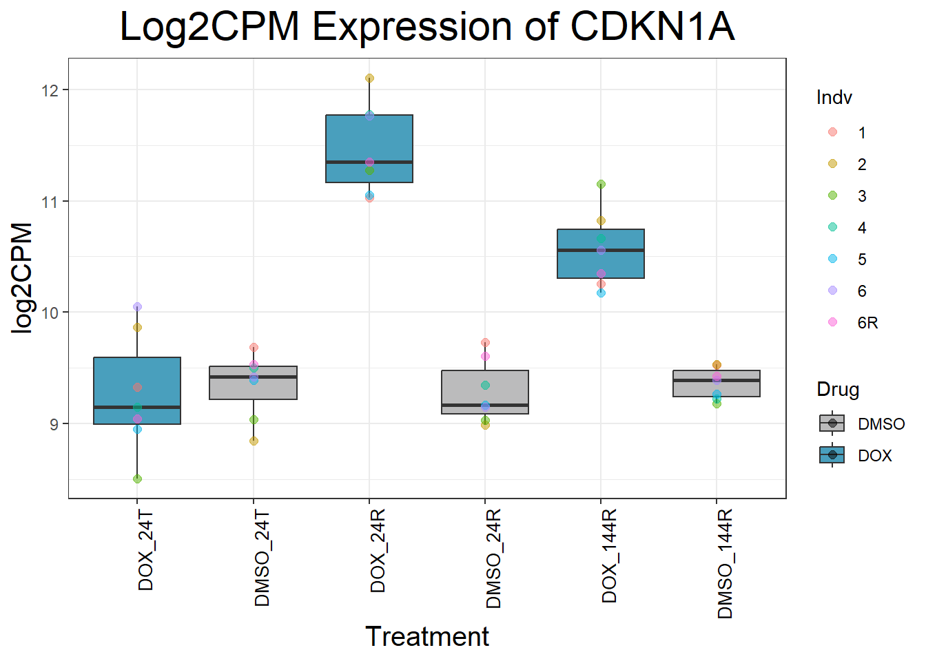
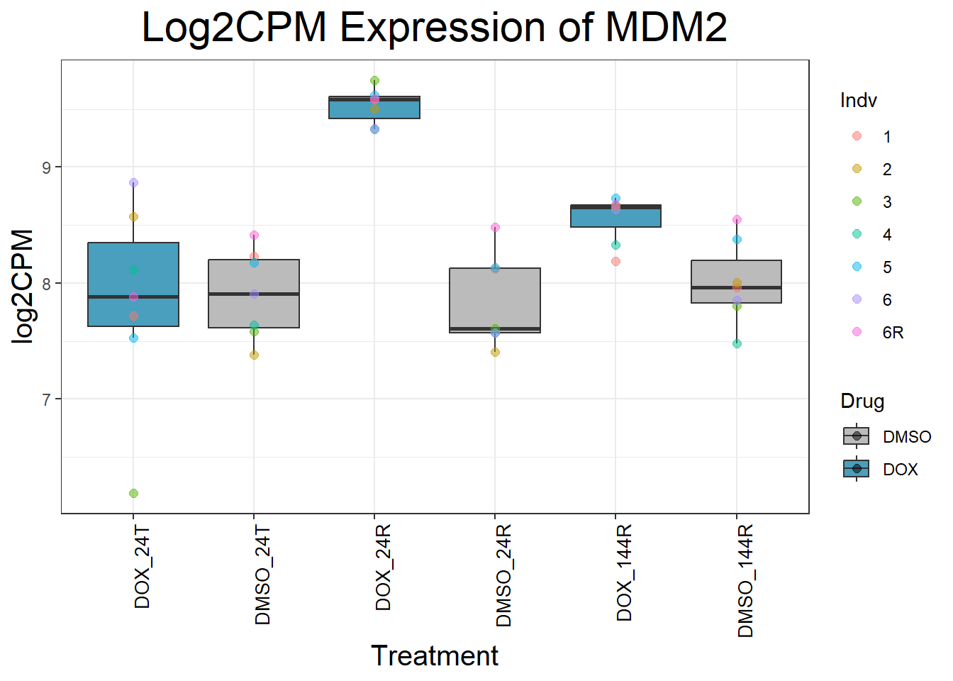
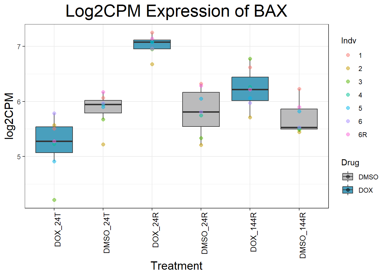
#Define gene list(s)
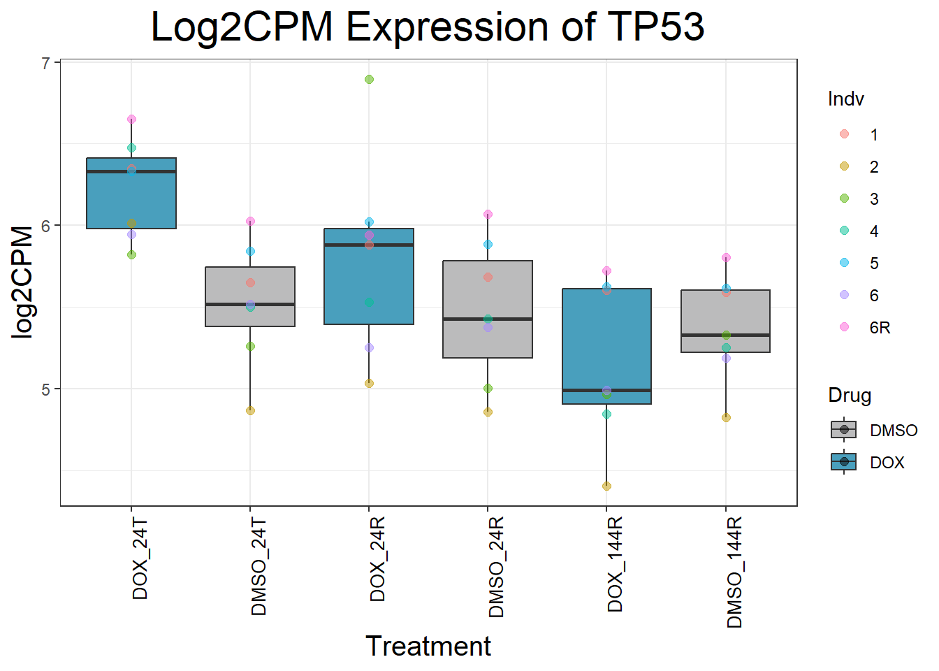
initial_test_genes <- c("CDKN1A", "MDM2", "BAX", "RARG", "TP53")
#Add more gene symbols as needed or add more categories
#Now put in the function I want to use to generate boxplots of genes
process_gene_data <- function(gene) {
gene_data <- boxplot1 %>% filter(SYMBOL == gene)
long_data <- gene_data %>%
pivot_longer(cols = -c(Entrez_ID, SYMBOL), names_to = "Sample", values_to = "log2CPM") %>%
mutate(
Drug = case_when(
grepl("DOX", Sample) ~ "DOX",
grepl("DMSO", Sample) ~ "DMSO",
TRUE ~ NA_character_
),
Timepoint = case_when(
grepl("_24T_", Sample) ~ "24T",
grepl("_24R_", Sample) ~ "24R",
grepl("_144R_", Sample) ~ "144R",
TRUE ~ NA_character_
),
Indv = case_when(
grepl("Ind1$", Sample) ~ "1",
grepl("Ind2$", Sample) ~ "2",
grepl("Ind3$", Sample) ~ "3",
grepl("Ind4$", Sample) ~ "4",
grepl("Ind5$", Sample) ~ "5",
grepl("Ind6$", Sample) ~ "6",
grepl("Ind6REP$", Sample) ~ "6R",
TRUE ~ NA_character_
),
Condition = paste(Drug, Timepoint, sep = "_")
)
long_data$Condition <- factor(
long_data$Condition,
levels = c(
"DOX_24T",
"DMSO_24T",
"DOX_24R",
"DMSO_24R",
"DOX_144R",
"DMSO_144R"
)
)
return(long_data)
}
#this function is saved under process_gene_data so I will save as an R object
#saveRDS(process_gene_data, "data/new/process_gene_data_funct.RDS")
#Generate Boxplots from the above function using our gene list above
for (gene in initial_test_genes) {
gene_data <- process_gene_data(gene)
p <- ggplot(gene_data, aes(x = Condition, y = log2CPM, fill = Drug)) +
geom_boxplot(outlier.shape = NA) +
geom_point(aes(color = Indv), size = 2, alpha = 0.5, position = position_jitter(width = -1, height = 0)) +
scale_fill_manual(values = c("DOX" = "#499FBD", "DMSO" = "#BBBBBC")) +
ggtitle(paste("Log2CPM Expression of", gene)) +
labs(x = "Treatment", y = "log2CPM") +
theme_bw() +
theme(
plot.title = element_text(size = rel(2), hjust = 0.5),
axis.title = element_text(size = 15, color = "black"),
axis.text.x = element_text(size = 10, color = "black", angle = 90, hjust = 1)
)
print(p)
}
| Version | Author | Date |
|---|---|---|
| 29a5c35 | emmapfort | 2025-05-16 |
| Version | Author | Date |
|---|---|---|
| 29a5c35 | emmapfort | 2025-05-16 |
| Version | Author | Date |
|---|---|---|
| 29a5c35 | emmapfort | 2025-05-16 |
| Version | Author | Date |
|---|---|---|
| 29a5c35 | emmapfort | 2025-05-16 |
| Version | Author | Date |
|---|---|---|
| 29a5c35 | emmapfort | 2025-05-16 |
Now I’ve confirmed with some boxplots that my genes are present and (mostly) behaving as they should - Sayan’s CDKN1A and MDM2 are initially high at 24hr in DOX 0.5 - My CDKN1A and MDM2 are similar to DMSO at 24hr DOX 0.5 - These genes increase at DOX24R - These genes are also high at DOX144R but not as high as 24R However, TP53 and BAX are acting similarly across our data
#Now I want to check if my data is as expected on a PCA plot
#perform PCA calculations
prcomp_res_unfilt <- prcomp(t(counts_cpm_unfilt %>% as.matrix()), center =  TRUE)

prcomp_res_filt <- prcomp(t(filcpm_matrix %>% as.matrix()), center =  TRUE)

#read in my metadata annotations
Metadata <- read.csv("data/new/Metadata.csv")

#add in labels for individual numbers
ind_num <- c("1", "1", "1", "1", "1", "1",
             "2", "2", "2", "2", "2", "2",
             "3", "3", "3", "3", "3", "3",
             "4", "4", "4", "4", "4", "4",
             "5", "5", "5", "5", "5", "5",
             "6", "6", "6", "6", "6", "6",
             "6R", "6R", "6R", "6R", "6R", "6R")

#now plot my PCA for unfiltered log2cpm
####PC1/PC2####
ggplot2::autoplot(prcomp_res_unfilt, data = Metadata, colour = "Condition", shape = "Time", size =4, x=1, y=2) +
  ggrepel::geom_text_repel(label=ind_num) +
  scale_color_manual(values=cond_col) +
  ggtitle(expression("PCA of Unfiltered log"[2]*"cpm")) +
  theme_bw()
Warning: ggrepel: 8 unlabeled data points (too many overlaps). Consider
increasing max.overlaps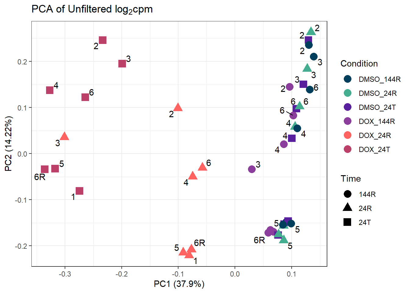
| Version | Author | Date |
|---|---|---|
| 29a5c35 | emmapfort | 2025-05-16 |
####PC2/PC3####
ggplot2::autoplot(prcomp_res_unfilt, data = Metadata, colour = "Condition", shape = "Time", size =4, x=2, y=3) +
  ggrepel::geom_text_repel(label=ind_num) +
  scale_color_manual(values=cond_col) +
  ggtitle(expression("PCA of Unfiltered log"[2]*"cpm")) +
  theme_bw()
Warning: ggrepel: 6 unlabeled data points (too many overlaps). Consider
increasing max.overlaps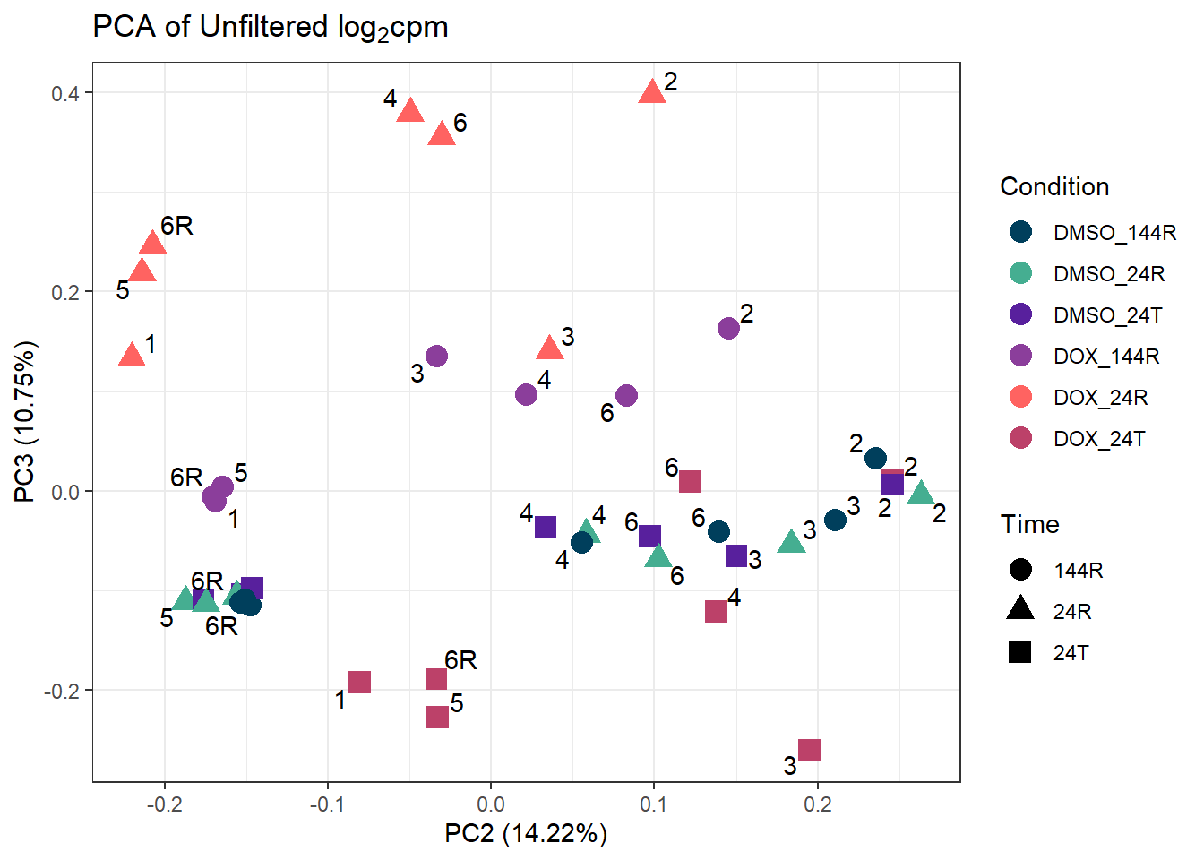
| Version | Author | Date |
|---|---|---|
| 29a5c35 | emmapfort | 2025-05-16 |
####PC3/PC4####
ggplot2::autoplot(prcomp_res_unfilt, data = Metadata, colour = "Condition", shape = "Time", size =4, x=3, y=4) +
  ggrepel::geom_text_repel(label=ind_num) +
  scale_color_manual(values=cond_col) +
  ggtitle(expression("PCA of Unfiltered log"[2]*"cpm")) +
  theme_bw()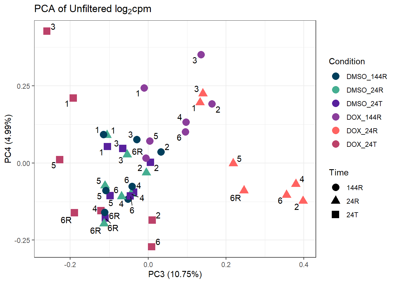
| Version | Author | Date |
|---|---|---|
| 29a5c35 | emmapfort | 2025-05-16 |
#Now plot my PCA for filtered log2cpm
####PC1/PC2####
ggplot2::autoplot(prcomp_res_filt, data = Metadata, colour = "Condition", shape = "Time", size =4, x=1, y=2) +
  ggrepel::geom_text_repel(label=ind_num) +
  scale_color_manual(values=cond_col) +
  ggtitle(expression("PCA of Filtered log"[2]*"cpm")) +
  theme_bw()
Warning: ggrepel: 7 unlabeled data points (too many overlaps). Consider
increasing max.overlaps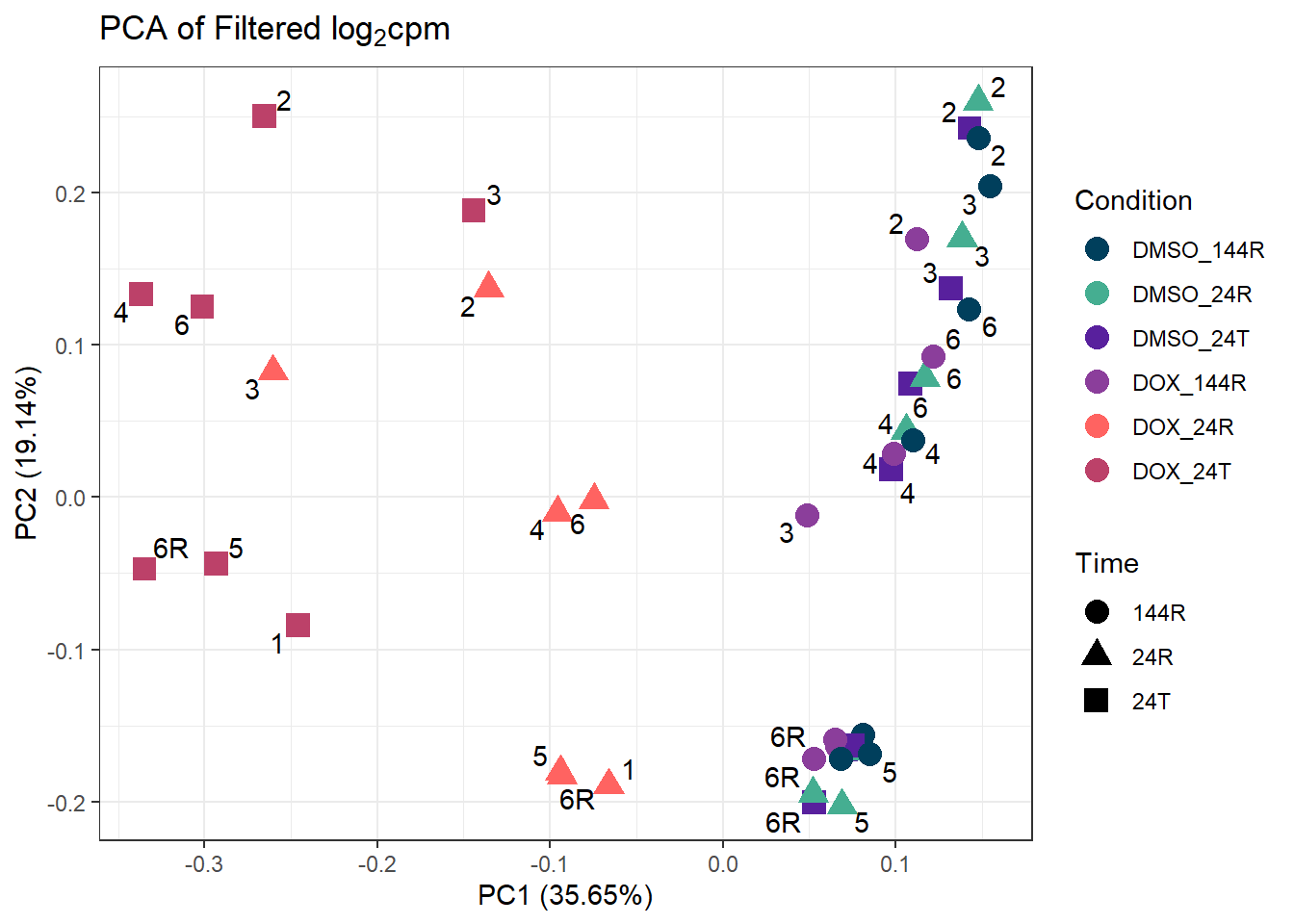
| Version | Author | Date |
|---|---|---|
| 29a5c35 | emmapfort | 2025-05-16 |
####PC2/PC3####
ggplot2::autoplot(prcomp_res_filt, data = Metadata, colour = "Condition", shape = "Time", size =4, x=2, y=3) +
  ggrepel::geom_text_repel(label=ind_num) +
  scale_color_manual(values=cond_col) +
  ggtitle(expression("PCA of Filtered log"[2]*"cpm")) +
  theme_bw()
Warning: ggrepel: 3 unlabeled data points (too many overlaps). Consider
increasing max.overlaps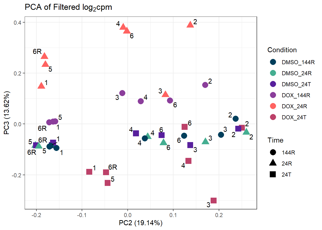
| Version | Author | Date |
|---|---|---|
| 29a5c35 | emmapfort | 2025-05-16 |
####PC3/PC4####
ggplot2::autoplot(prcomp_res_filt, data = Metadata, colour = "Condition", shape = "Time", size =4, x=3, y=4) +
  ggrepel::geom_text_repel(label=ind_num) +
  scale_color_manual(values=cond_col) +
  ggtitle(expression("PCA of Filtered log"[2]*"cpm")) +
  theme_bw()
Warning: ggrepel: 1 unlabeled data points (too many overlaps). Consider
increasing max.overlaps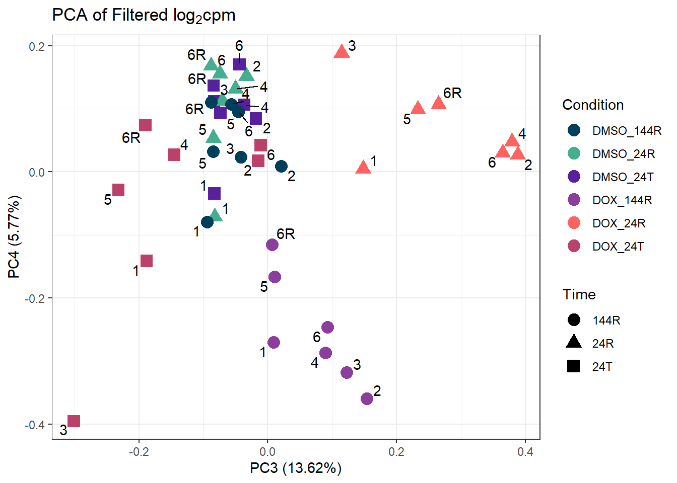
| Version | Author | Date |
|---|---|---|
| 29a5c35 | emmapfort | 2025-05-16 |
#check to make sure that the column names are correct
lcpm_2 <- filcpm_matrix
colnames(lcpm_2) <- Metadata$Final_sample_name

#compute the correlation matrices, one pearson and one spearman
cor_matrix_pearson <- cor(lcpm_2,
                          y = NULL,
                          use = "everything",
                          method = "pearson")
cor_matrix_spearman <- cor(lcpm_2,
                           y = NULL,
                           use = "everything",
                           method = "spearman")

# Extract metadata columns
Individual <- as.character(Metadata$Ind)
Time <- as.character(Metadata$Time)
Treatment <- as.character(Metadata$Drug)

# Define color palettes for annotations
annot_col_cor = list(drugs = c("DOX" = "#499FBD",
                               "DMSO" = "#BBBBBC"),
                     individuals = c("1" = "#003F5C",
                                     "2" = "#45AE91",
                                     "3" = "#58209D",
                                     "4" = "#8B3E9B",
                                     "5" = "#FF6361",
                                     "6" = "#BC4169",
                                     "6R" = "#FF2362"),
                     timepoints = c("24T" = "#238B45",
                                    "24R" = "#74C476",
                                    "144R" = "#C7E9C0"))

drug_colors <- c("DOX" = "#499FBD",
                 "DMSO" = "#BBBBBC")
ind_colors <- c("1" = "red",
                "2" = "orange",
                "3" = "yellow",
                "4" = "green",
                "5" = "blue",
                "6" = "violet",
                "6R" = "purple")
time_colors <- c("24T" = "#238B45",
                 "24R" = "#74C476",
                 "144R" = "#C7E9C0")

# Create annotations
top_annotation <- HeatmapAnnotation(
  Individual = Individual,
  Time = Time,
  Treatment = Treatment,
  col = list(
    Individual = ind_colors,
    Time = time_colors,
    Treatment = drug_colors
  )
)

####ANNOTATED HEATMAPS####
# pheatmap(cor_matrix_pearson, border_color = "black", legend = TRUE, angle_col = 90, display_numbers = FALSE, number_color = "black", fontsize = 10, fontsize_number = 5, annotation_col = top_annotation, annotation_colors = annot_col)

####Pearson Heatmap####
heatmap_pearson <- Heatmap(cor_matrix_pearson,
                           name = "Pearson",
                           top_annotation = top_annotation,
                           show_row_names = TRUE,
                           show_column_names = TRUE,
                           cluster_rows = TRUE,
                           cluster_columns = TRUE,
                           border = TRUE)

# Draw the heatmap
draw(heatmap_pearson)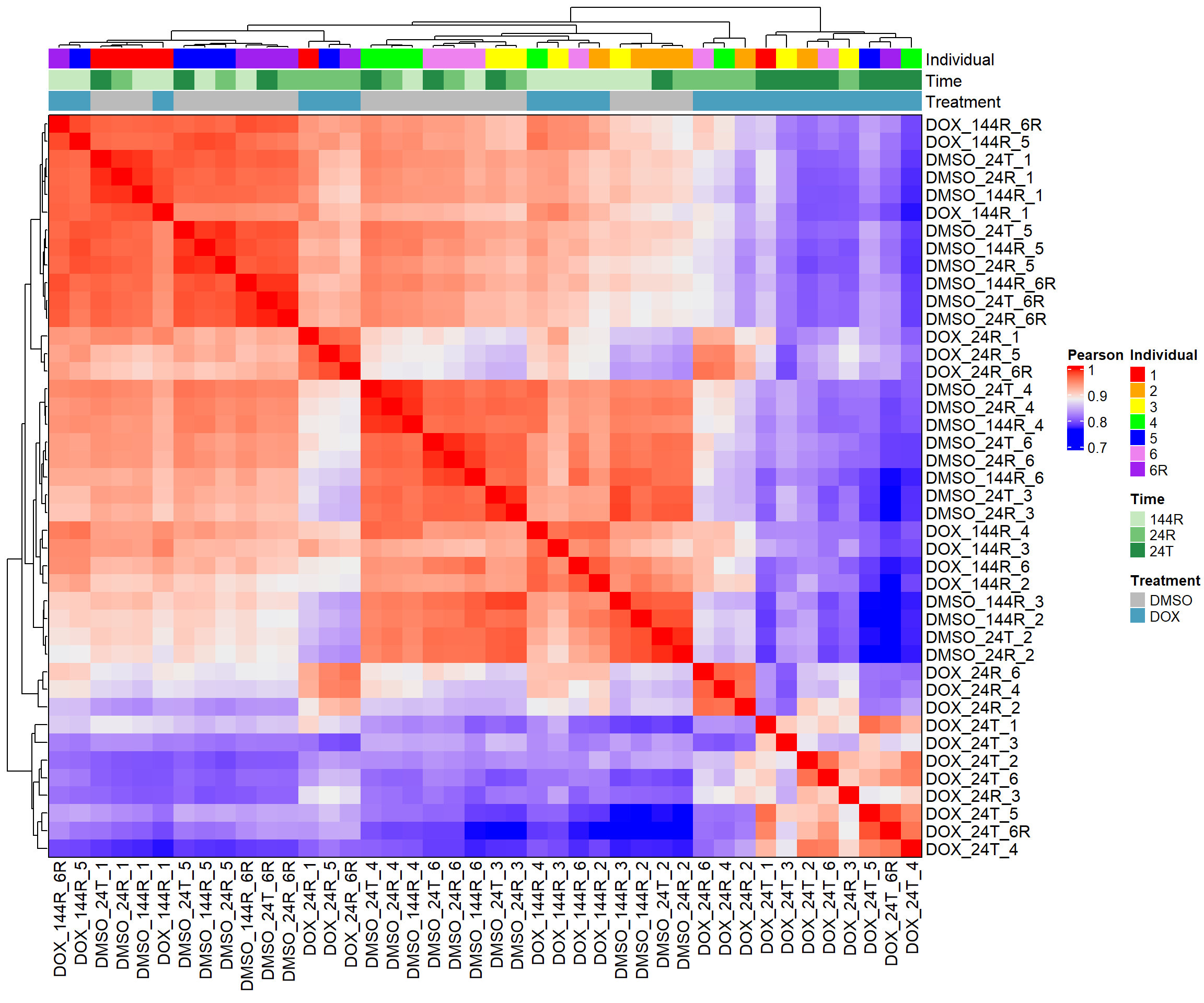
| Version | Author | Date |
|---|---|---|
| 29a5c35 | emmapfort | 2025-05-16 |
####Spearman Heatmap####
heatmap_spearman <- Heatmap(cor_matrix_spearman,
                           name = "Spearman",
                           top_annotation = top_annotation,
                           show_row_names = TRUE,
                           show_column_names = TRUE,
                           cluster_rows = TRUE,
                           cluster_columns = TRUE,
                           border = TRUE)

# Draw the heatmap
draw(heatmap_spearman)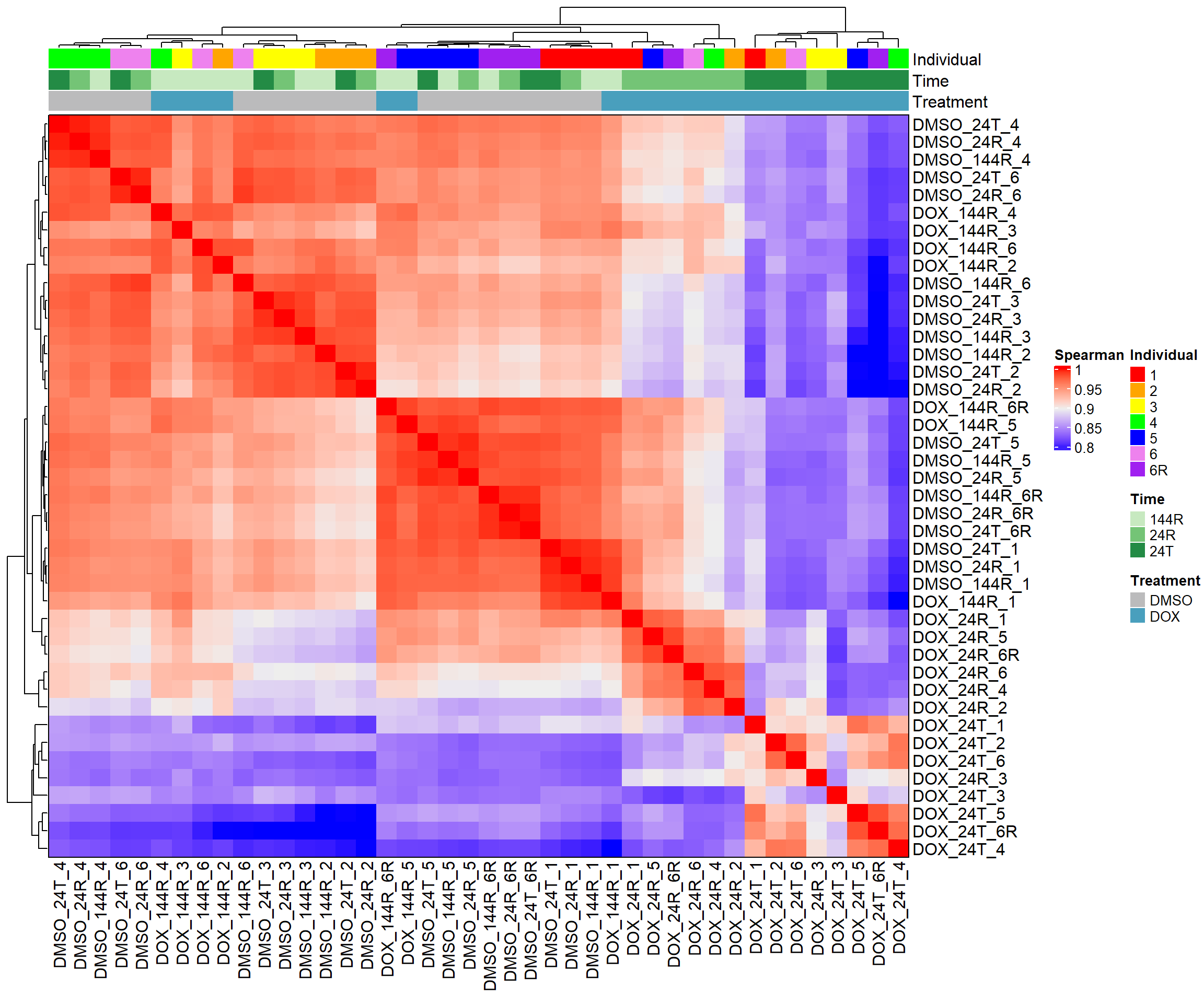
| Version | Author | Date |
|---|---|---|
| 29a5c35 | emmapfort | 2025-05-16 |
#Now I want to make a filtered gene list (my rownames)
##I will use this to filter my counts for limma + Cormotif

filt_gene_list <- rownames(filcpm_matrix)
#save this filtered gene list as I'll use it to filter my counts
#saveRDS(filt_gene_list, "data/new/filt_gene_list.RDS")
counts_raw_matrix <- readRDS("data/new/counts_raw_matrix.RDS")
#change column names to match samples for my raw counts matrix
colnames(counts_raw_matrix) <- c("DOX_24T_Ind1",
"DMSO_24T_Ind1",
"DOX_24R_Ind1",
"DMSO_24R_Ind1",
"DOX_144R_Ind1",
"DMSO_144R_Ind1",
"DOX_24T_Ind2",
"DMSO_24T_Ind2",
"DOX_24R_Ind2",
"DMSO_24R_Ind2",
"DOX_144R_Ind2",
"DMSO_144R_Ind2",
"DOX_24T_Ind3",
"DMSO_24T_Ind3",
"DOX_24R_Ind3",
"DMSO_24R_Ind3",
"DOX_144R_Ind3",
"DMSO_144R_Ind3",
"DOX_24T_Ind4",
"DMSO_24T_Ind4",
"DOX_24R_Ind4",
"DMSO_24R_Ind4",
"DOX_144R_Ind4",
"DMSO_144R_Ind4",
"DOX_24T_Ind5",
"DMSO_24T_Ind5",
"DOX_24R_Ind5",
"DMSO_24R_Ind5",
"DOX_144R_Ind5",
"DMSO_144R_Ind5",
"DOX_24T_Ind6",
"DMSO_24T_Ind6",
"DOX_24R_Ind6",
"DMSO_24R_Ind6",
"DOX_144R_Ind6",
"DMSO_144R_Ind6",
"DOX_24T_Ind6REP",
"DMSO_24T_Ind6REP",
"DOX_24R_Ind6REP",
"DMSO_24R_Ind6REP",
"DOX_144R_Ind6REP",
"DMSO_144R_Ind6REP")
#subset my count matrix based on filtered CPM matrix
x <- counts_raw_matrix[row.names(filcpm_matrix),]
dim(x)[1] 14319 42#14319 genes as expected!
#this is still in counts form
#remove my replicate individual at this time
x_norep <- x[,1:36]
#modify my metadata to match
Metadata_2 <- Metadata[1:36,]
rownames(Metadata_2) <- Metadata_2$Sample_bam
colnames(x_norep) <- Metadata_2$Sample_ID
rownames(Metadata_2) <- Metadata_2$Sample_ID
Metadata_2$Condition <- make.names(Metadata_2$Condition)
Metadata_2$Ind <- as.character(Metadata_2$Ind)#create DGEList object
dge <- DGEList(counts = x_norep)
dge$samples$group <- factor(Metadata_2$Condition)
dge <- calcNormFactors(dge, method = "TMM")
#saveRDS(dge, "data/new/dge_matrix.RDS")
#check normalization factors from TMM normalization of LIBRARIES
dge$samples group lib.size norm.factors
84-1_DOX_24 DOX_24T 23393931 0.9745263
84-1_DMSO_24 DMSO_24T 22853195 0.9565797
84-1_DOX_24+24 DOX_24R 23846995 1.1659432
84-1_DMSO_24+24 DMSO_24R 21299355 0.9649641
84-1_DOX_24+144 DOX_144R 18222568 0.9913625
84-1_DMSO_24+144 DMSO_144R 28115884 0.9653464
87-1_DOX_24 DOX_24T 19935097 1.0526605
87-1_DMSO_24 DMSO_24T 21302879 0.9773889
87-1_DOX_24+24 DOX_24R 25636959 1.0751043
87-1_DMSO_24+24 DMSO_24R 26319662 0.9940323
87-1_DOX_24+144 DOX_144R 23463426 0.9003102
87-1_DMSO_24+144 DMSO_144R 25840938 0.9888449
78-1_DOX_24 DOX_24T 23085807 0.7676077
78-1_DMSO_24 DMSO_24T 25610495 1.0077383
78-1_DOX_24+24 DOX_24R 18083930 1.1682704
78-1_DMSO_24+24 DMSO_24R 24331177 0.9906872
78-1_DOX_24+144 DOX_144R 19754391 0.9941834
78-1_DMSO_24+144 DMSO_144R 22641509 1.0010734
75-1_DOX_24 DOX_24T 20583626 1.0676786
75-1_DMSO_24 DMSO_24T 28166198 1.0031906
75-1_DOX_24+24 DOX_24R 25831427 1.1530208
75-1_DMSO_24+24 DMSO_24R 26081158 1.0058953
75-1_DOX_24+144 DOX_144R 24659898 0.9261599
75-1_DMSO_24+144 DMSO_144R 25412931 0.9703454
17-3_DOX_24 DOX_24T 22518848 0.9766893
17-3_DMSO_24 DMSO_24T 24589534 0.9612345
17-3_DOX_24+24 DOX_24R 24797547 1.1703079
17-3_DMSO_24+24 DMSO_24R 25977536 0.9509690
17-3_DOX_24+144 DOX_144R 27447106 0.9422729
17-3_DMSO_24+144 DMSO_144R 24893583 0.9356377
90-1_DOX_24 DOX_24T 25187428 1.0311957
90-1_DMSO_24 DMSO_24T 25630519 1.0283437
90-1_DOX_24+24 DOX_24R 26138399 1.1183471
90-1_DMSO_24+24 DMSO_24R 24430396 0.9988688
90-1_DOX_24+144 DOX_144R 23323463 0.9496884
90-1_DMSO_24+144 DMSO_144R 25424152 0.9872926#create my design matrix for DE
design <- model.matrix(~ 0 + Metadata_2$Condition)
colnames(design) <- gsub("Metadata_2\\$Condition", "", colnames(design))
#take care that the matrix automatically sorts cols alphabetically
##currently DMSO144R, DMSO24R, DMSO24T, DOX144R, DOX24R, DOX24T
#run duplicate correlation for individual effect
corfit <- duplicateCorrelation(object = dge$counts, design = design, block = Metadata_2$Ind)
#voom transformation and plot
v <- voom(dge, design, block = Metadata_2$Ind, correlation = corfit$consensus.correlation, plot = TRUE)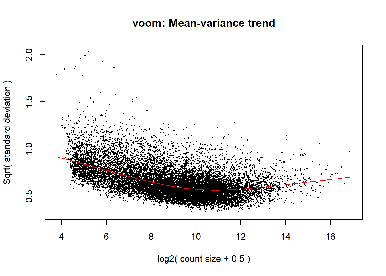
| Version | Author | Date |
|---|---|---|
| 29a5c35 | emmapfort | 2025-05-16 |
#fit my linear model
fit <- lmFit(v, design, block = Metadata_2$Ind, correlation = corfit$consensus.correlation)

#make my contrast matrix to compare across tx and veh
contrast_matrix <- makeContrasts(
  V.D24T = DOX_24T - DMSO_24T,
  V.D24R = DOX_24R - DMSO_24R,
  V.D144R = DOX_144R - DMSO_144R,
  levels = design
)

#apply these contrasts to compare DOX to DMSO VEH
fit2 <- contrasts.fit(fit, contrast_matrix)
fit2 <- eBayes(fit2)

#plot the mean-variance trend
plotSA(fit2, main = "Final model: Mean-Variance trend")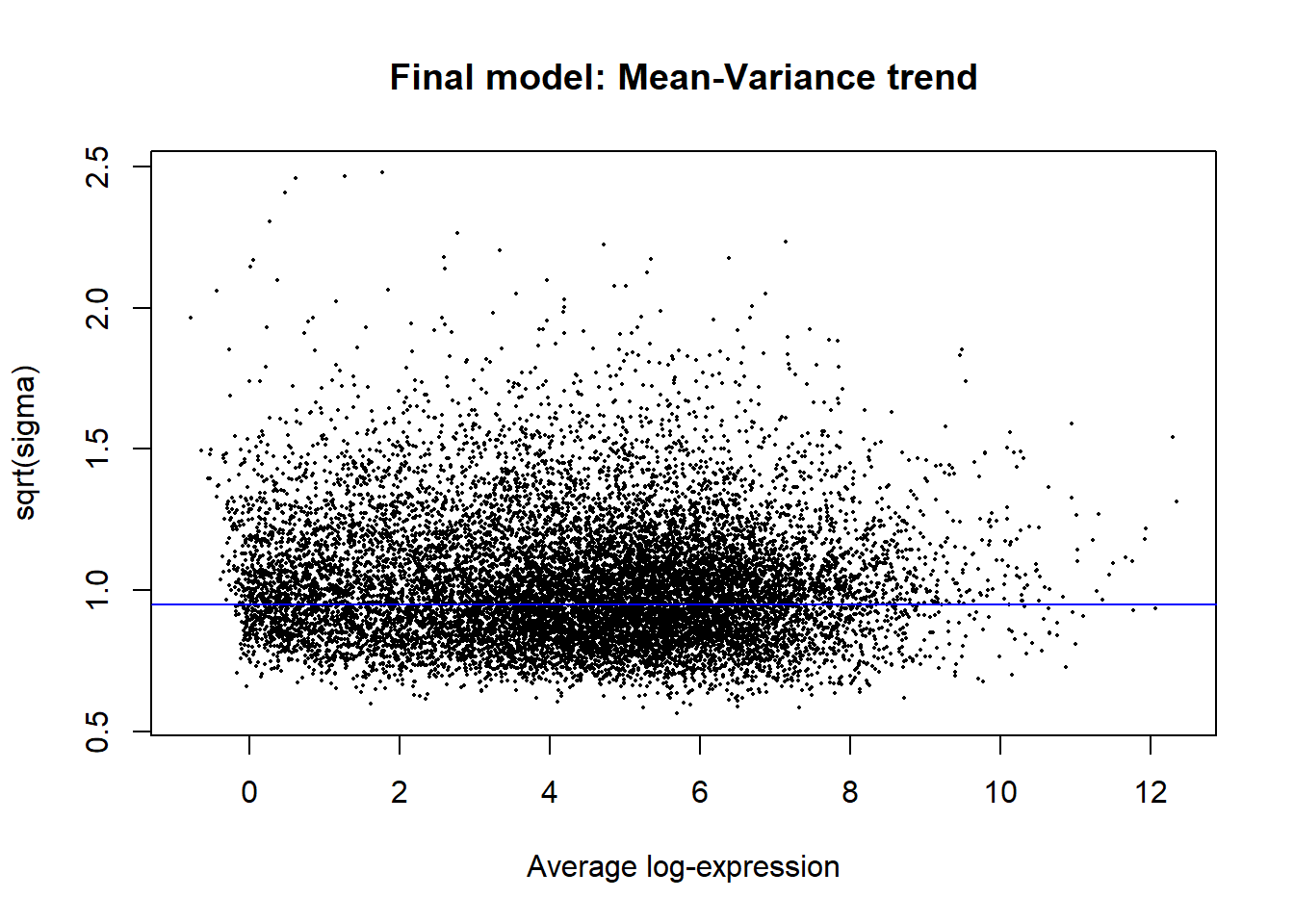
| Version | Author | Date |
|---|---|---|
| 29a5c35 | emmapfort | 2025-05-16 |
#look at the summary of your results
##this tells you the number of DEGs in each condition
results_summary <- decideTests(fit2, adjust.method = "BH", p.value = 0.05)
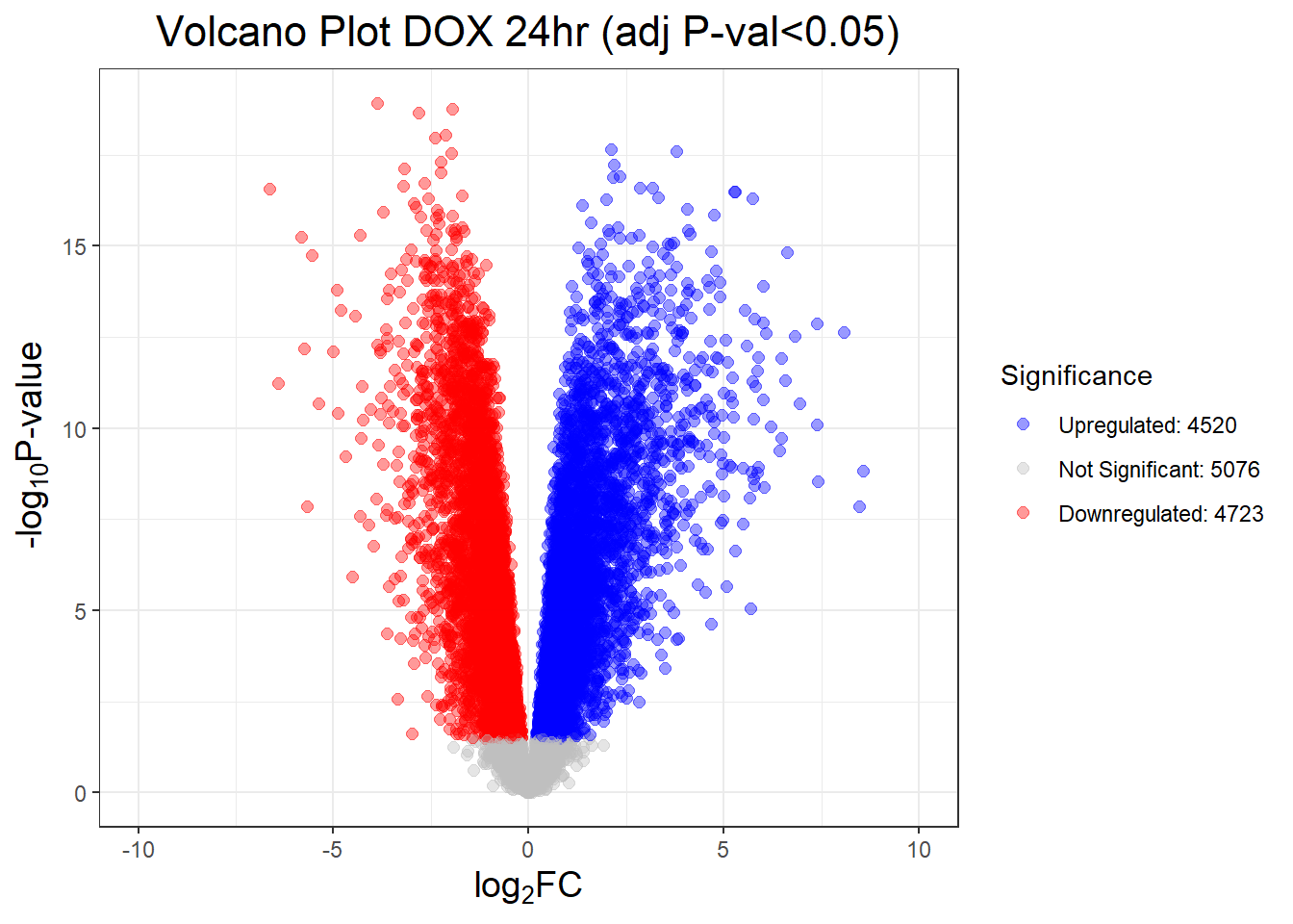
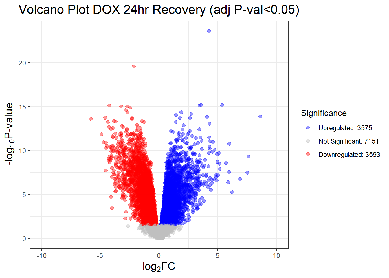
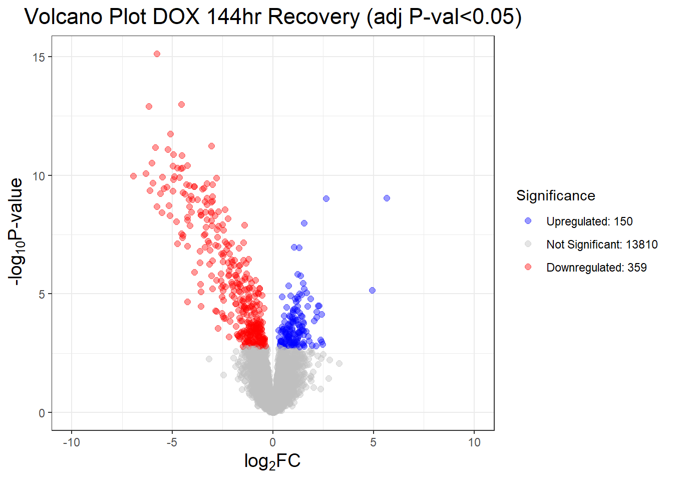
summary(results_summary) V.D24T V.D24R V.D144R
Down 4723 3593 359
NotSig 5076 7151 13810
Up 4520 3575 150# V.D24 V.D24r V.D144r
# Down 4723 3593 359
# NotSig 5076 7151 13810
# Up 4520 3575 150# Generate Top Table for Specific Comparisons
Toptable_V.D24T <- topTable(fit = fit2, coef = "V.D24T", number = nrow(x), adjust.method = "BH", p.value = 1, sort.by = "none")
#write.csv(Toptable_V.D24T, "data/new/DEGs/Toptable_V.D24T.csv")
Toptable_V.D24R <- topTable(fit = fit2, coef = "V.D24R", number = nrow(x), adjust.method = "BH", p.value = 1, sort.by = "none")
#write.csv(Toptable_V.D24R, "data/new/DEGs/Toptable_V.D24R.csv")
Toptable_V.D144R <- topTable(fit = fit2, coef = "V.D144R", number = nrow(x), adjust.method = "BH", p.value = 1, sort.by = "none")
#write.csv(Toptable_V.D144R, "data/new/DEGs/Toptable_V.D144R.csv")
#save all of these toptables as R objects
# saveRDS(list(
# V.D24T = Toptable_V.D24T,
# V.D24R = Toptable_V.D24R,
# V.D144R = Toptable_V.D144R
# ), file = "data/new/Toptable_list.RDS")
Toptable_list <- readRDS("data/new/Toptable_list.RDS")#make a function to generate volcano plots + add gene numbers
generate_volcano_plot <- function(toptable, title) {
#make significance labels
toptable$Significance <- "Not Significant"
toptable$Significance[toptable$logFC > 0 & toptable$adj.P.Val < 0.05] <- "Upregulated"
toptable$Significance[toptable$logFC < 0 & toptable$adj.P.Val < 0.05] <- "Downregulated"
#add number of genes for each significance label
upgenes <- toptable %>% filter(Significance == "Upregulated") %>% nrow()
nsgenes <- toptable %>% filter(Significance == "Not Significant") %>% nrow()
downgenes <- toptable %>% filter(Significance == "Downregulated") %>% nrow()
#make legend labels for no of genes
legend_lab <- c(
str_c("Upregulated: ", upgenes),
str_c("Not Significant: ", nsgenes),
str_c("Downregulated: ", downgenes)
)
#specify the colors for the legend
legend_col <- c(
str_c("Upregulated: " = "blue"),
str_c("Not Significant: " = "gray"),
str_c("Downregulated: " = "red")
)
#generate volcano plot w/ legend
ggplot(toptable, aes(x = logFC,
y = -log10(P.Value),
color = Significance)) +
geom_point(alpha = 0.4, size = 2) +
scale_color_manual(values = c("Upregulated" = "blue",
"Not Significant" = "gray",
"Downregulated" = "red"),
labels = legend_lab) +
xlim(-10, 10) +
labs(title = title,
x = expression(x = "log"[2]*"FC"),
y = expression(y = "-log"[10]*"P-value")) +
theme_bw()+
guides(color = guide_legend(override.aes = list(color = legend_col)))+
theme(legend.position = "right",
plot.title = element_text(size = rel(1.5), hjust = 0.5),
axis.title = element_text(size = rel(1.25)))
}
#generate volcano plots across each comparison
volcano_plots <- list(
"V.D24T" = generate_volcano_plot(Toptable_V.D24T, "Volcano Plot DOX 24hr (adj P-val<0.05)"),
"V.D24R" = generate_volcano_plot(Toptable_V.D24R, "Volcano Plot DOX 24hr Recovery (adj P-val<0.05)"),
"V.D144R" = generate_volcano_plot(Toptable_V.D144R, "Volcano Plot DOX 144hr Recovery (adj P-val<0.05)")
)
# Display each volcano plot
for (plot_name in names(volcano_plots)) {
print(volcano_plots[[plot_name]])
}
| Version | Author | Date |
|---|---|---|
| 29a5c35 | emmapfort | 2025-05-16 |
| Version | Author | Date |
|---|---|---|
| 29a5c35 | emmapfort | 2025-05-16 |
| Version | Author | Date |
|---|---|---|
| 29a5c35 | emmapfort | 2025-05-16 |
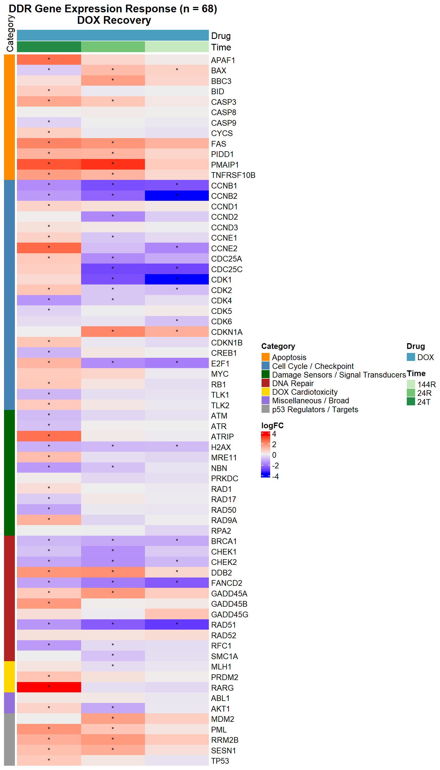
#DDR Gene Expression Heatmap — DOX Over Recovery Time (68 genes, with categories)

# Load libraries
# library(circlize)
# library(grid)
# library(reshape2)

# Load DEG files
load_deg <- function(path) read.csv(path)

DOX_24T <- load_deg("data/new/DEGs/Toptable_V.D24T.csv")
DOX_24R <- load_deg("data/new/DEGs/Toptable_V.D24R.csv")
DOX_144R <- load_deg("data/new/DEGs/Toptable_V.D144R.csv")

# Final Entrez IDs and categories (68 genes)
entrez_category <- tribble(
  ~ENTREZID, ~Category,
  317, "Apoptosis", 355, "Apoptosis", 581, "Apoptosis", 637, "Apoptosis",
  836, "Apoptosis", 841, "Apoptosis", 842, "Apoptosis", 27113, "Apoptosis",
  5366, "Apoptosis", 54205, "Apoptosis", 55367, "Apoptosis", 8795, "Apoptosis",
  1026, "Cell Cycle / Checkpoint", 1027, "Cell Cycle / Checkpoint", 595, "Cell Cycle / Checkpoint",
  894, "Cell Cycle / Checkpoint", 896, "Cell Cycle / Checkpoint", 898, "Cell Cycle / Checkpoint",
  9133, "Cell Cycle / Checkpoint", 9134, "Cell Cycle / Checkpoint", 891, "Cell Cycle / Checkpoint",
  983, "Cell Cycle / Checkpoint", 1017, "Cell Cycle / Checkpoint", 1019, "Cell Cycle / Checkpoint",
  1020, "Cell Cycle / Checkpoint", 1021, "Cell Cycle / Checkpoint", 993, "Cell Cycle / Checkpoint",
  995, "Cell Cycle / Checkpoint", 1869, "Cell Cycle / Checkpoint", 4609, "Cell Cycle / Checkpoint",
  5925, "Cell Cycle / Checkpoint", 9874, "Cell Cycle / Checkpoint", 11011, "Cell Cycle / Checkpoint",
  1385, "Cell Cycle / Checkpoint",
  472, "Damage Sensors / Signal Transducers", 545, "Damage Sensors / Signal Transducers",
  5591, "Damage Sensors / Signal Transducers", 5810, "Damage Sensors / Signal Transducers",
  5883, "Damage Sensors / Signal Transducers", 5884, "Damage Sensors / Signal Transducers",
  6118, "Damage Sensors / Signal Transducers", 4361, "Damage Sensors / Signal Transducers",
  10111, "Damage Sensors / Signal Transducers", 4683, "Damage Sensors / Signal Transducers",
  84126, "Damage Sensors / Signal Transducers", 3014, "Damage Sensors / Signal Transducers",
  672, "DNA Repair", 2177, "DNA Repair", 5888, "DNA Repair", 5893, "DNA Repair",
  1647, "DNA Repair", 4616, "DNA Repair", 10912, "DNA Repair", 1111, "DNA Repair",
  11200, "DNA Repair", 1643, "DNA Repair", 8243, "DNA Repair", 5981, "DNA Repair",
  7157, "p53 Regulators / Targets", 4193, "p53 Regulators / Targets", 5371, "p53 Regulators / Targets",
  27244, "p53 Regulators / Targets", 50484, "p53 Regulators / Targets",
  5916, "DOX Cardiotoxicity", 7799, "DOX Cardiotoxicity", 4292, "DOX Cardiotoxicity",
  207, "Miscellaneous / Broad", 25, "Miscellaneous / Broad"
)

entrez_ids <- entrez_category$ENTREZID

# Extract relevant DEG values
extract_data <- function(df, name) {
  df %>%
    filter(Entrez_ID %in% entrez_ids) %>%
    mutate(
      Gene = mapIds(org.Hs.eg.db, as.character(Entrez_ID),
                    column = "SYMBOL", keytype = "ENTREZID", multiVals = "first"),
      Condition = name,
      Signif = ifelse(adj.P.Val < 0.05, "*", "")
    )
}

# DEG list
deg_list <- list("DOX_24T" = DOX_24T,
                 "DOX_24R" = DOX_24R,
                 "DOX_144R" = DOX_144R
)

# Combine all DEGs and annotate
all_data <- bind_rows(mapply(extract_data, deg_list, names(deg_list), SIMPLIFY = FALSE)) %>%
  left_join(entrez_category, by = c("Entrez_ID" = "ENTREZID"))
'select()' returned 1:1 mapping between keys and columns
'select()' returned 1:1 mapping between keys and columns
'select()' returned 1:1 mapping between keys and columns# Create matrices
logFC_mat1 <- acast(all_data, Gene ~ Condition, value.var = "logFC")
signif_mat1 <- acast(all_data, Gene ~ Condition, value.var = "Signif")
# Set desired order
desired_order <- c("DOX_24T",
"DOX_24R",
"DOX_144R")
logFC_mat <- logFC_mat1[, desired_order, drop = FALSE]
signif_mat <- signif_mat1[, desired_order, drop = FALSE]
# Column annotation
meta <- str_split_fixed(colnames(logFC_mat), "_", 2)
col_annot <- HeatmapAnnotation(
Drug = meta[, 1],
Time = meta[, 2],
col = list(
Drug = c("DOX" = "#499FBD",
"DMSO" = "#BBBBBC"),
Time = c("24T" = "#238B45",
"24R" = "#74C476",
"144R" = "#C7E9C0")
),
annotation_height = unit(c(1, 1, 1), "cm")
)
# Row annotation
gene_order_df <- all_data %>%
distinct(Gene, Category) %>%
arrange(factor(Category, levels = sort(unique(entrez_category$Category))), Gene)
ordered_genes <- gene_order_df$Gene
logFC_mat <- logFC_mat[ordered_genes, ]
signif_mat <- signif_mat[ordered_genes, ]
category_colors <- structure(
c("darkorange", "steelblue", "darkgreen", "firebrick", "gold", "mediumpurple", "gray60"),
names = sort(unique(entrez_category$Category))
)
ha_left <- rowAnnotation(
Category = gene_order_df$Category,
col = list(Category = category_colors),
annotation_name_side = "top"
)
# Final Heatmap
Heatmap(logFC_mat,
name = "logFC",
top_annotation = col_annot,
left_annotation = ha_left,
cluster_columns = FALSE,
cluster_rows = FALSE,
show_row_names = TRUE,
show_column_names = FALSE,
row_names_gp = gpar(fontsize = 10),
column_title = "DDR Gene Expression Response (n = 68)\n DOX Recovery",
column_title_gp = gpar(fontsize = 14, fontface = "bold"),
cell_fun = function(j, i, x, y, width, height, fill) {
grid.text(signif_mat[i, j], x, y, gp = gpar(fontsize = 9))
}
)
| Version | Author | Date |
|---|---|---|
| 29a5c35 | emmapfort | 2025-05-16 |
# #load in the appropriate files
# deg_files <- list(
#   "DOX_24T" = "data/new/DEGs/Toptable_V.D24T.csv",
#   "DOX_24R" = "data/new/DEGs/Toptable_V.D24R.csv",
#   "DOX_144R" = "data/new/DEGs/Toptable_V.D144R.csv"
# )
#
#
# # ----------------- AC Cardiotoxicity Entrez IDs -----------------
# entrez_ids <- c(
#   6272, 8029, 11128, 79899, 54477, 121665, 5095, 22863, 57161, 4692,
#   8214, 23151, 56606, 108, 22999, 56895, 9603, 3181, 4023, 10499,
#   92949, 4363, 10057, 5243, 5244, 5880, 1535, 2950, 847, 5447,
#   3038, 3077, 4846, 3958, 23327, 29899, 23155, 80856, 55020, 78996,
#   23262, 150383, 9620, 79730, 344595, 5066, 6251, 3482, 9588, 339416,
#   7292, 55157, 87769, 23409, 720, 3107, 54535, 1590, 80059, 7991,
#   57110, 8803, 323, 54826, 5916, 23371, 283337, 64078, 80010, 1933,
#   10818, 51020
# ) %>% as.character()
#
# #load in my DE genes and filter them by the entrez id
#
# ac_data_list <- map2_dfr(deg_files, names(deg_files), function(file, label) {
#   read_csv(file, show_col_types = FALSE) %>%
#     mutate(
#       Entrez_ID = as.character(Entrez_ID),
#       Condition = label,
#       Condition = ifelse(str_detect(label, "DOX"), "CX.5461", "DOX")
#     ) %>%
#     filter(Entrez_ID %in% entrez_ids)
# })
#
# #create full gene × condition table
# all_conditions <- names(deg_files)
# all_combos <- crossing(
#   Entrez_ID = entrez_ids %>% as.character(),
#   Condition = all_conditions
# ) %>%
#   mutate(
#     Drug = ifelse(str_detect(Condition, "CX"), "CX.5461", "DOX")
#   )
#
# # ----------------- Merge and Fill Missing Values -----------------
# complete_ac <- all_combos %>%
#   left_join(ac_data_list, by = c("Entrez_ID", "Condition", "Drug")) %>%
#   mutate(
#     logFC = ifelse(is.na(logFC), 0, logFC),
#     adj.P.Val = ifelse(is.na(adj.P.Val), 1, adj.P.Val)
#   )
#
# # ----------------- Annotate Gene Symbols -----------------
# complete_ac <- complete_ac %>%
#   mutate(
#     Gene = mapIds(org.Hs.eg.db, keys = Entrez_ID,
#                   column = "SYMBOL", keytype = "ENTREZID", multiVals = "first")
#   )
#
# # ----------------- Order Conditions -----------------
# complete_ac$Condition <- factor(complete_ac$Condition, levels = c(
#   "CX_0.1_3", "CX_0.1_24", "CX_0.1_48",
#   "CX_0.5_3", "CX_0.5_24", "CX_0.5_48",
#   "DOX_0.1_3", "DOX_0.1_24", "DOX_0.1_48",
#   "DOX_0.5_3", "DOX_0.5_24", "DOX_0.5_48"
# ))
#
# # ----------------- Wilcoxon Test: CX vs DOX (paired by condition) -----------------
# condition_pairs <- tibble(
#   cx = c("CX_0.1_3", "CX_0.1_24", "CX_0.1_48", "CX_0.5_3", "CX_0.5_24", "CX_0.5_48"),
#   dox = c("DOX_0.1_3", "DOX_0.1_24", "DOX_0.1_48", "DOX_0.5_3", "DOX_0.5_24", "DOX_0.5_48")
# )
#
# wilcox_results <- map2_dfr(condition_pairs$cx, condition_pairs$dox, function(cx_label, dox_label) {
#   cx_vals <- complete_ac %>% filter(Condition == cx_label) %>% pull(logFC)
#   dox_vals <- complete_ac %>% filter(Condition == dox_label) %>% pull(logFC)
#
#   test <- tryCatch(wilcox.test(cx_vals, dox_vals), error = function(e) NULL)
#   pval <- if (!is.null(test)) test$p.value else NA
#
#   tibble(
#     Condition = dox_label,
#     p_value = signif(pval, 3),
#     label = case_when(
#       pval < 0.001 ~ "***",
#       pval < 0.01  ~ "**",
#       pval < 0.05  ~ "*",
#       TRUE         ~ ""
#     ),
#     y_pos = max(c(cx_vals, dox_vals), na.rm = TRUE) + 0.5
#   )
# })
#
# # ----------------- Plot Boxplot with Wilcoxon Stars -----------------
# ggplot(complete_ac, aes(x = Condition, y = logFC, fill = Drug)) +
#   geom_boxplot(outlier.size = 0.6) +
#   geom_text(data = wilcox_results,
#             aes(x = Condition, y = y_pos, label = label),
#             inherit.aes = FALSE,
#             size = 4, vjust = 0) +
#   scale_fill_manual(values = c("CX.5461" = "blue", "DOX" = "red")) +
#   labs(
#     title = "LogFC of AC Cardiotoxicity Genes",
#     x = "Condition",
#     y = "logFC",
#     fill = "Drug"
#   ) +
#   theme_bw(base_size = 14) +
#   theme(
#     plot.title = element_text(size = rel(1.5), hjust = 0.5),
#     axis.title = element_text(size = 14),
#     axis.text.x = element_text(angle = 45, hjust = 1, size = 10),
#     legend.title = element_text(size = 14),
#     legend.text = element_text(size = 12)
#   )
#plot a venn diagram with all of your conditions from your toptables
# Load DEGs Data
DOX_24T <- read.csv("data/new/DEGs/Toptable_V.D24T.csv")
DOX_24R <- read.csv("data/new/DEGs/Toptable_V.D24R.csv")
DOX_144R <- read.csv("data/new/DEGs/Toptable_V.D144R.csv")
# Extract Significant DEGs
DEG1 <- DOX_24T$Entrez_ID[DOX_24T$adj.P.Val < 0.05]
DEG2 <- DOX_24R$Entrez_ID[DOX_24R$adj.P.Val < 0.05]
DEG3 <- DOX_144R$Entrez_ID[DOX_144R$adj.P.Val < 0.05]
venntest <- list(DEG1, DEG2, DEG3)
ggVennDiagram(
venntest,
category.names = c("DOX_24T", "DOX_24R", "DOX_144R")
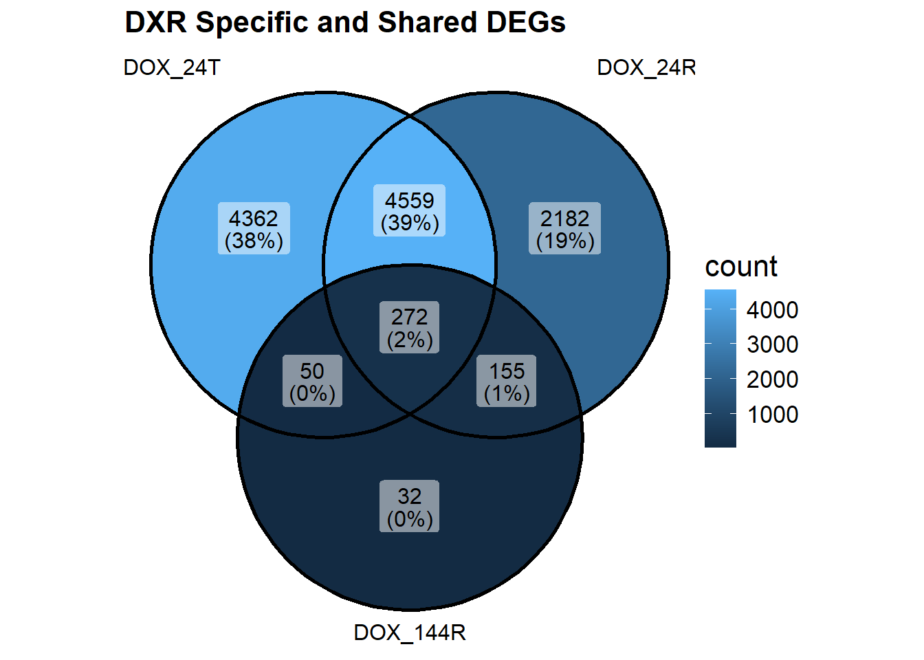
) + ggtitle("DXR Specific and Shared DEGs")+
theme(
plot.title = element_text(size = 16, face = "bold"), # Increase title size
text = element_text(size = 16) # Increase text size globally
)
| Version | Author | Date |
|---|---|---|
| 29a5c35 | emmapfort | 2025-05-16 |
#Now that I've made my venn diagram, I want to compare these DEGs
#set 1 : 4362 DOX24T specific genes
#set2 : 4362 + 4550 + 50 + 272 genes shared across DOX24T (all genes)
#how many of these are downregulated and how many are upregulated?
## Fit limma model using code as it is found in the original cormotif code. It has
## only been modified to add names to the matrix of t values, as well as the
## limma fits
limmafit.default <- function(exprs,groupid,compid) {
limmafits <- list()
compnum <- nrow(compid)
genenum <- nrow(exprs)
limmat <- matrix(0,genenum,compnum)
limmas2 <- rep(0,compnum)
limmadf <- rep(0,compnum)
limmav0 <- rep(0,compnum)
limmag1num <- rep(0,compnum)
limmag2num <- rep(0,compnum)
rownames(limmat) <- rownames(exprs)
colnames(limmat) <- rownames(compid)
names(limmas2) <- rownames(compid)
names(limmadf) <- rownames(compid)
names(limmav0) <- rownames(compid)
names(limmag1num) <- rownames(compid)
names(limmag2num) <- rownames(compid)
for(i in 1:compnum) {
selid1 <- which(groupid == compid[i,1])
selid2 <- which(groupid == compid[i,2])
eset <- new("ExpressionSet", exprs=cbind(exprs[,selid1],exprs[,selid2]))
g1num <- length(selid1)
g2num <- length(selid2)
designmat <- cbind(base=rep(1,(g1num+g2num)), delta=c(rep(0,g1num),rep(1,g2num)))
fit <- lmFit(eset,designmat)
fit <- eBayes(fit)
limmat[,i] <- fit$t[,2]
limmas2[i] <- fit$s2.prior
limmadf[i] <- fit$df.prior
limmav0[i] <- fit$var.prior[2]
limmag1num[i] <- g1num
limmag2num[i] <- g2num
limmafits[[i]] <- fit
# log odds
# w<-sqrt(1+fit$var.prior[2]/(1/g1num+1/g2num))
# log(0.99)+dt(fit$t[1,2],g1num+g2num-2+fit$df.prior,log=TRUE)-log(0.01)-dt(fit$t[1,2]/w, g1num+g2num-2+fit$df.prior, log=TRUE)+log(w)
}
names(limmafits) <- rownames(compid)
limmacompnum<-nrow(compid)
result<-list(t = limmat,
v0 = limmav0,
df0 = limmadf,
s20 = limmas2,
g1num = limmag1num,
g2num = limmag2num,
compnum = limmacompnum,
fits = limmafits)
}
limmafit.counts <-
function (exprs, groupid, compid, norm.factor.method = "TMM", voom.normalize.method = "none")
{
limmafits <- list()
compnum <- nrow(compid)
genenum <- nrow(exprs)
limmat <- matrix(NA,genenum,compnum)
limmas2 <- rep(0,compnum)
limmadf <- rep(0,compnum)
limmav0 <- rep(0,compnum)
limmag1num <- rep(0,compnum)
limmag2num <- rep(0,compnum)
rownames(limmat) <- rownames(exprs)
colnames(limmat) <- rownames(compid)
names(limmas2) <- rownames(compid)
names(limmadf) <- rownames(compid)
names(limmav0) <- rownames(compid)
names(limmag1num) <- rownames(compid)
names(limmag2num) <- rownames(compid)
for (i in 1:compnum) {
message(paste("Running limma for comparision",i,"/",compnum))
selid1 <- which(groupid == compid[i, 1])
selid2 <- which(groupid == compid[i, 2])
# make a new count data frame
counts <- cbind(exprs[, selid1], exprs[, selid2])
# remove NAs
not.nas <- which(apply(counts, 1, function(x) !any(is.na(x))) == TRUE)
# runn voom/limma
d <- DGEList(counts[not.nas,])
d <- calcNormFactors(d, method = norm.factor.method)
g1num <- length(selid1)
g2num <- length(selid2)
designmat <- cbind(base = rep(1, (g1num + g2num)), delta = c(rep(0,
g1num), rep(1, g2num)))
y <- voom(d, designmat, normalize.method = voom.normalize.method)
fit <- lmFit(y, designmat)
fit <- eBayes(fit)
limmafits[[i]] <- fit
limmat[not.nas, i] <- fit$t[, 2]
limmas2[i] <- fit$s2.prior
limmadf[i] <- fit$df.prior
limmav0[i] <- fit$var.prior[2]
limmag1num[i] <- g1num
limmag2num[i] <- g2num
}
limmacompnum <- nrow(compid)
names(limmafits) <- rownames(compid)
result <- list(t = limmat,
v0 = limmav0,
df0 = limmadf,
s20 = limmas2,
g1num = limmag1num,
g2num = limmag2num,
compnum = limmacompnum,
fits = limmafits)
}
limmafit.list <-
function (fitlist, cmp.idx=2)
{
compnum <- length(fitlist)
genes <- c()
for (i in 1:compnum) genes <- unique(c(genes, rownames(fitlist[[i]])))
genenum <- length(genes)
limmat <- matrix(NA,genenum,compnum)
limmas2 <- rep(0,compnum)
limmadf <- rep(0,compnum)
limmav0 <- rep(0,compnum)
limmag1num <- rep(0,compnum)
limmag2num <- rep(0,compnum)
rownames(limmat) <- genes
colnames(limmat) <- names(fitlist)
names(limmas2) <- names(fitlist)
names(limmadf) <- names(fitlist)
names(limmav0) <- names(fitlist)
names(limmag1num) <- names(fitlist)
names(limmag2num) <- names(fitlist)
for (i in 1:compnum) {
this.t <- fitlist[[i]]$t[,cmp.idx]
limmat[names(this.t),i] <- this.t
limmas2[i] <- fitlist[[i]]$s2.prior
limmadf[i] <- fitlist[[i]]$df.prior
limmav0[i] <- fitlist[[i]]$var.prior[cmp.idx]
limmag1num[i] <- sum(fitlist[[i]]$design[,cmp.idx]==0)
limmag2num[i] <- sum(fitlist[[i]]$design[,cmp.idx]==1)
}
limmacompnum <- compnum
result <- list(t = limmat,
v0 = limmav0,
df0 = limmadf,
s20 = limmas2,
g1num = limmag1num,
g2num = limmag2num,
compnum = limmacompnum,
fits = limmafits)
}
## Rank genes based on statistics
generank<-function(x) {
xcol<-ncol(x)
xrow<-nrow(x)
result<-matrix(0,xrow,xcol)
z<-(1:1:xrow)
for(i in 1:xcol) {
y<-sort(x[,i],decreasing=TRUE,na.last=TRUE)
result[,i]<-match(x[,i],y)
result[,i]<-order(result[,i])
}
result
}
## Log-likelihood for moderated t under H0
modt.f0.loglike<-function(x,df) {
a<-dt(x, df, log=TRUE)
result<-as.vector(a)
flag<-which(is.na(result)==TRUE)
result[flag]<-0
result
}
## Log-likelihood for moderated t under H1
## param=c(df,g1num,g2num,v0)
modt.f1.loglike<-function(x,param) {
df<-param[1]
g1num<-param[2]
g2num<-param[3]
v0<-param[4]
w<-sqrt(1+v0/(1/g1num+1/g2num))
dt(x/w, df, log=TRUE)-log(w)
a<-dt(x/w, df, log=TRUE)-log(w)
result<-as.vector(a)
flag<-which(is.na(result)==TRUE)
result[flag]<-0
result
}
## Correlation Motif Fit
cmfit.X<-function(x, type, K=1, tol=1e-3, max.iter=100) {
## initialize
xrow <- nrow(x)
xcol <- ncol(x)
loglike0 <- list()
loglike1 <- list()
p <- rep(1, K)/K
q <- matrix(runif(K * xcol), K, xcol)
q[1, ] <- rep(0.01, xcol)
for (i in 1:xcol) {
f0 <- type[[i]][[1]]
f0param <- type[[i]][[2]]
f1 <- type[[i]][[3]]
f1param <- type[[i]][[4]]
loglike0[[i]] <- f0(x[, i], f0param)
loglike1[[i]] <- f1(x[, i], f1param)
}
condlike <- list()
for (i in 1:xcol) {
condlike[[i]] <- matrix(0, xrow, K)
}
loglike.old <- -1e+10
for (i.iter in 1:max.iter) {
if ((i.iter%%50) == 0) {
print(paste("We have run the first ", i.iter, " iterations for K=",
K, sep = ""))
}
err <- tol + 1
clustlike <- matrix(0, xrow, K)
#templike <- matrix(0, xrow, 2)
templike1 <- rep(0, xrow)
templike2 <- rep(0, xrow)
for (j in 1:K) {
for (i in 1:xcol) {
templike1 <- log(q[j, i]) + loglike1[[i]]
templike2 <- log(1 - q[j, i]) + loglike0[[i]]
tempmax <- Rfast::Pmax(templike1, templike2)
templike1 <- exp(templike1 - tempmax)
templike2 <- exp(templike2 - tempmax)
tempsum <- templike1 + templike2
clustlike[, j] <- clustlike[, j] + tempmax +
log(tempsum)
condlike[[i]][, j] <- templike1/tempsum
}
clustlike[, j] <- clustlike[, j] + log(p[j])
}
#tempmax <- apply(clustlike, 1, max)
tempmax <- Rfast::rowMaxs(clustlike, value=TRUE)
for (j in 1:K) {
clustlike[, j] <- exp(clustlike[, j] - tempmax)
}
#tempsum <- apply(clustlike, 1, sum)
tempsum <- Rfast::rowsums(clustlike)
for (j in 1:K) {
clustlike[, j] <- clustlike[, j]/tempsum
}
#p.new <- (apply(clustlike, 2, sum) + 1)/(xrow + K)
p.new <- (Rfast::colsums(clustlike) + 1)/(xrow + K)
q.new <- matrix(0, K, xcol)
for (j in 1:K) {
clustpsum <- sum(clustlike[, j])
for (i in 1:xcol) {
q.new[j, i] <- (sum(clustlike[, j] * condlike[[i]][,
j]) + 1)/(clustpsum + 2)
}
}
err.p <- max(abs(p.new - p)/p)
err.q <- max(abs(q.new - q)/q)
err <- max(err.p, err.q)
loglike.new <- (sum(tempmax + log(tempsum)) + sum(log(p.new)) +
sum(log(q.new) + log(1 - q.new)))/xrow
p <- p.new
q <- q.new
loglike.old <- loglike.new
if (err < tol) {
break
}
}
clustlike <- matrix(0, xrow, K)
for (j in 1:K) {
for (i in 1:xcol) {
templike1 <- log(q[j, i]) + loglike1[[i]]
templike2 <- log(1 - q[j, i]) + loglike0[[i]]
tempmax <- Rfast::Pmax(templike1, templike2)
templike1 <- exp(templike1 - tempmax)
templike2 <- exp(templike2 - tempmax)
tempsum <- templike1 + templike2
clustlike[, j] <- clustlike[, j] + tempmax + log(tempsum)
condlike[[i]][, j] <- templike1/tempsum
}
clustlike[, j] <- clustlike[, j] + log(p[j])
}
#tempmax <- apply(clustlike, 1, max)
tempmax <- Rfast::rowMaxs(clustlike, value=TRUE)
for (j in 1:K) {
clustlike[, j] <- exp(clustlike[, j] - tempmax)
}
#tempsum <- apply(clustlike, 1, sum)
tempsum <- Rfast::rowsums(clustlike)
for (j in 1:K) {
clustlike[, j] <- clustlike[, j]/tempsum
}
p.post <- matrix(0, xrow, xcol)
for (j in 1:K) {
for (i in 1:xcol) {
p.post[, i] <- p.post[, i] + clustlike[, j] * condlike[[i]][,
j]
}
}
loglike.old <- loglike.old - (sum(log(p)) + sum(log(q) +
log(1 - q)))/xrow
loglike.old <- loglike.old * xrow
result <- list(p.post = p.post, motif.prior = p, motif.q = q,
loglike = loglike.old, clustlike=clustlike, condlike=condlike)
}
## Fit using (0,0,...,0) and (1,1,...,1)
cmfitall<-function(x, type, tol=1e-3, max.iter=100) {
## initialize
xrow<-nrow(x)
xcol<-ncol(x)
loglike0<-list()
loglike1<-list()
p<-0.01
## compute loglikelihood
L0<-matrix(0,xrow,1)
L1<-matrix(0,xrow,1)
for(i in 1:xcol) {
f0<-type[[i]][[1]]
f0param<-type[[i]][[2]]
f1<-type[[i]][[3]]
f1param<-type[[i]][[4]]
loglike0[[i]]<-f0(x[,i],f0param)
loglike1[[i]]<-f1(x[,i],f1param)
L0<-L0+loglike0[[i]]
L1<-L1+loglike1[[i]]
}
## EM algorithm to get MLE of p and q
loglike.old <- -1e10
for(i.iter in 1:max.iter) {
if((i.iter%%50) == 0) {
print(paste("We have run the first ", i.iter, " iterations",sep=""))
}
err<-tol+1
## compute posterior cluster membership
clustlike<-matrix(0,xrow,2)
clustlike[,1]<-log(1-p)+L0
clustlike[,2]<-log(p)+L1
tempmax<-apply(clustlike,1,max)
for(j in 1:2) {
clustlike[,j]<-exp(clustlike[,j]-tempmax)
}
tempsum<-apply(clustlike,1,sum)
## update motif occurrence rate
for(j in 1:2) {
clustlike[,j]<-clustlike[,j]/tempsum
}
p.new<-(sum(clustlike[,2])+1)/(xrow+2)
## evaluate convergence
err<-abs(p.new-p)/p
## evaluate whether the log.likelihood increases
loglike.new<-(sum(tempmax+log(tempsum))+log(p.new)+log(1-p.new))/xrow
loglike.old<-loglike.new
p<-p.new
if(err<tol) {
break;
}
}
## compute posterior p
clustlike<-matrix(0,xrow,2)
clustlike[,1]<-log(1-p)+L0
clustlike[,2]<-log(p)+L1
tempmax<-apply(clustlike,1,max)
for(j in 1:2) {
clustlike[,j]<-exp(clustlike[,j]-tempmax)
}
tempsum<-apply(clustlike,1,sum)
for(j in 1:2) {
clustlike[,j]<-clustlike[,j]/tempsum
}
p.post<-matrix(0,xrow,xcol)
for(i in 1:xcol) {
p.post[,i]<-clustlike[,2]
}
## return
#calculate back loglikelihood
loglike.old<-loglike.old-(log(p)+log(1-p))/xrow
loglike.old<-loglike.old*xrow
result<-list(p.post=p.post, motif.prior=p, loglike=loglike.old)
}
## Fit each dataset separately
cmfitsep<-function(x, type, tol=1e-3, max.iter=100) {
## initialize
xrow<-nrow(x)
xcol<-ncol(x)
loglike0<-list()
loglike1<-list()
p<-0.01*rep(1,xcol)
loglike.final<-rep(0,xcol)
## compute loglikelihood
for(i in 1:xcol) {
f0<-type[[i]][[1]]
f0param<-type[[i]][[2]]
f1<-type[[i]][[3]]
f1param<-type[[i]][[4]]
loglike0[[i]]<-f0(x[,i],f0param)
loglike1[[i]]<-f1(x[,i],f1param)
}
p.post<-matrix(0,xrow,xcol)
## EM algorithm to get MLE of p
for(coli in 1:xcol) {
loglike.old <- -1e10
for(i.iter in 1:max.iter) {
if((i.iter%%50) == 0) {
print(paste("We have run the first ", i.iter, " iterations",sep=""))
}
err<-tol+1
## compute posterior cluster membership
clustlike<-matrix(0,xrow,2)
clustlike[,1]<-log(1-p[coli])+loglike0[[coli]]
clustlike[,2]<-log(p[coli])+loglike1[[coli]]
tempmax<-apply(clustlike,1,max)
for(j in 1:2) {
clustlike[,j]<-exp(clustlike[,j]-tempmax)
}
tempsum<-apply(clustlike,1,sum)
## evaluate whether the log.likelihood increases
loglike.new<-sum(tempmax+log(tempsum))/xrow
## update motif occurrence rate
for(j in 1:2) {
clustlike[,j]<-clustlike[,j]/tempsum
}
p.new<-(sum(clustlike[,2]))/(xrow)
## evaluate convergence
err<-abs(p.new-p[coli])/p[coli]
loglike.old<-loglike.new
p[coli]<-p.new
if(err<tol) {
break;
}
}
## compute posterior p
clustlike<-matrix(0,xrow,2)
clustlike[,1]<-log(1-p[coli])+loglike0[[coli]]
clustlike[,2]<-log(p[coli])+loglike1[[coli]]
tempmax<-apply(clustlike,1,max)
for(j in 1:2) {
clustlike[,j]<-exp(clustlike[,j]-tempmax)
}
tempsum<-apply(clustlike,1,sum)
for(j in 1:2) {
clustlike[,j]<-clustlike[,j]/tempsum
}
p.post[,coli]<-clustlike[,2]
loglike.final[coli]<-loglike.old
}
## return
loglike.final<-loglike.final*xrow
result<-list(p.post=p.post, motif.prior=p, loglike=loglike.final)
}
## Fit the full model
cmfitfull<-function(x, type, tol=1e-3, max.iter=100) {
## initialize
xrow<-nrow(x)
xcol<-ncol(x)
loglike0<-list()
loglike1<-list()
K<-2^xcol
p<-rep(1,K)/K
pattern<-rep(0,xcol)
patid<-matrix(0,K,xcol)
## compute loglikelihood
for(i in 1:xcol) {
f0<-type[[i]][[1]]
f0param<-type[[i]][[2]]
f1<-type[[i]][[3]]
f1param<-type[[i]][[4]]
loglike0[[i]]<-f0(x[,i],f0param)
loglike1[[i]]<-f1(x[,i],f1param)
}
L<-matrix(0,xrow,K)
for(i in 1:K)
{
patid[i,]<-pattern
for(j in 1:xcol) {
if(pattern[j] < 0.5) {
L[,i]<-L[,i]+loglike0[[j]]
} else {
L[,i]<-L[,i]+loglike1[[j]]
}
}
if(i < K) {
pattern[xcol]<-pattern[xcol]+1
j<-xcol
while(pattern[j] > 1) {
pattern[j]<-0
j<-j-1
pattern[j]<-pattern[j]+1
}
}
}
## EM algorithm to get MLE of p and q
loglike.old <- -1e10
for(i.iter in 1:max.iter) {
if((i.iter%%50) == 0) {
print(paste("We have run the first ", i.iter, " iterations",sep=""))
}
err<-tol+1
## compute posterior cluster membership
clustlike<-matrix(0,xrow,K)
for(j in 1:K) {
clustlike[,j]<-log(p[j])+L[,j]
}
tempmax<-apply(clustlike,1,max)
for(j in 1:K) {
clustlike[,j]<-exp(clustlike[,j]-tempmax)
}
tempsum<-apply(clustlike,1,sum)
## update motif occurrence rate
for(j in 1:K) {
clustlike[,j]<-clustlike[,j]/tempsum
}
p.new<-(apply(clustlike,2,sum)+1)/(xrow+K)
## evaluate convergence
err<-max(abs(p.new-p)/p)
## evaluate whether the log.likelihood increases
loglike.new<-(sum(tempmax+log(tempsum))+sum(log(p.new)))/xrow
loglike.old<-loglike.new
p<-p.new
if(err<tol) {
break;
}
}
## compute posterior p
clustlike<-matrix(0,xrow,K)
for(j in 1:K) {
clustlike[,j]<-log(p[j])+L[,j]
}
tempmax<-apply(clustlike,1,max)
for(j in 1:K) {
clustlike[,j]<-exp(clustlike[,j]-tempmax)
}
tempsum<-apply(clustlike,1,sum)
for(j in 1:K) {
clustlike[,j]<-clustlike[,j]/tempsum
}
p.post<-matrix(0,xrow,xcol)
for(j in 1:K) {
for(i in 1:xcol) {
if(patid[j,i] > 0.5) {
p.post[,i]<-p.post[,i]+clustlike[,j]
}
}
}
## return
#calculate back loglikelihood
loglike.old<-loglike.old-sum(log(p))/xrow
loglike.old<-loglike.old*xrow
result<-list(p.post=p.post, motif.prior=p, loglike=loglike.old)
}
generatetype<-function(limfitted)
{
jtype<-list()
df<-limfitted$g1num+limfitted$g2num-2+limfitted$df0
for(j in 1:limfitted$compnum)
{
jtype[[j]]<-list(f0=modt.f0.loglike, f0.param=df[j], f1=modt.f1.loglike, f1.param=c(df[j],limfitted$g1num[j],limfitted$g2num[j],limfitted$v0[j]))
}
jtype
}
cormotiffit <- function(exprs, groupid=NULL, compid=NULL, K=1, tol=1e-3,
max.iter=100, BIC=TRUE, norm.factor.method="TMM",
voom.normalize.method = "none", runtype=c("logCPM","counts","limmafits"), each=3)
{
# first I want to do some typechecking. Input can be either a normalized
# matrix, a count matrix, or a list of limma fits. Dispatch the correct
# limmafit accordingly.
# todo: add some typechecking here
limfitted <- list()
if (runtype=="counts") {
limfitted <- limmafit.counts(exprs,groupid,compid, norm.factor.method, voom.normalize.method)
} else if (runtype=="logCPM") {
limfitted <- limmafit.default(exprs,groupid,compid)
} else if (runtype=="limmafits") {
limfitted <- limmafit.list(exprs)
} else {
stop("runtype must be one of 'logCPM', 'counts', or 'limmafits'")
}
jtype<-generatetype(limfitted)
fitresult<-list()
ks <- rep(K, each = each)
fitresult <- bplapply(1:length(ks), function(i, x, type, ks, tol, max.iter) {
cmfit.X(x, type, K = ks[i], tol = tol, max.iter = max.iter)
}, x=limfitted$t, type=jtype, ks=ks, tol=tol, max.iter=max.iter)
best.fitresults <- list()
for (i in 1:length(K)) {
w.k <- which(ks==K[i])
this.bic <- c()
for (j in w.k) this.bic[j] <- -2 * fitresult[[j]]$loglike + (K[i] - 1 + K[i] * limfitted$compnum) * log(dim(limfitted$t)[1])
w.min <- which(this.bic == min(this.bic, na.rm = TRUE))[1]
best.fitresults[[i]] <- fitresult[[w.min]]
}
fitresult <- best.fitresults
bic <- rep(0, length(K))
aic <- rep(0, length(K))
loglike <- rep(0, length(K))
for (i in 1:length(K)) loglike[i] <- fitresult[[i]]$loglike
for (i in 1:length(K)) bic[i] <- -2 * fitresult[[i]]$loglike + (K[i] - 1 + K[i] * limfitted$compnum) * log(dim(limfitted$t)[1])
for (i in 1:length(K)) aic[i] <- -2 * fitresult[[i]]$loglike + 2 * (K[i] - 1 + K[i] * limfitted$compnum)
if(BIC==TRUE) {
bestflag=which(bic==min(bic))
}
else {
bestflag=which(aic==min(aic))
}
result<-list(bestmotif=fitresult[[bestflag]],bic=cbind(K,bic),
aic=cbind(K,aic),loglike=cbind(K,loglike), allmotifs=fitresult)
}
cormotiffitall<-function(exprs,groupid,compid, tol=1e-3, max.iter=100)
{
limfitted<-limmafit(exprs,groupid,compid)
jtype<-generatetype(limfitted)
fitresult<-cmfitall(limfitted$t,type=jtype,tol=1e-3,max.iter=max.iter)
}
cormotiffitsep<-function(exprs,groupid,compid, tol=1e-3, max.iter=100)
{
limfitted<-limmafit(exprs,groupid,compid)
jtype<-generatetype(limfitted)
fitresult<-cmfitsep(limfitted$t,type=jtype,tol=1e-3,max.iter=max.iter)
}
cormotiffitfull<-function(exprs,groupid,compid, tol=1e-3, max.iter=100)
{
limfitted<-limmafit(exprs,groupid,compid)
jtype<-generatetype(limfitted)
fitresult<-cmfitfull(limfitted$t,type=jtype,tol=1e-3,max.iter=max.iter)
}
plotIC<-function(fitted_cormotif)
{
oldpar<-par(mfrow=c(1,2))
plot(fitted_cormotif$bic[,1], fitted_cormotif$bic[,2], type="b",xlab="Motif Number", ylab="BIC", main="BIC")
plot(fitted_cormotif$aic[,1], fitted_cormotif$aic[,2], type="b",xlab="Motif Number", ylab="AIC", main="AIC")
}
plotMotif<-function(fitted_cormotif,title="")
{
layout(matrix(1:2,ncol=2))
u<-1:dim(fitted_cormotif$bestmotif$motif.q)[2]
v<-1:dim(fitted_cormotif$bestmotif$motif.q)[1]
image(u,v,t(fitted_cormotif$bestmotif$motif.q),
col=gray(seq(from=1,to=0,by=-0.1)),xlab="Study",yaxt = "n",
ylab="Corr. Motifs",main=paste(title,"pattern",sep=" "))
axis(2,at=1:length(v))
for(i in 1:(length(u)+1))
{
abline(v=(i-0.5))
}
for(i in 1:(length(v)+1))
{
abline(h=(i-0.5))
}
Ng=10000
if(is.null(fitted_cormotif$bestmotif$p.post)!=TRUE)
Ng=nrow(fitted_cormotif$bestmotif$p.post)
genecount=floor(fitted_cormotif$bestmotif$motif.p*Ng)
NK=nrow(fitted_cormotif$bestmotif$motif.q)
plot(0,0.7,pch=".",xlim=c(0,1.2),ylim=c(0.75,NK+0.25),
frame.plot=FALSE,axes=FALSE,xlab="No. of genes",ylab="", main=paste(title,"frequency",sep=" "))
segments(0,0.7,fitted_cormotif$bestmotif$motif.p[1],0.7)
rect(0,1:NK-0.3,fitted_cormotif$bestmotif$motif.p,1:NK+0.3,
col="dark grey")
mtext(1:NK,at=1:NK,side=2,cex=0.8)
text(fitted_cormotif$bestmotif$motif.p+0.15,1:NK,
labels=floor(fitted_cormotif$bestmotif$motif.p*Ng))
}#Don't load me in if you're using the above function, as it has been modified above
library(Cormotif)Loading required package: affy
Attaching package: 'affy'The following object is masked from 'package:lubridate':
pm
Attaching package: 'Cormotif'The following objects are masked _by_ '.GlobalEnv':
cormotiffit, cormotiffitall, cormotiffitfull, cormotiffitsep,
generank, plotIC, plotMotif#input the cormotif matrix you're going to use
##this should be tmm normalized log2cpm
#the matrix that I used previously for limma was TMM counts - cpm this
#dge was the name of the DGE list object
cormotif_test <- cpm(dge, log = TRUE)
colnames(cormotif_test) <- (Metadata_2$Final_sample_name)
cormotif_counts <- dge
cormotif_test_df <- cormotif_test %>%
as.data.frame() %>%
rownames_to_column(., var = "Entrez_ID")
#write.csv(cormotif_test, "data/new/Cormotif_test_matrix.csv")
#reorder my test matrix to match the new groupid I've made
#I want my columns to be in this order:
#DOX24T 1-6, DOX24R 1-6, DOX144R 1-6, DMSO24T 1-6, DMSO24R 1-6, DMSO144R 1-6
Cormotif <- read.csv("data/new/Cormotif_matrix_final.csv")
dim(Cormotif)[1] 14319 37#14319 genes across 37 cols (1 is Entrez_ID)
Cormotif_df <- data.frame(Cormotif)
rownames(Cormotif_df) <- Cormotif_df$Entrez_ID
exprs.cormotif <- as.matrix(Cormotif_df[,2:37])
dim(exprs.cormotif)[1] 14319 36####make a test one to see if the TMM is causing issues or not
# Cormotif_cpm_test <- read.csv("data/new/filcpm_forCormotif.csv")
# dim(Cormotif_cpm_test)
#
# Cormotif_cpm_test_df <- data.frame(Cormotif_cpm_test)
#
# rownames(Cormotif_cpm_test_df) <- Cormotif_cpm_test_df$Entrez_ID
# exprs.cormotif_cpm_test <- as.matrix(Cormotif_cpm_test_df[,2:37])
# dim(exprs.cormotif_cpm_test)
####don't use this one, the previous is correct
#see what happens if you remove ind3 which is driving the response down?
#put together my group id and comparison id to make the correct comparisons between experimental conditions
#groupid tells which experimental conditions are grouped together
#compid tells which experimental conditions should be compared against one another
##ie DOX24T vs DMSO24T matched control
groupid_csv <- read.csv("data/new/GroupID.csv")
#now I have to make this into a vector (named vector)
groupid <- c(
DOX_24T_1 = 1, DOX_24T_2 = 1, DOX_24T_3 = 1, DOX_24T_4 = 1, DOX_24T_5 = 1, DOX_24T_6 = 1,
DOX_24R_1 = 2, DOX_24R_2 = 2, DOX_24R_3 = 2, DOX_24R_4 = 2, DOX_24R_5 = 2, DOX_24R_6 = 2,
DOX_144R_1 = 3, DOX_144R_2 = 3, DOX_144R_3 = 3, DOX_144R_4 = 3, DOX_144R_5 = 3, DOX_144R_6 = 3,
DMSO_24T_1 = 4, DMSO_24T_2 = 4, DMSO_24T_3 = 4, DMSO_24T_4 = 4, DMSO_24T_5 = 4, DMSO_24T_6 = 4,
DMSO_24R_1 = 5, DMSO_24R_2 = 5, DMSO_24R_3 = 5, DMSO_24R_4 = 5, DMSO_24R_5 = 5, DMSO_24R_6 = 5,
DMSO_144R_1 = 6, DMSO_144R_2 = 6, DMSO_144R_3 = 6, DMSO_144R_4 = 6, DMSO_144R_5 = 6, DMSO_144R_6 = 6
)
groupid_1 <- groupid %>% as.vector()
compid <- data.frame(Cond1 = c(1, 3, 5), Cond2 = c(2, 4, 6))#fit Cormotif model
set.seed(19191)
#only set the seed ONCE
motif.fitted <- cormotiffit(
exprs = exprs.cormotif,
groupid = groupid,
compid = compid,
K = 1:8,
max.iter = 1000,
BIC = TRUE,
runtype = "logCPM"
)[1] "We have run the first 50 iterations for K=1"
[1] "We have run the first 100 iterations for K=1"
[1] "We have run the first 50 iterations for K=1"
[1] "We have run the first 100 iterations for K=1"
[1] "We have run the first 50 iterations for K=1"
[1] "We have run the first 100 iterations for K=1"
[1] "We have run the first 50 iterations for K=2"
[1] "We have run the first 100 iterations for K=2"
[1] "We have run the first 150 iterations for K=2"
[1] "We have run the first 200 iterations for K=2"
[1] "We have run the first 250 iterations for K=2"
[1] "We have run the first 300 iterations for K=2"
[1] "We have run the first 350 iterations for K=2"
[1] "We have run the first 400 iterations for K=2"
[1] "We have run the first 450 iterations for K=2"[1] "We have run the first 50 iterations for K=2"
[1] "We have run the first 100 iterations for K=2"
[1] "We have run the first 150 iterations for K=2"
[1] "We have run the first 200 iterations for K=2"
[1] "We have run the first 250 iterations for K=2"
[1] "We have run the first 300 iterations for K=2"
[1] "We have run the first 350 iterations for K=2"
[1] "We have run the first 50 iterations for K=2"
[1] "We have run the first 100 iterations for K=2"
[1] "We have run the first 150 iterations for K=2"
[1] "We have run the first 200 iterations for K=2"
[1] "We have run the first 50 iterations for K=3"
[1] "We have run the first 100 iterations for K=3"
[1] "We have run the first 150 iterations for K=3"
[1] "We have run the first 200 iterations for K=3"
[1] "We have run the first 250 iterations for K=3"
[1] "We have run the first 300 iterations for K=3"
[1] "We have run the first 350 iterations for K=3"
[1] "We have run the first 400 iterations for K=3"
[1] "We have run the first 450 iterations for K=3"
[1] "We have run the first 500 iterations for K=3"
[1] "We have run the first 550 iterations for K=3"
[1] "We have run the first 600 iterations for K=3"
[1] "We have run the first 650 iterations for K=3"
[1] "We have run the first 700 iterations for K=3"
[1] "We have run the first 50 iterations for K=3"
[1] "We have run the first 100 iterations for K=3"
[1] "We have run the first 150 iterations for K=3"
[1] "We have run the first 200 iterations for K=3"
[1] "We have run the first 250 iterations for K=3"
[1] "We have run the first 300 iterations for K=3"
[1] "We have run the first 350 iterations for K=3"
[1] "We have run the first 400 iterations for K=3"
[1] "We have run the first 450 iterations for K=3"
[1] "We have run the first 500 iterations for K=3"
[1] "We have run the first 550 iterations for K=3"
[1] "We have run the first 600 iterations for K=3"
[1] "We have run the first 650 iterations for K=3"[1] "We have run the first 50 iterations for K=3"
[1] "We have run the first 100 iterations for K=3"
[1] "We have run the first 150 iterations for K=3"
[1] "We have run the first 200 iterations for K=3"
[1] "We have run the first 250 iterations for K=3"
[1] "We have run the first 300 iterations for K=3"
[1] "We have run the first 350 iterations for K=3"
[1] "We have run the first 400 iterations for K=3"
[1] "We have run the first 50 iterations for K=4"
[1] "We have run the first 100 iterations for K=4"
[1] "We have run the first 150 iterations for K=4"
[1] "We have run the first 200 iterations for K=4"
[1] "We have run the first 50 iterations for K=4"
[1] "We have run the first 100 iterations for K=4"
[1] "We have run the first 150 iterations for K=4"
[1] "We have run the first 200 iterations for K=4"
[1] "We have run the first 250 iterations for K=4"
[1] "We have run the first 300 iterations for K=4"
[1] "We have run the first 350 iterations for K=4"
[1] "We have run the first 400 iterations for K=4"
[1] "We have run the first 450 iterations for K=4"
[1] "We have run the first 500 iterations for K=4"
[1] "We have run the first 550 iterations for K=4"
[1] "We have run the first 600 iterations for K=4"
[1] "We have run the first 650 iterations for K=4"
[1] "We have run the first 50 iterations for K=4"
[1] "We have run the first 100 iterations for K=4"
[1] "We have run the first 150 iterations for K=4"
[1] "We have run the first 200 iterations for K=4"[1] "We have run the first 50 iterations for K=5"
[1] "We have run the first 100 iterations for K=5"
[1] "We have run the first 150 iterations for K=5"
[1] "We have run the first 200 iterations for K=5"
[1] "We have run the first 250 iterations for K=5"
[1] "We have run the first 300 iterations for K=5"
[1] "We have run the first 350 iterations for K=5"
[1] "We have run the first 400 iterations for K=5"
[1] "We have run the first 450 iterations for K=5"
[1] "We have run the first 500 iterations for K=5"
[1] "We have run the first 550 iterations for K=5"
[1] "We have run the first 50 iterations for K=5"
[1] "We have run the first 100 iterations for K=5"
[1] "We have run the first 150 iterations for K=5"
[1] "We have run the first 200 iterations for K=5"
[1] "We have run the first 250 iterations for K=5"
[1] "We have run the first 300 iterations for K=5"
[1] "We have run the first 350 iterations for K=5"
[1] "We have run the first 400 iterations for K=5"
[1] "We have run the first 450 iterations for K=5"
[1] "We have run the first 500 iterations for K=5"
[1] "We have run the first 550 iterations for K=5"
[1] "We have run the first 600 iterations for K=5"
[1] "We have run the first 650 iterations for K=5"
[1] "We have run the first 700 iterations for K=5"
[1] "We have run the first 750 iterations for K=5"
[1] "We have run the first 800 iterations for K=5"
[1] "We have run the first 850 iterations for K=5"
[1] "We have run the first 900 iterations for K=5"
[1] "We have run the first 950 iterations for K=5"
[1] "We have run the first 1000 iterations for K=5"
[1] "We have run the first 50 iterations for K=5"
[1] "We have run the first 100 iterations for K=5"
[1] "We have run the first 150 iterations for K=5"
[1] "We have run the first 200 iterations for K=5"
[1] "We have run the first 250 iterations for K=5"
[1] "We have run the first 300 iterations for K=5"
[1] "We have run the first 350 iterations for K=5"
[1] "We have run the first 400 iterations for K=5"
[1] "We have run the first 450 iterations for K=5"
[1] "We have run the first 500 iterations for K=5"
[1] "We have run the first 550 iterations for K=5"
[1] "We have run the first 600 iterations for K=5"
[1] "We have run the first 650 iterations for K=5"
[1] "We have run the first 700 iterations for K=5"
[1] "We have run the first 750 iterations for K=5"
[1] "We have run the first 800 iterations for K=5"
[1] "We have run the first 50 iterations for K=6"
[1] "We have run the first 100 iterations for K=6"
[1] "We have run the first 150 iterations for K=6"
[1] "We have run the first 200 iterations for K=6"
[1] "We have run the first 250 iterations for K=6"
[1] "We have run the first 300 iterations for K=6"
[1] "We have run the first 350 iterations for K=6"
[1] "We have run the first 400 iterations for K=6"
[1] "We have run the first 450 iterations for K=6"
[1] "We have run the first 500 iterations for K=6"
[1] "We have run the first 550 iterations for K=6"
[1] "We have run the first 600 iterations for K=6"
[1] "We have run the first 650 iterations for K=6"
[1] "We have run the first 700 iterations for K=6"
[1] "We have run the first 750 iterations for K=6"
[1] "We have run the first 800 iterations for K=6"
[1] "We have run the first 850 iterations for K=6"
[1] "We have run the first 900 iterations for K=6"
[1] "We have run the first 950 iterations for K=6"
[1] "We have run the first 1000 iterations for K=6"[1] "We have run the first 50 iterations for K=6"
[1] "We have run the first 100 iterations for K=6"
[1] "We have run the first 150 iterations for K=6"
[1] "We have run the first 200 iterations for K=6"
[1] "We have run the first 250 iterations for K=6"
[1] "We have run the first 300 iterations for K=6"
[1] "We have run the first 350 iterations for K=6"
[1] "We have run the first 400 iterations for K=6"
[1] "We have run the first 450 iterations for K=6"
[1] "We have run the first 500 iterations for K=6"
[1] "We have run the first 550 iterations for K=6"
[1] "We have run the first 600 iterations for K=6"
[1] "We have run the first 650 iterations for K=6"
[1] "We have run the first 700 iterations for K=6"
[1] "We have run the first 750 iterations for K=6"
[1] "We have run the first 800 iterations for K=6"
[1] "We have run the first 850 iterations for K=6"
[1] "We have run the first 50 iterations for K=6"
[1] "We have run the first 100 iterations for K=6"
[1] "We have run the first 150 iterations for K=6"
[1] "We have run the first 200 iterations for K=6"
[1] "We have run the first 250 iterations for K=6"
[1] "We have run the first 300 iterations for K=6"
[1] "We have run the first 350 iterations for K=6"
[1] "We have run the first 400 iterations for K=6"
[1] "We have run the first 450 iterations for K=6"
[1] "We have run the first 500 iterations for K=6"
[1] "We have run the first 550 iterations for K=6"
[1] "We have run the first 600 iterations for K=6"
[1] "We have run the first 650 iterations for K=6"
[1] "We have run the first 700 iterations for K=6"
[1] "We have run the first 750 iterations for K=6"
[1] "We have run the first 800 iterations for K=6"
[1] "We have run the first 50 iterations for K=7"
[1] "We have run the first 100 iterations for K=7"
[1] "We have run the first 150 iterations for K=7"
[1] "We have run the first 200 iterations for K=7"
[1] "We have run the first 250 iterations for K=7"
[1] "We have run the first 300 iterations for K=7"
[1] "We have run the first 350 iterations for K=7"
[1] "We have run the first 400 iterations for K=7"
[1] "We have run the first 450 iterations for K=7"
[1] "We have run the first 500 iterations for K=7"
[1] "We have run the first 550 iterations for K=7"
[1] "We have run the first 600 iterations for K=7"
[1] "We have run the first 650 iterations for K=7"
[1] "We have run the first 700 iterations for K=7"
[1] "We have run the first 750 iterations for K=7"
[1] "We have run the first 800 iterations for K=7"
[1] "We have run the first 850 iterations for K=7"
[1] "We have run the first 900 iterations for K=7"
[1] "We have run the first 950 iterations for K=7"
[1] "We have run the first 1000 iterations for K=7"
[1] "We have run the first 50 iterations for K=7"
[1] "We have run the first 100 iterations for K=7"
[1] "We have run the first 150 iterations for K=7"
[1] "We have run the first 200 iterations for K=7"
[1] "We have run the first 250 iterations for K=7"
[1] "We have run the first 300 iterations for K=7"
[1] "We have run the first 350 iterations for K=7"
[1] "We have run the first 400 iterations for K=7"
[1] "We have run the first 450 iterations for K=7"
[1] "We have run the first 500 iterations for K=7"
[1] "We have run the first 550 iterations for K=7"
[1] "We have run the first 600 iterations for K=7"
[1] "We have run the first 650 iterations for K=7"
[1] "We have run the first 700 iterations for K=7"[1] "We have run the first 50 iterations for K=7"
[1] "We have run the first 100 iterations for K=7"
[1] "We have run the first 150 iterations for K=7"
[1] "We have run the first 200 iterations for K=7"
[1] "We have run the first 250 iterations for K=7"
[1] "We have run the first 300 iterations for K=7"
[1] "We have run the first 350 iterations for K=7"
[1] "We have run the first 400 iterations for K=7"
[1] "We have run the first 450 iterations for K=7"
[1] "We have run the first 500 iterations for K=7"
[1] "We have run the first 550 iterations for K=7"
[1] "We have run the first 600 iterations for K=7"
[1] "We have run the first 650 iterations for K=7"
[1] "We have run the first 700 iterations for K=7"
[1] "We have run the first 750 iterations for K=7"
[1] "We have run the first 800 iterations for K=7"
[1] "We have run the first 850 iterations for K=7"
[1] "We have run the first 900 iterations for K=7"
[1] "We have run the first 950 iterations for K=7"
[1] "We have run the first 1000 iterations for K=7"
[1] "We have run the first 50 iterations for K=8"
[1] "We have run the first 100 iterations for K=8"
[1] "We have run the first 150 iterations for K=8"
[1] "We have run the first 200 iterations for K=8"
[1] "We have run the first 250 iterations for K=8"
[1] "We have run the first 300 iterations for K=8"
[1] "We have run the first 350 iterations for K=8"
[1] "We have run the first 400 iterations for K=8"
[1] "We have run the first 450 iterations for K=8"
[1] "We have run the first 500 iterations for K=8"
[1] "We have run the first 550 iterations for K=8"
[1] "We have run the first 600 iterations for K=8"
[1] "We have run the first 650 iterations for K=8"
[1] "We have run the first 700 iterations for K=8"
[1] "We have run the first 750 iterations for K=8"
[1] "We have run the first 800 iterations for K=8"
[1] "We have run the first 850 iterations for K=8"
[1] "We have run the first 900 iterations for K=8"
[1] "We have run the first 950 iterations for K=8"
[1] "We have run the first 1000 iterations for K=8"
[1] "We have run the first 50 iterations for K=8"
[1] "We have run the first 100 iterations for K=8"
[1] "We have run the first 150 iterations for K=8"
[1] "We have run the first 200 iterations for K=8"
[1] "We have run the first 250 iterations for K=8"
[1] "We have run the first 300 iterations for K=8"
[1] "We have run the first 350 iterations for K=8"
[1] "We have run the first 400 iterations for K=8"
[1] "We have run the first 450 iterations for K=8"
[1] "We have run the first 500 iterations for K=8"
[1] "We have run the first 550 iterations for K=8"
[1] "We have run the first 600 iterations for K=8"
[1] "We have run the first 650 iterations for K=8"
[1] "We have run the first 700 iterations for K=8"
[1] "We have run the first 750 iterations for K=8"
[1] "We have run the first 800 iterations for K=8"
[1] "We have run the first 850 iterations for K=8"
[1] "We have run the first 900 iterations for K=8"
[1] "We have run the first 950 iterations for K=8"
[1] "We have run the first 1000 iterations for K=8"#plot BIC and AIC to see which number of motifs was best for both models
plotIC(motif.fitted)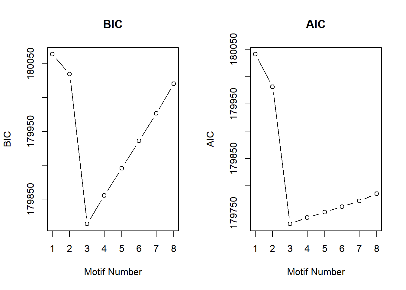
| Version | Author | Date |
|---|---|---|
| 29a5c35 | emmapfort | 2025-05-16 |
motif.fitted$bic K bic
[1,] 1 180063.9
[2,] 2 180034.4
[3,] 3 179813.4
[4,] 4 179855.6
[5,] 5 179895.7
[6,] 6 179936.2
[7,] 7 179976.6
[8,] 8 180020.3#now plot the motifs themselves
plotMotif(motif.fitted, title = "Fitted Motifs for DXR")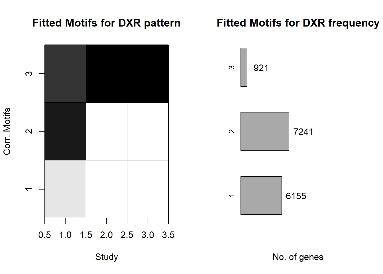
| Version | Author | Date |
|---|---|---|
| 29a5c35 | emmapfort | 2025-05-16 |
#extract the posterior probability that these DEGs belong to motifs
gene_prob_all <- motif.fitted$bestmotif$p.post
rownames(gene_prob_all) <- rownames(Cormotif_df)

#extract the cluster likelihood - which DEGs are most likely to be in this cluster
motif_prob <- motif.fitted$bestmotif$clustlike
rownames(motif_prob) <- rownames(gene_prob_all)
#write.csv(motif_prob,"data/new/cormotif_probability_genelist_all.csv")

# Define gene probability groups
prob_all_1  <- rownames(gene_prob_all[(gene_prob_all[,1] >= 0.25 & gene_prob_all[,2] <0.5 & gene_prob_all[,3] <0.5),])

length(prob_all_1)
[1] 8646prob_all_2 <- rownames(gene_prob_all[(gene_prob_all[,1] >=0.3 & gene_prob_all[,2] >0.5 & gene_prob_all[,3] >0.5),])
length(prob_all_2)[1] 552prob_all_3 <- rownames(gene_prob_all[(gene_prob_all[,1] >0.5 & gene_prob_all[,2] <0.5 & gene_prob_all[,3] <0.5),])
length(prob_all_3)[1] 6353
sessionInfo()R version 4.4.2 (2024-10-31 ucrt)
Platform: x86_64-w64-mingw32/x64
Running under: Windows 11 x64 (build 22000)
Matrix products: default
locale:
[1] LC_COLLATE=English_United States.utf8
[2] LC_CTYPE=English_United States.utf8
[3] LC_MONETARY=English_United States.utf8
[4] LC_NUMERIC=C
[5] LC_TIME=English_United States.utf8
time zone: America/Chicago
tzcode source: internal
attached base packages:
[1] grid stats4 stats graphics grDevices utils datasets
[8] methods base
other attached packages:
[1] Cormotif_1.52.0 affy_1.84.0 BiocParallel_1.40.0
[4] ggpubr_0.6.0 UpSetR_1.4.0 ggVennDiagram_1.5.2
[7] reshape2_1.4.4 circlize_0.4.16 ComplexHeatmap_2.22.0
[10] org.Hs.eg.db_3.20.0 AnnotationDbi_1.68.0 IRanges_2.40.0
[13] S4Vectors_0.44.0 corrplot_0.95 ggfortify_0.4.17
[16] ggrepel_0.9.6 biomaRt_2.62.1 scales_1.4.0
[19] edgebundleR_0.1.4 edgeR_4.4.0 limma_3.62.1
[22] Biobase_2.66.0 BiocGenerics_0.52.0 lubridate_1.9.4
[25] forcats_1.0.0 stringr_1.5.1 dplyr_1.1.4
[28] purrr_1.0.4 readr_2.1.5 tidyr_1.3.1
[31] tibble_3.2.1 ggplot2_3.5.2 tidyverse_2.0.0
[34] workflowr_1.7.1
loaded via a namespace (and not attached):
[1] RColorBrewer_1.1-3 rstudioapi_0.17.1 jsonlite_2.0.0
[4] shape_1.4.6.1 magrittr_2.0.3 farver_2.1.2
[7] rmarkdown_2.29 GlobalOptions_0.1.2 fs_1.6.6
[10] zlibbioc_1.52.0 vctrs_0.6.5 memoise_2.0.1
[13] rstatix_0.7.2 htmltools_0.5.8.1 progress_1.2.3
[16] curl_6.0.1 broom_1.0.8 Formula_1.2-5
[19] sass_0.4.10 bslib_0.9.0 htmlwidgets_1.6.4
[22] plyr_1.8.9 httr2_1.1.2 cachem_1.1.0
[25] whisker_0.4.1 igraph_2.1.4 mime_0.13
[28] lifecycle_1.0.4 iterators_1.0.14 pkgconfig_2.0.3
[31] R6_2.6.1 fastmap_1.2.0 GenomeInfoDbData_1.2.13
[34] shiny_1.10.0 clue_0.3-66 digest_0.6.37
[37] colorspace_2.1-1 ps_1.9.1 rprojroot_2.0.4
[40] RSQLite_2.3.9 labeling_0.4.3 filelock_1.0.3
[43] timechange_0.3.0 abind_1.4-8 httr_1.4.7
[46] compiler_4.4.2 bit64_4.5.2 withr_3.0.2
[49] doParallel_1.0.17 backports_1.5.0 carData_3.0-5
[52] DBI_1.2.3 ggsignif_0.6.4 rappdirs_0.3.3
[55] rjson_0.2.23 tools_4.4.2 httpuv_1.6.16
[58] glue_1.8.0 callr_3.7.6 promises_1.3.2
[61] getPass_0.2-4 cluster_2.1.6 snow_0.4-4
[64] generics_0.1.3 gtable_0.3.6 tzdb_0.5.0
[67] preprocessCore_1.68.0 hms_1.1.3 car_3.1-3
[70] xml2_1.3.8 XVector_0.46.0 foreach_1.5.2
[73] pillar_1.10.2 later_1.4.2 BiocFileCache_2.14.0
[76] lattice_0.22-6 bit_4.5.0 tidyselect_1.2.1
[79] locfit_1.5-9.12 Biostrings_2.74.0 knitr_1.50
[82] git2r_0.36.2 gridExtra_2.3 xfun_0.52
[85] statmod_1.5.0 matrixStats_1.5.0 stringi_1.8.7
[88] UCSC.utils_1.2.0 yaml_2.3.10 evaluate_1.0.3
[91] codetools_0.2-20 BiocManager_1.30.25 affyio_1.76.0
[94] cli_3.6.3 xtable_1.8-4 processx_3.8.6
[97] jquerylib_0.1.4 Rcpp_1.0.14 GenomeInfoDb_1.42.3
[100] dbplyr_2.5.0 png_0.1-8 parallel_4.4.2
[103] blob_1.2.4 prettyunits_1.2.0 crayon_1.5.3
[106] GetoptLong_1.0.5 rlang_1.1.6 KEGGREST_1.46.0