5FU Recovery RNAseq Analysis

workflowr

• Summary
• Checks
• Past versions

Last updated: 2025-02-27

Checks: 7 0

Knit directory: Recovery_5FU/

This reproducible R Markdown analysis was created with workflowr (version 1.7.1). The Checks tab describes the reproducibility checks that were applied when the results were created. The Past versions tab lists the development history.

---

R Markdown file: up-to-date

Great! Since the R Markdown file has been committed to the Git repository, you know the exact version of the code that produced these results.

Environment: empty

Great job! The global environment was empty. Objects defined in the global environment can affect the analysis in your R Markdown file in unknown ways. For reproduciblity it’s best to always run the code in an empty environment.

Seed: set.seed(20250217)

The command set.seed(20250217) was run prior to running the code in the R Markdown file. Setting a seed ensures that any results that rely on randomness, e.g. subsampling or permutations, are reproducible.

Session information: recorded

Great job! Recording the operating system, R version, and package versions is critical for reproducibility.

Cache: none

Nice! There were no cached chunks for this analysis, so you can be confident that you successfully produced the results during this run.

File paths: relative

Great job! Using relative paths to the files within your workflowr project makes it easier to run your code on other machines.

Repository version: b086ed1

Great! You are using Git for version control. Tracking code development and connecting the code version to the results is critical for reproducibility.

The results in this page were generated with repository version b086ed1. See the Past versions tab to see a history of the changes made to the R Markdown and HTML files.

Note that you need to be careful to ensure that all relevant files for the analysis have been committed to Git prior to generating the results (you can use wflow_publish or wflow_git_commit). workflowr only checks the R Markdown file, but you know if there are other scripts or data files that it depends on. Below is the status of the Git repository when the results were generated:

Ignored files:
    Ignored:    .Rhistory
    Ignored:    .Rproj.user/

Note that any generated files, e.g. HTML, png, CSS, etc., are not included in this status report because it is ok for generated content to have uncommitted changes.

---

These are the previous versions of the repository in which changes were made to the R Markdown (analysis/Recovery_DE.Rmd) and HTML (docs/Recovery_DE.html) files. If you’ve configured a remote Git repository (see ?wflow_git_remote), click on the hyperlinks in the table below to view the files as they were in that past version.

File	Version	Author	Date	Message
Rmd	b086ed1	emmapfort	2025-02-27	wflow_publish(files = "analysis/Recovery_DE.Rmd")
html	41aef30	emmapfort	2025-02-27	Build site.
Rmd	e77e0d4	emmapfort	2025-02-27	Make website cohesive and dataframes concise.

---

Welcome to my research website.

── Attaching core tidyverse packages ──────────────────────── tidyverse 2.0.0 ──
✔ dplyr     1.1.4     ✔ readr     2.1.5
✔ forcats   1.0.0     ✔ stringr   1.5.1
✔ lubridate 1.9.3     ✔ tidyr     1.3.1
✔ purrr     1.0.2     
── Conflicts ────────────────────────────────────────── tidyverse_conflicts() ──
✖ dplyr::filter() masks stats::filter()
✖ dplyr::lag()    masks stats::lag()
ℹ Use the conflicted package (<http://conflicted.r-lib.org/>) to force all conflicts to become errors
Loading required package: limma

Loading required package: ggrepel


Attaching package: 'PCAtools'


The following objects are masked from 'package:stats':

    biplot, screeplot


Loading required package: affy

Loading required package: BiocGenerics


Attaching package: 'BiocGenerics'


The following object is masked from 'package:limma':

    plotMA


The following objects are masked from 'package:lubridate':

    intersect, setdiff, union


The following objects are masked from 'package:dplyr':

    combine, intersect, setdiff, union


The following objects are masked from 'package:stats':

    IQR, mad, sd, var, xtabs


The following objects are masked from 'package:base':

    anyDuplicated, aperm, append, as.data.frame, basename, cbind,
    colnames, dirname, do.call, duplicated, eval, evalq, Filter, Find,
    get, grep, grepl, intersect, is.unsorted, lapply, Map, mapply,
    match, mget, order, paste, pmax, pmax.int, pmin, pmin.int,
    Position, rank, rbind, Reduce, rownames, sapply, saveRDS, setdiff,
    table, tapply, union, unique, unsplit, which.max, which.min


Loading required package: Biobase

Welcome to Bioconductor

    Vignettes contain introductory material; view with
    'browseVignettes()'. To cite Bioconductor, see
    'citation("Biobase")', and for packages 'citation("pkgname")'.



Attaching package: 'affy'


The following object is masked from 'package:lubridate':

    pm


Loading required package: EDASeq

Loading required package: ShortRead

Loading required package: BiocParallel

Loading required package: Biostrings

Loading required package: S4Vectors

Loading required package: stats4


Attaching package: 'S4Vectors'


The following objects are masked from 'package:lubridate':

    second, second<-


The following objects are masked from 'package:dplyr':

    first, rename


The following object is masked from 'package:tidyr':

    expand


The following object is masked from 'package:utils':

    findMatches


The following objects are masked from 'package:base':

    expand.grid, I, unname


Loading required package: IRanges


Attaching package: 'IRanges'


The following object is masked from 'package:lubridate':

    %within%


The following objects are masked from 'package:dplyr':

    collapse, desc, slice


The following object is masked from 'package:purrr':

    reduce


The following object is masked from 'package:grDevices':

    windows


Loading required package: XVector


Attaching package: 'XVector'


The following object is masked from 'package:purrr':

    compact


Loading required package: GenomeInfoDb


Attaching package: 'Biostrings'


The following object is masked from 'package:base':

    strsplit


Loading required package: Rsamtools

Loading required package: GenomicRanges

Loading required package: GenomicAlignments

Loading required package: SummarizedExperiment

Loading required package: MatrixGenerics

Loading required package: matrixStats


Attaching package: 'matrixStats'


The following objects are masked from 'package:Biobase':

    anyMissing, rowMedians


The following object is masked from 'package:dplyr':

    count



Attaching package: 'MatrixGenerics'


The following objects are masked from 'package:matrixStats':

    colAlls, colAnyNAs, colAnys, colAvgsPerRowSet, colCollapse,
    colCounts, colCummaxs, colCummins, colCumprods, colCumsums,
    colDiffs, colIQRDiffs, colIQRs, colLogSumExps, colMadDiffs,
    colMads, colMaxs, colMeans2, colMedians, colMins, colOrderStats,
    colProds, colQuantiles, colRanges, colRanks, colSdDiffs, colSds,
    colSums2, colTabulates, colVarDiffs, colVars, colWeightedMads,
    colWeightedMeans, colWeightedMedians, colWeightedSds,
    colWeightedVars, rowAlls, rowAnyNAs, rowAnys, rowAvgsPerColSet,
    rowCollapse, rowCounts, rowCummaxs, rowCummins, rowCumprods,
    rowCumsums, rowDiffs, rowIQRDiffs, rowIQRs, rowLogSumExps,
    rowMadDiffs, rowMads, rowMaxs, rowMeans2, rowMedians, rowMins,
    rowOrderStats, rowProds, rowQuantiles, rowRanges, rowRanks,
    rowSdDiffs, rowSds, rowSums2, rowTabulates, rowVarDiffs, rowVars,
    rowWeightedMads, rowWeightedMeans, rowWeightedMedians,
    rowWeightedSds, rowWeightedVars


The following object is masked from 'package:Biobase':

    rowMedians



Attaching package: 'GenomicAlignments'


The following object is masked from 'package:dplyr':

    last



Attaching package: 'ShortRead'


The following object is masked from 'package:affy':

    intensity


The following object is masked from 'package:dplyr':

    id


The following object is masked from 'package:purrr':

    compose


The following object is masked from 'package:tibble':

    view

These samples (63 in total) have been aligned to the Ensembl 113 release of GRCh38 via subread, and counts have been generated using featureCounts with inbuilt hg38 genome

Data is located under 5FU Project on my computer All analysis saved in RDirectory Recovery_RNAseq

Individual 1 - 84-1 (9 samples)

Individual 2 - 87-1 (9 samples)

Individual 3 - 75-1 (9 samples)

Individual 4 - 75-1 (9 samples)

Individual 5 - 17-3 (9 samples)

Individual 6 - 90-1 (9 samples)

Individual 7 - 90-1 REP (9 samples)

Now that I have imported all of these counts files, I will make a matrix with all of the samples

First I’ll break them up by individual, and then combine them all together

Now that I’ve made individual matrices for each individual - I will combine them together into one large matrix

Past versions of "Counts Matrix All Individuals-1.png"

Version	Author	Date
41aef30	emmapfort	2025-02-27

Past versions of "Counts Matrix All Individuals-2.png"

Version	Author	Date
41aef30	emmapfort	2025-02-27

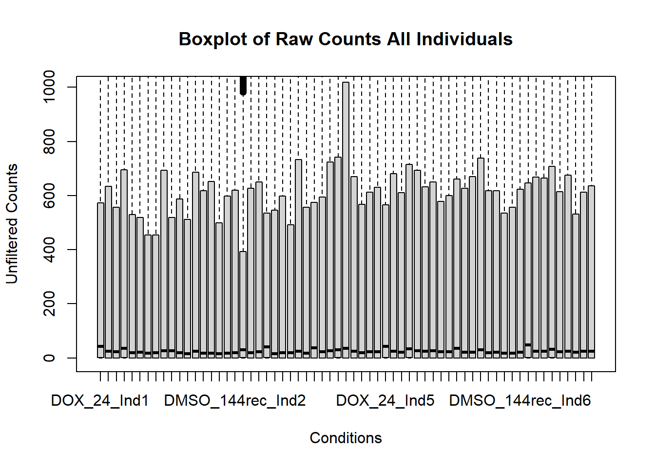
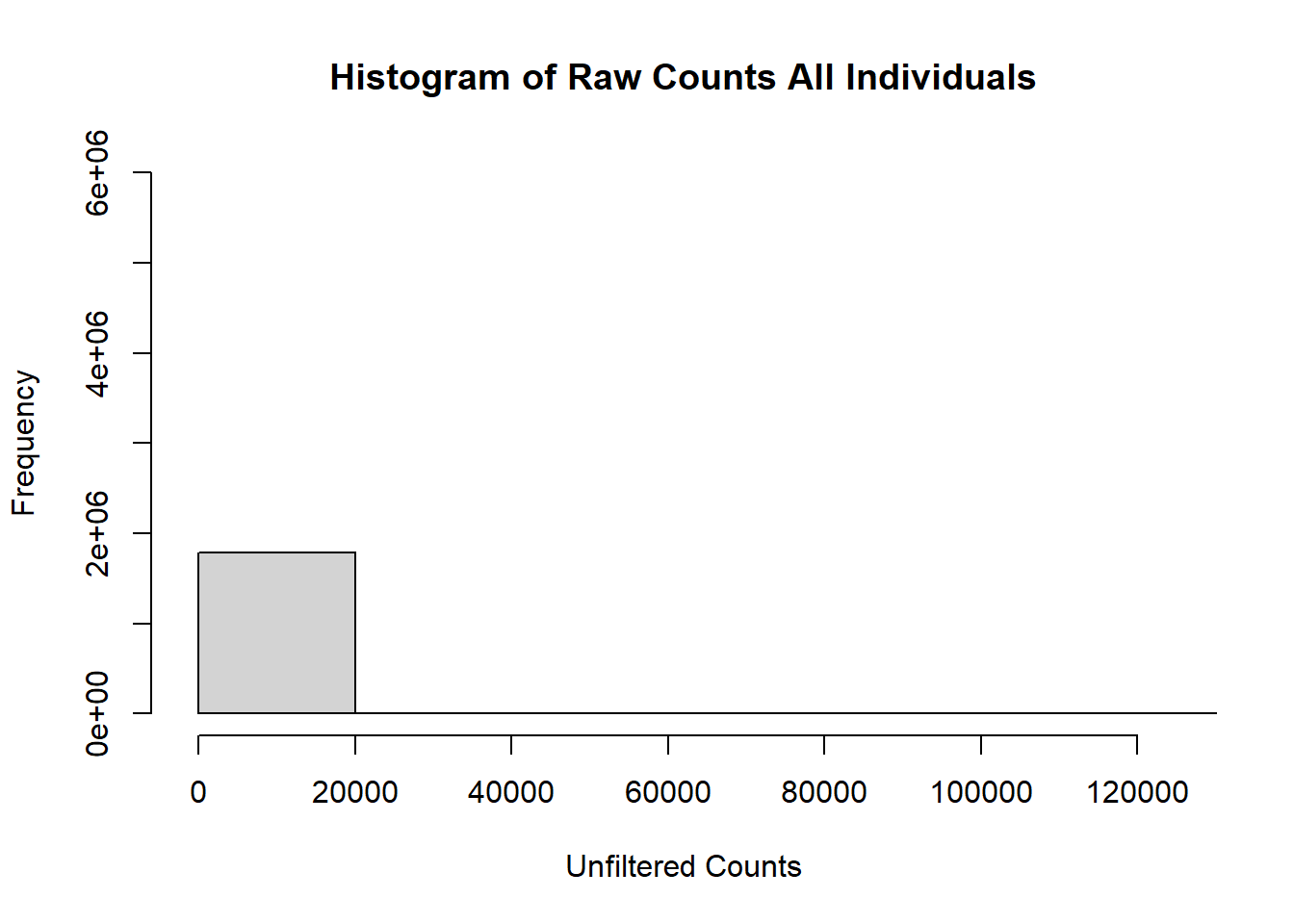
#Now that I've put together my matrix - I will do some QC checks

#now that I have all of my factors and my gene info, I will make some graphs to show the QC data

reads_by_sample <- c(tx_col)
fC_AllCounts %>% 
  ggplot(., aes (x = Conditions, y = Total_Align, fill = Treatment, group_by = Line))+
  geom_col()+
 geom_hline(aes(yintercept=20000000))+
 scale_fill_manual(values=reads_by_sample)+
  ggtitle(expression("Total number of reads by sample"))+
  xlab("")+
  ylab(expression("RNA-sequencing reads"))+
  theme_bw()+
  theme(plot.title = element_text(size = rel(2), hjust = 0.5),
        axis.title = element_text(size = 15, color = "black"),
        axis.ticks = element_line(linewidth = 1.5),
        axis.line = element_line(linewidth = 1.5),
        axis.text.y = element_text(size =10, color = "black", angle = 0, hjust = 0.8, vjust = 0.5),
        axis.text.x = element_text(size =10, color = "black", angle = 90, hjust = 1, vjust = 0.2),
        #strip.text.x = element_text(size = 15, color = "black", face = "bold"),
        strip.text.y = element_text(color = "white"))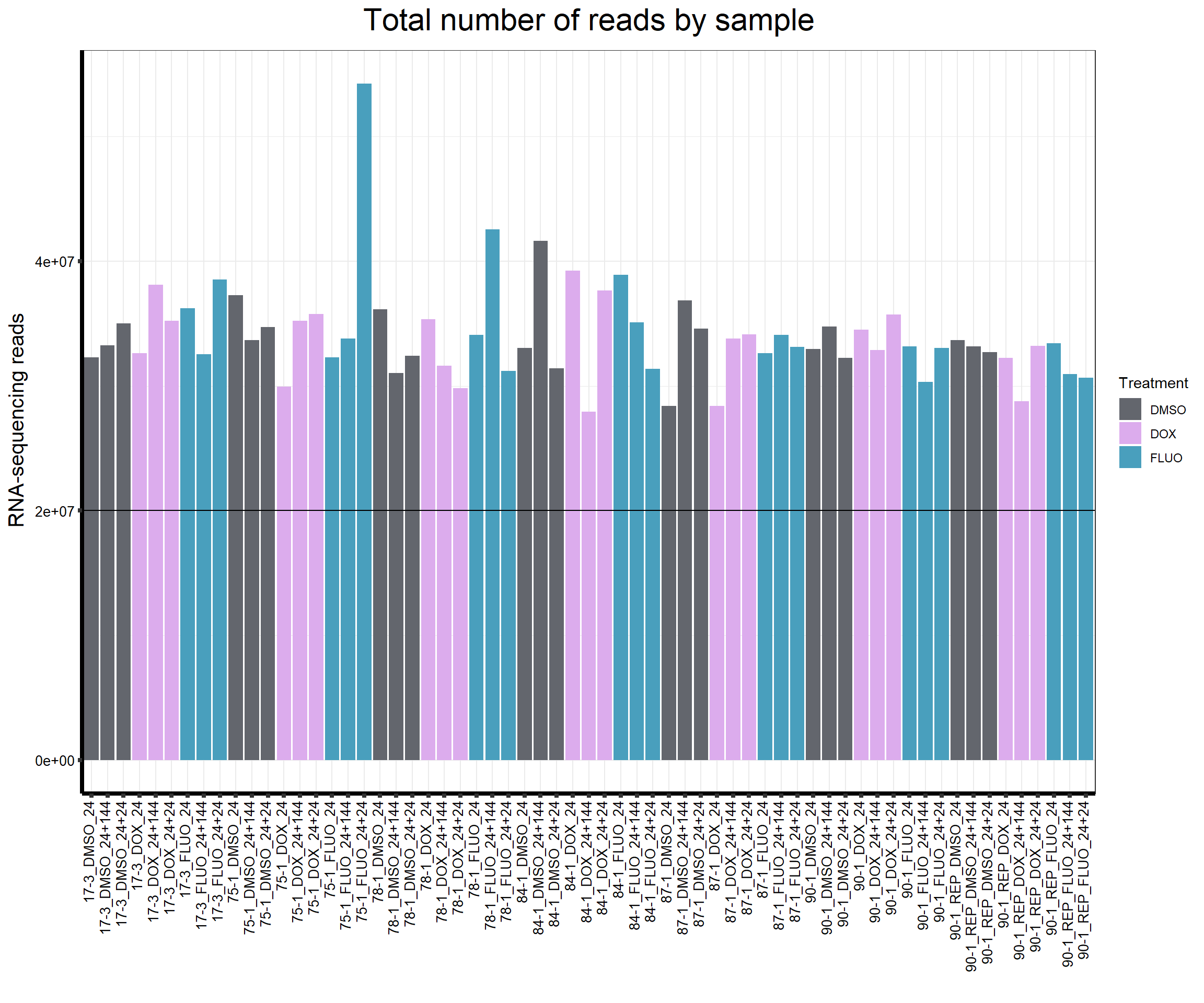

Past versions of "QC checks Raw Counts-1.png"

Version	Author	Date
41aef30	emmapfort	2025-02-27

####Read Counts by Treatment####
fC_AllCounts %>% 
  ggplot(., aes (x =Treatment, y= Total_Align, fill = Treatment))+
  geom_boxplot()+
 scale_fill_manual(values=reads_by_sample)+
  ggtitle(expression("Total number of reads by treatment"))+
  xlab("")+
  ylab(expression("RNA-sequencing reads"))+
  theme_bw()+
  
  theme(plot.title = element_text(size = rel(2), hjust = 0.5),
        axis.title = element_text(size = 15, color = "black"),
        axis.ticks = element_line(linewidth = 1.5),
        axis.line = element_line(linewidth = 1.5),
        axis.text.y = element_text(size =10, color = "black", angle = 0, hjust = 0.8, vjust = 0.5),
        axis.text.x = element_text(size =10, color = "black", angle = 90, hjust = 1, vjust = 0.2),
        #strip.text.x = element_text(size = 15, color = "black", face = "bold"),
        strip.text.y = element_text(color = "white"))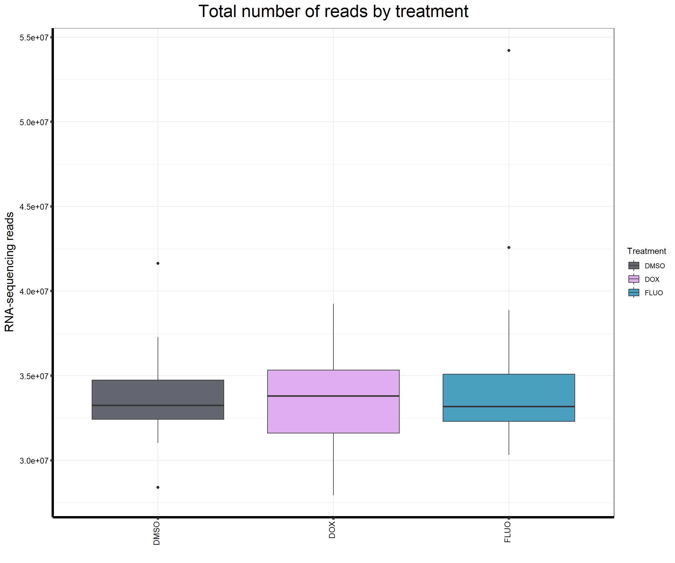

Past versions of "QC checks Raw Counts-2.png"

Version	Author	Date
41aef30	emmapfort	2025-02-27

####Total Reads Per Individual####
fC_AllCounts %>% 
  ggplot(., aes (x =as.factor(Line), y=Total_Align))+
  geom_boxplot(aes(fill=as.factor(Line)))+
 scale_fill_brewer(palette = "Dark2", name = "Individual")+
  ggtitle(expression("Total number of reads by individual"))+
  xlab("")+
  ylab(expression("RNA-sequencing reads"))+
  theme_bw()+

  theme(plot.title = element_text(size = rel(2), hjust = 0.5),
        axis.title = element_text(size = 15, color = "black"),
        axis.ticks = element_line(linewidth = 1.5),
        axis.line = element_line(linewidth = 1.5),
        axis.text.y = element_text(size =10, color = "black", angle = 0, hjust = 0.8, vjust = 0.5),
        axis.text.x = element_text(size =10, color = "black", angle = 0, hjust = 1),
        #strip.text.x = element_text(size = 15, color = "black", face = "bold"),
        strip.text.y = element_text(color = "white"))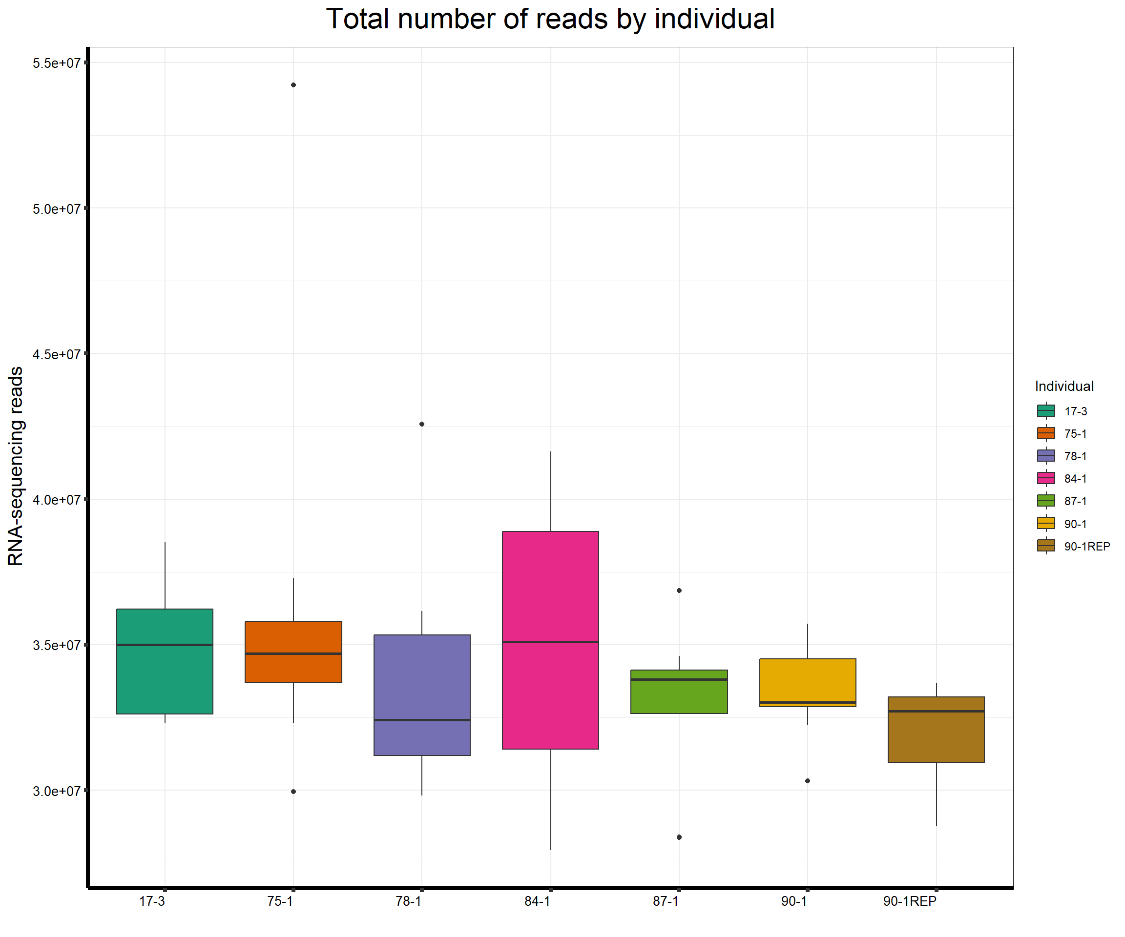

Past versions of "QC checks Raw Counts-3.png"

Version	Author	Date
41aef30	emmapfort	2025-02-27

####Total Mapped Reads Per Drug####

reads_by_sample <- c(tx_col)
fC_AllCounts %>% 
  ggplot(., aes (x = Conditions, y = Assigned_Align, fill = Treatment, group_by = Line))+
  geom_col()+
 geom_hline(aes(yintercept=20000000))+
 scale_fill_manual(values=reads_by_sample)+
  ggtitle(expression("Total number of mapped reads by sample"))+
  xlab("")+
  ylab(expression("RNA-sequencing reads"))+
  theme_bw()+
  theme(plot.title = element_text(size = rel(2), hjust = 0.5),
        axis.title = element_text(size = 15, color = "black"),
        axis.ticks = element_line(linewidth = 1.5),
        axis.line = element_line(linewidth = 1.5),
        axis.text.y = element_text(size =10, color = "black", angle = 0, hjust = 0.8, vjust = 0.5),
        axis.text.x = element_text(size =10, color = "black", angle = 90, hjust = 1, vjust = 0.2),
        #strip.text.x = element_text(size = 15, color = "black", face = "bold"),
        strip.text.y = element_text(color = "white"))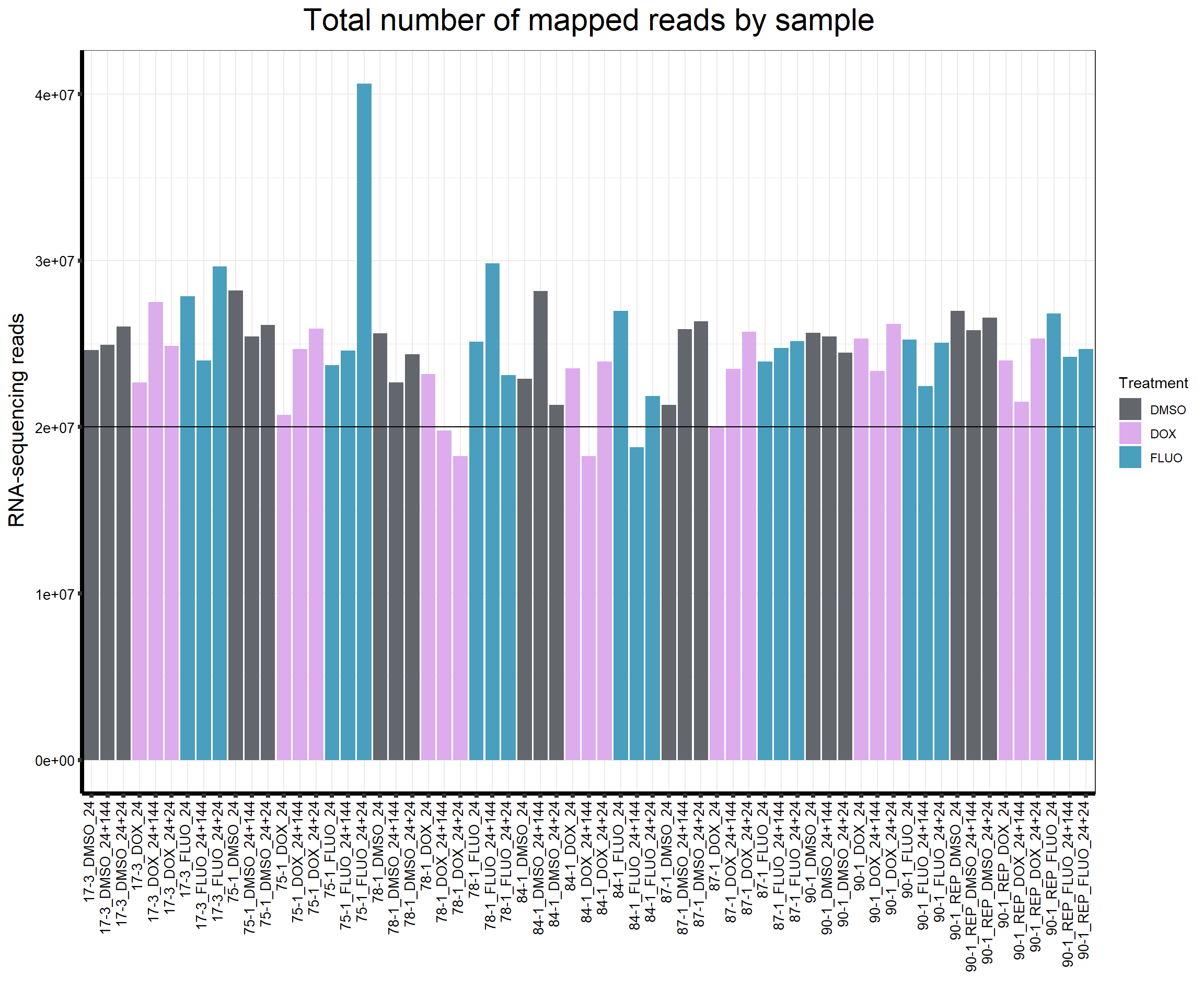

Past versions of "QC checks Raw Counts-4.png"

Version	Author	Date
41aef30	emmapfort	2025-02-27

####Read Counts by Treatment####
fC_AllCounts %>% 
  ggplot(., aes (x =Treatment, y= Assigned_Align, fill = Treatment))+
  geom_boxplot()+
 scale_fill_manual(values=reads_by_sample)+
  ggtitle(expression("Total number of mapped reads by treatment"))+
  xlab("")+
  ylab(expression("RNA-sequencing reads"))+
  theme_bw()+
  
  theme(plot.title = element_text(size = rel(2), hjust = 0.5),
        axis.title = element_text(size = 15, color = "black"),
        axis.ticks = element_line(linewidth = 1.5),
        axis.line = element_line(linewidth = 1.5),
        axis.text.y = element_text(size =10, color = "black", angle = 0, hjust = 0.8, vjust = 0.5),
        axis.text.x = element_text(size =10, color = "black", angle = 90, hjust = 1, vjust = 0.2),
        #strip.text.x = element_text(size = 15, color = "black", face = "bold"),
        strip.text.y = element_text(color = "white"))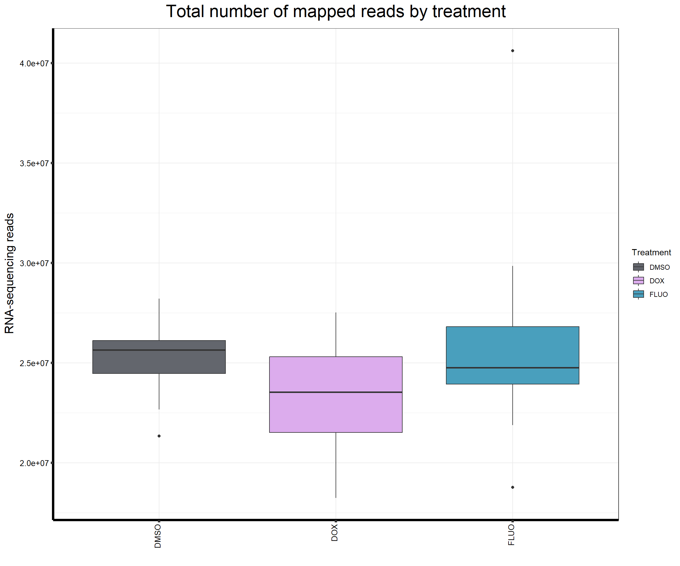

Past versions of "QC checks Raw Counts-5.png"

Version	Author	Date
41aef30	emmapfort	2025-02-27

####Total Reads Per Individual####
fC_AllCounts %>% 
  ggplot(., aes (x =as.factor(Line), y=Assigned_Align))+
  geom_boxplot(aes(fill=as.factor(Line)))+
 scale_fill_brewer(palette = "Dark2", name = "Individual")+
  ggtitle(expression("Total number of mapped reads by individual"))+
  xlab("")+
  ylab(expression("RNA-sequencing reads"))+
  theme_bw()+

  theme(plot.title = element_text(size = rel(2), hjust = 0.5),
        axis.title = element_text(size = 15, color = "black"),
        axis.ticks = element_line(linewidth = 1.5),
        axis.line = element_line(linewidth = 1.5),
        axis.text.y = element_text(size =10, color = "black", angle = 0, hjust = 0.8, vjust = 0.5),
        axis.text.x = element_text(size =10, color = "black", angle = 0, hjust = 1),
        #strip.text.x = element_text(size = 15, color = "black", face = "bold"),
        strip.text.y = element_text(color = "white"))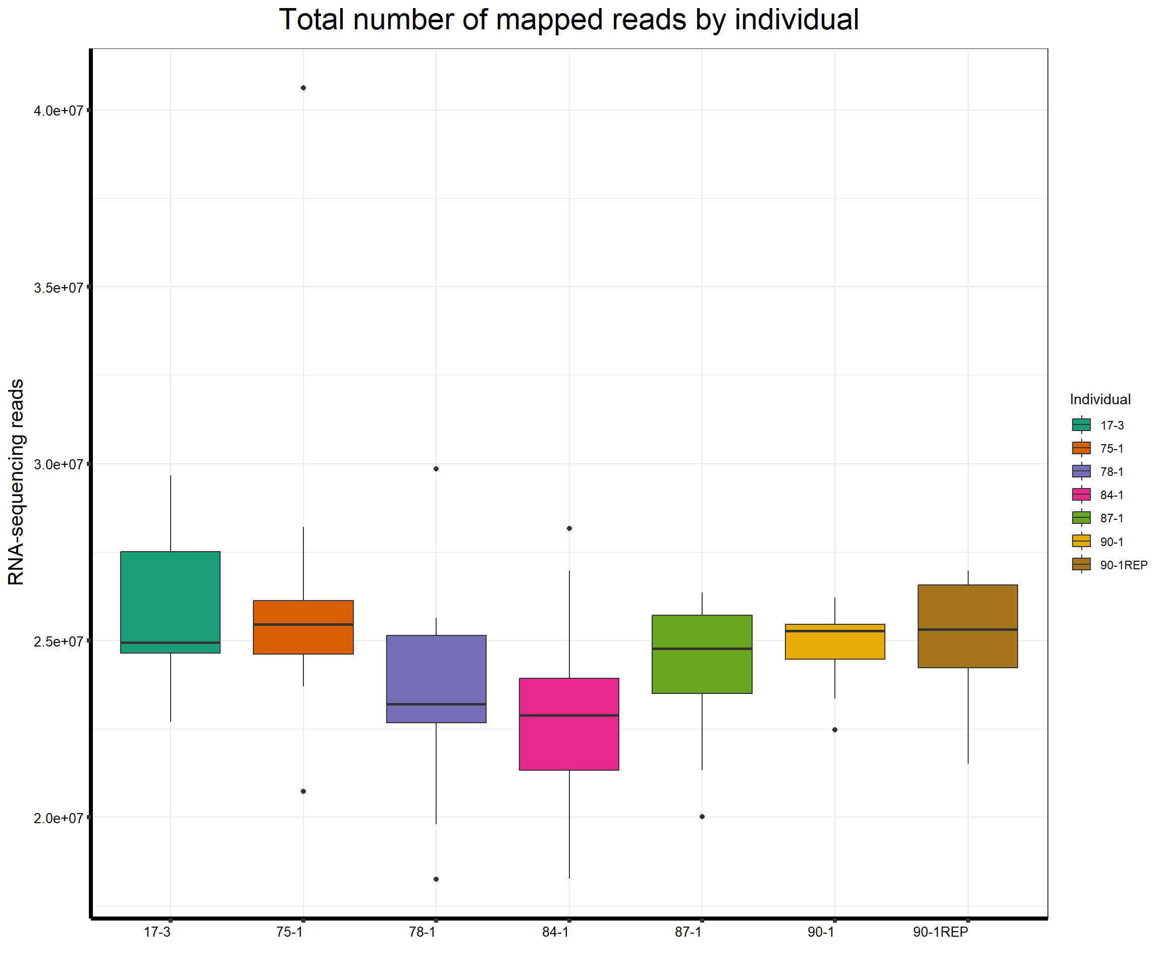

Past versions of "QC checks Raw Counts-6.png"

Version	Author	Date
41aef30	emmapfort	2025-02-27

Now that I’ve made the final full matrix of all samples - 1. convert to log2cpm using cpm 2. filter for lowly expressed reads (rowMeans > 0)

boxplot(fC_Matrix_Full_cpm, xlab = "Conditions", ylab = expression("log"[2]* "counts per million"), ylim= c(-10, 20))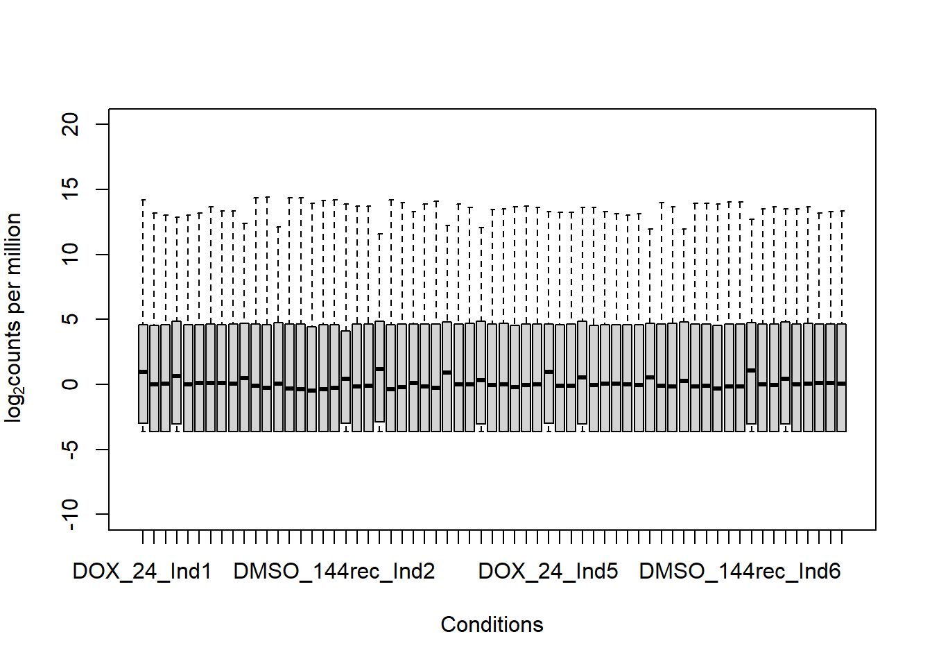

Past versions of "log2cpm Conversion Full Matrix-1.png"

Version	Author	Date
41aef30	emmapfort	2025-02-27

hist(fC_Matrix_Full_cpm, xlab = expression("log" [2]* "counts per million"))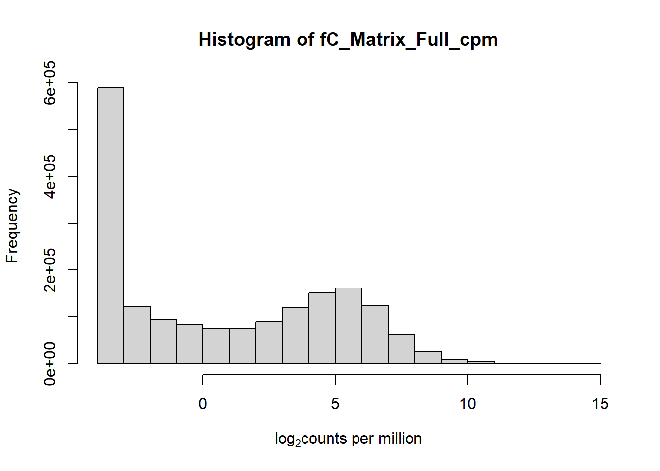

Past versions of "log2cpm Conversion Full Matrix-2.png"

Version	Author	Date
41aef30	emmapfort	2025-02-27

#write this to a csv just in case to save it
#write.csv(fC_Matrix_Full_cpm, "C:/Users/emmap/RDirectory/Recovery_RNAseq/Recovery_RNAseq/featureCounts_Concat_Matrix_AllSamples_cpm_EMP_250210.csv")

#first check the number of variables in the cpm file
dim(fC_Matrix_Full_cpm)
[1] 28395    63
#[1] 28395    63

#now use rowMeans to filter out values with mean < 0 (this means rowMeans > 0 is what I'm left with) for each row/gene in the original file
rowMeans_All <- rowMeans(fC_Matrix_Full_cpm)
fC_Matrix_Full_cpm_filter <- fC_Matrix_Full_cpm[rowMeans_All > 0,]
dim(fC_Matrix_Full_cpm_filter)
[1] 14225    63
#[1] 14225    63

#with this I've filtered out a significant number of rows when filtering after cpm conversion - does this make it more balanced?

hist(fC_Matrix_Full_cpm_filter, 
     main = "Recovery All Individuals log2cpm Filtered", 
        xlab = expression("log"[2]*"counts per million"))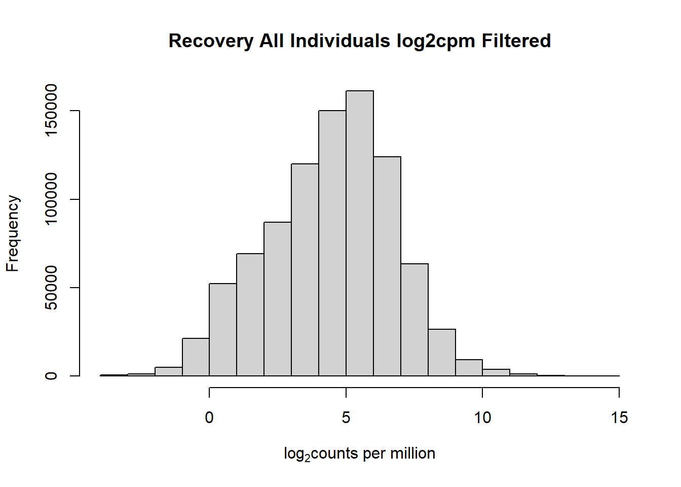

Past versions of "Filter Lowly Expressed Reads All Samples-1.png"

Version	Author	Date
41aef30	emmapfort	2025-02-27

boxplot(fC_Matrix_Full_cpm_filter, 
        main = "Recovery All Individuals log2cpm Filtered", 
        xlab = "Conditions", 
        ylab = expression("log"[2]*"counts per million"),
        ylim = c(-10,15))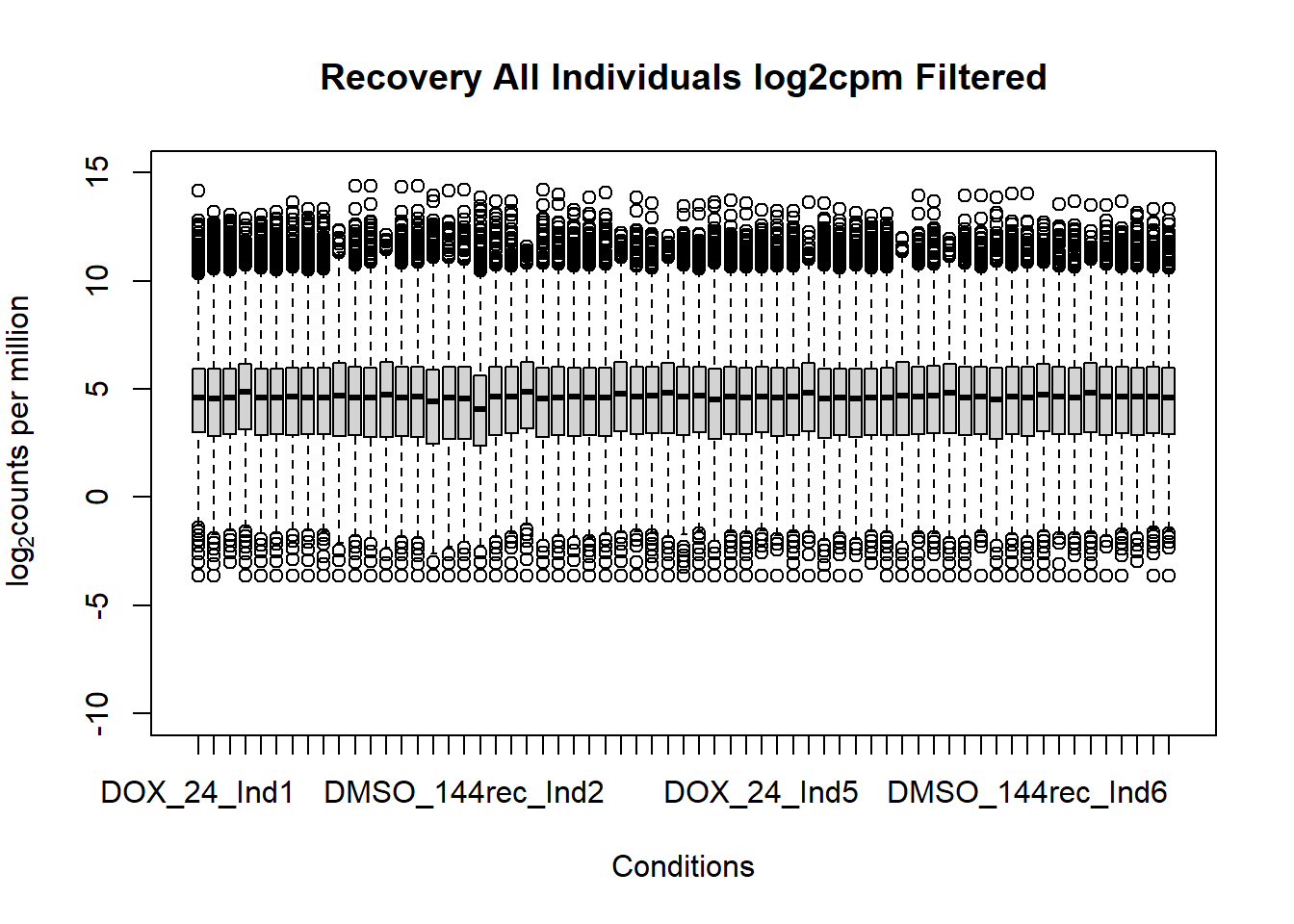

Past versions of "Filter Lowly Expressed Reads All Samples-2.png"

Version	Author	Date
41aef30	emmapfort	2025-02-27

#write this to a csv to save
#write.csv(fC_Matrix_Full_cpm_filter, "C:/Users/emmap/RDirectory/Recovery_RNAseq/Recovery_RNAseq/featureCounts_Concat_Matrix_AllSamples_cpm_filtered_EMP_250210.csv")

####histogram of total counts, unfiltered####
hist(fC_Matrix_Full_cpm, main = "Recovery All Individuals log2cpm Unfiltered",
     xlab = expression("log" [2]* "counts per million"))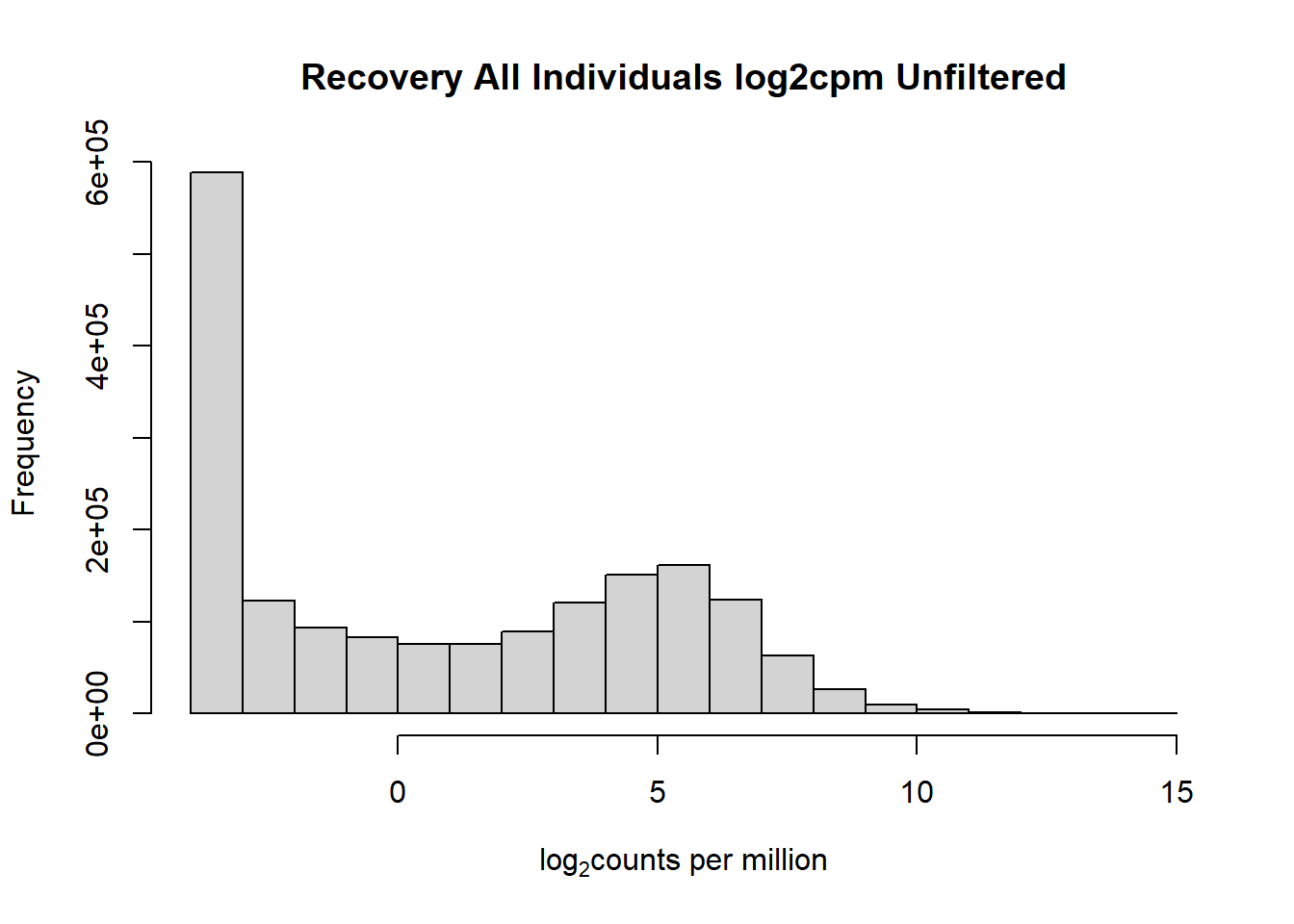

Past versions of "QC Checks Unfiltered vs Filtered Reads-1.png"

Version	Author	Date
41aef30	emmapfort	2025-02-27

####histogram of total counts, filtered####
hist(fC_Matrix_Full_cpm_filter, 
     main = "Recovery All Individuals log2cpm Filtered rowMeans > 0", 
        xlab = expression("log"[2]*"counts per million"))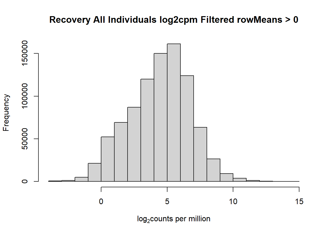

Past versions of "QC Checks Unfiltered vs Filtered Reads-2.png"

Version	Author	Date
41aef30	emmapfort	2025-02-27

####boxplot log2cpm all samples####

boxplot(fC_Matrix_Full_cpm, xlab = "Conditions", ylab = expression("log"[2]* "counts per million"), ylim= c(-10, 20), main = "Boxplots of log2cpm per sample")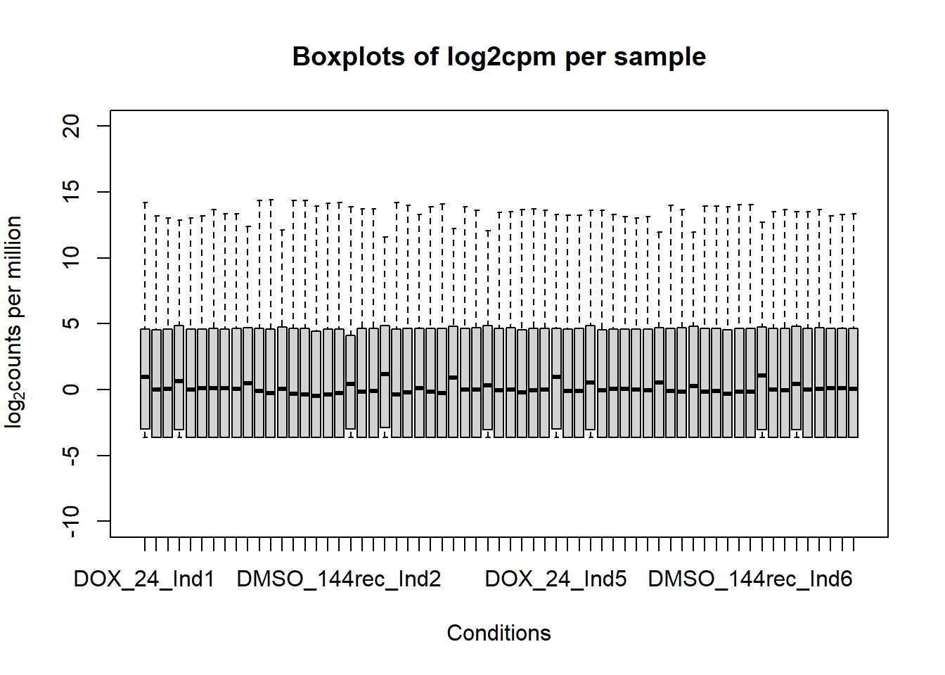

Past versions of "QC Checks Unfiltered vs Filtered Reads-3.png"

Version	Author	Date
41aef30	emmapfort	2025-02-27

####boxplot log2cpm filtered all samples####

boxplot(fC_Matrix_Full_cpm_filter, xlab = "Conditions", ylab = expression("log"[2]* "counts per million"), ylim= c(-10, 20), main = "Boxplots of log2cpm Filtered rowMeans > 0 per sample")

Past versions of "QC Checks Unfiltered vs Filtered Reads-4.png"

Version	Author	Date
41aef30	emmapfort	2025-02-27

Now that I’ve filtered the samples after log2cpm conversion, I can start to make heatmaps and PCA plots to look at my data

After trying and failing to get all three factors on one PCA plot - I will make iterations of each of these with two factors each

Now, I want to update these PCA plots to have treatment and time as the primary variables Individual will be a fill? Or somehow get some numbers labelled on the points.

PCA_data <- fC_Matrix_Full_cpm_filter %>% 
  prcomp(.) %>% 
  t()

PCA_data_test <- (prcomp(t(fC_Matrix_Full_cpm_filter), scale. = TRUE))

####now make an annotation for my PCA####
annot <- data.frame("samples" = colnames(fC_Matrix_Full_cpm_filter)) %>% separate_wider_delim(., cols = samples, names = c("Tx", "Time", "Ind"), delim = "_", cols_remove = FALSE) %>% unite(., col = "Tx_Time", Tx, Time, sep = "_", remove = FALSE)

#combine the prcomp matrix and annotation
annot_PCA_matrix <- PCA_data_test$x %>% cbind(., annot)

#now I can make a graph where I have filled values for individual! I have seven colors for seven individuals
# I have three fill values for three timepoints

#using annotation matrix above as well as annotated PCA matrix (annot_PCA_matrix)

#extra info for colors in the graph (fill parameter)
fill_col_ind <- c("#66C2A5", "#FC8D62", "#1F78B4", "#E78AC3", "#A6D854", "#FFD92A", "#8B3E9B")

fill_col_ind_dark <- c("#003F5C", "#45AE91",  "#58508D", "#BC4099", "#8B3E9B", "#FF6361", "#FF2362")

fill_col_tx <- c("#63666D", "#DCACED", "#499FBD")

#Now I have to switch the fill and color parameters as it's doing the opposite of what I wanted: need individuals to be the outline color (color), and tx to be the inside color (fill)

####PC1/PC2####
annot_PCA_matrix %>% ggplot(., aes(x=PC1, y=PC2, size = 10)) +
  geom_point(aes(color = Ind, shape = Time, fill = Tx)) +
                       scale_shape_manual(values = c(21, 22, 24)) +
  scale_fill_manual(values =  fill_col_tx)+
  scale_color_manual(values = c(fill_col_ind_dark))+
  guides(fill=guide_legend(override.aes=list(shape=21)))+
  guides(color=guide_legend(override.aes=list(shape=21)))+
  guides(fill=guide_legend(override.aes=list(shape=21,fill=fill_col_tx,color=fill_col_tx)))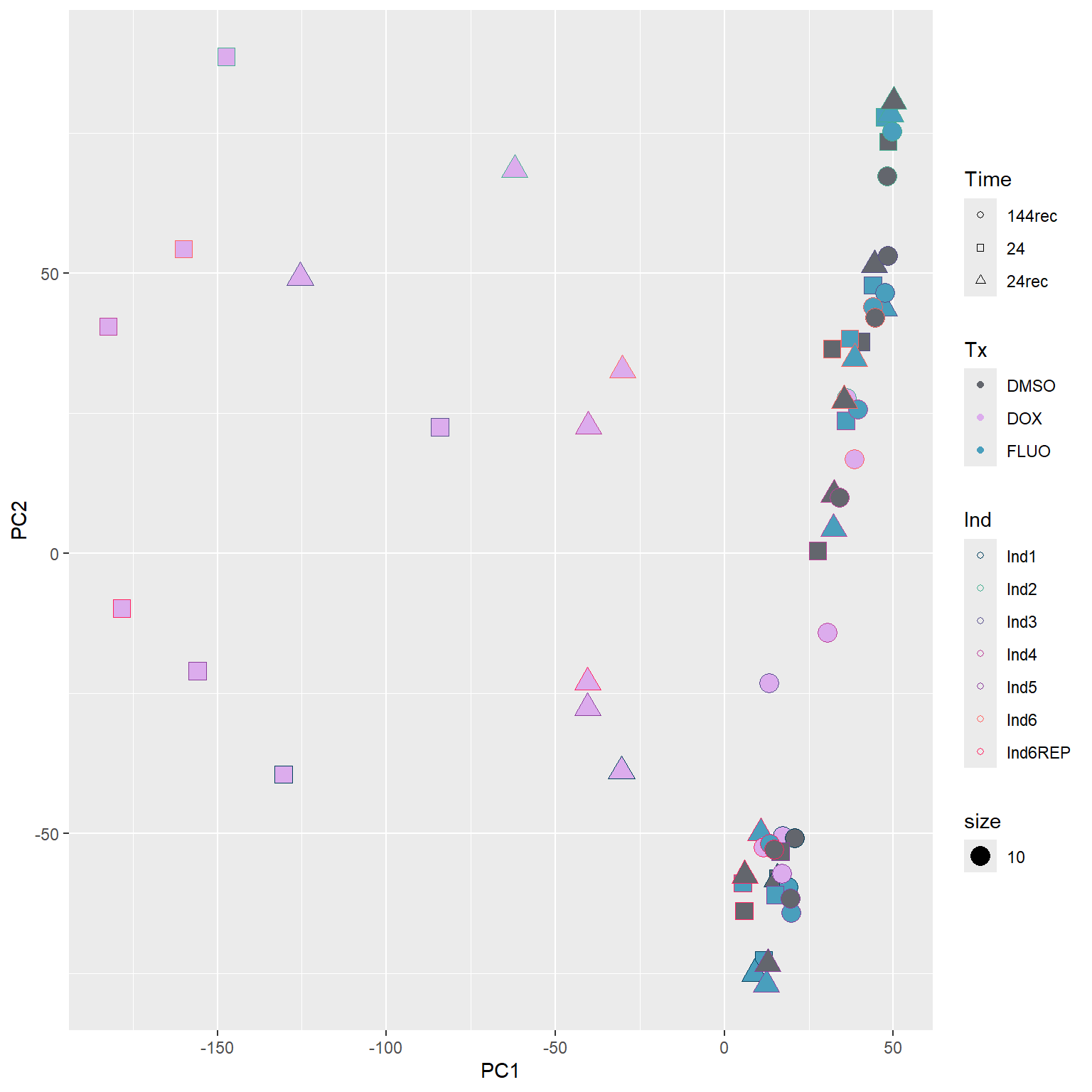

Past versions of "PCA Plots Updated-1.png"

Version	Author	Date
41aef30	emmapfort	2025-02-27

####PC2/PC3####
annot_PCA_matrix %>% ggplot(., aes(x=PC2, y=PC3)) +
  geom_point(aes(color = Ind, shape = Time, fill = Tx, size = 10)) +
                       scale_shape_manual(values = c(21, 22, 24)) +
  scale_fill_manual(values =  fill_col_tx)+
  scale_color_manual(values = c(fill_col_ind_dark))+
  guides(fill=guide_legend(override.aes=list(shape=21)))+
  guides(color=guide_legend(override.aes=list(shape=21)))+
  guides(fill=guide_legend(override.aes=list(shape=21,fill=fill_col_tx,color=fill_col_tx)))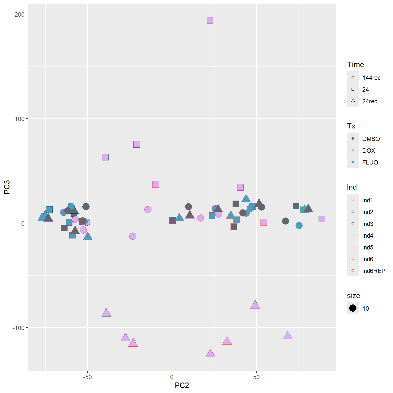

Past versions of "PCA Plots Updated-2.png"

Version	Author	Date
41aef30	emmapfort	2025-02-27

####PC3/PC4####
annot_PCA_matrix %>% ggplot(., aes(x=PC3, y=PC4)) +
  geom_point(aes(color = Ind, shape = Time, fill = Tx, size = 10)) +
                       scale_shape_manual(values = c(21, 22, 24)) +
  scale_fill_manual(values =  fill_col_tx)+
  scale_color_manual(values = c(fill_col_ind_dark))+
  guides(fill=guide_legend(override.aes=list(shape=21)))+
  guides(color=guide_legend(override.aes=list(shape=21)))+
  guides(fill=guide_legend(override.aes=list(shape=21,fill=fill_col_tx,color=fill_col_tx)))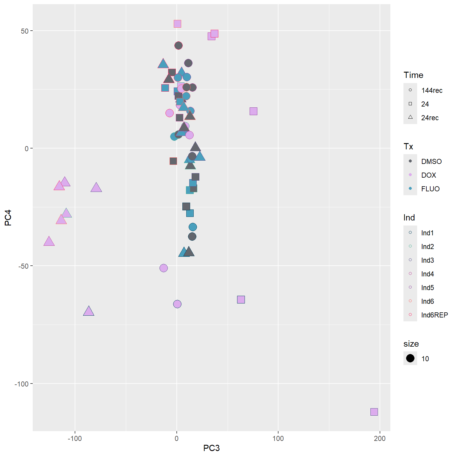

Past versions of "PCA Plots Updated-3.png"

Version	Author	Date
41aef30	emmapfort	2025-02-27

#correlation heatmap for all samples

####PEARSON FILTERED####
fC_Matrix_Full_cpm_filter_pearsoncor <-
  cor(
    fC_Matrix_Full_cpm_filter,
    y = NULL,
    use = "everything",
    method = "pearson"
  )

####SPEARMAN FILTERED####
fC_Matrix_Full_cpm_filter_spearmancor <-
  cor(
    fC_Matrix_Full_cpm_filter,
    y = NULL,
    use = "everything",
    method = "spearman"
  )



#Now let's graph these correlations

pheatmap(fC_Matrix_Full_cpm_filter_pearsoncor, border_color = "black", legend = TRUE, angle_col = 90, display_numbers = FALSE, number_color = "black", fontsize = 12, fontsize_number = 9)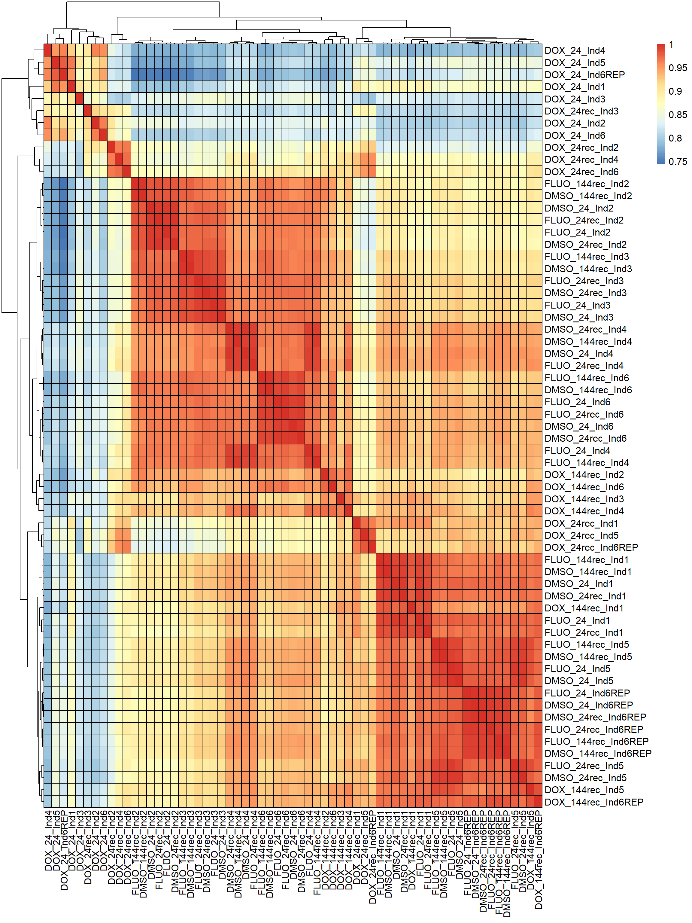

Past versions of "Correlation Heatmaps-1.png"

Version	Author	Date
41aef30	emmapfort	2025-02-27

pheatmap(fC_Matrix_Full_cpm_filter_spearmancor, border_color = "black", legend = TRUE, angle_col = 90, display_numbers = FALSE, number_color = "black", fontsize = 12, fontsize_number = 9)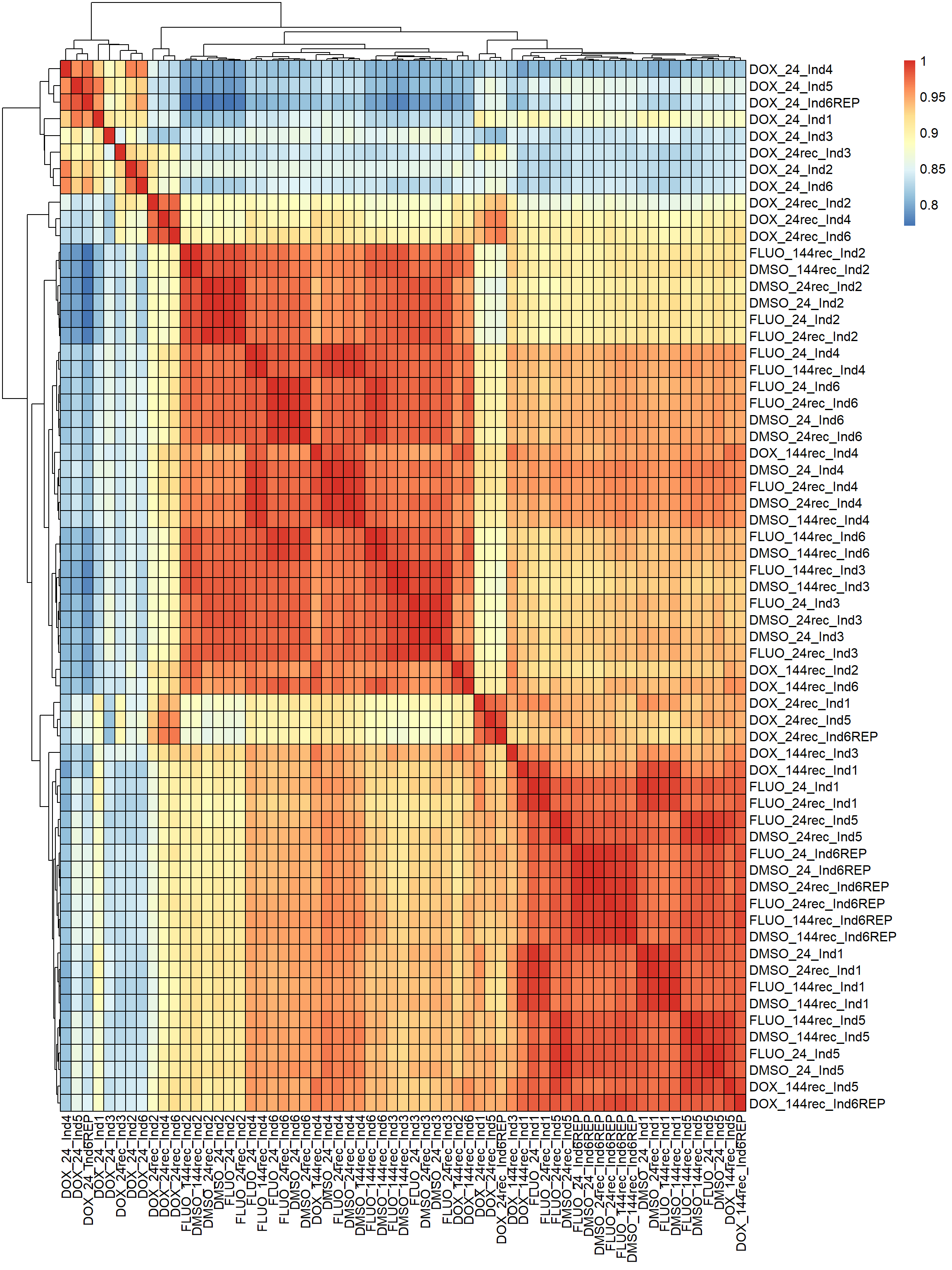

Past versions of "Correlation Heatmaps-2.png"

Version	Author	Date
41aef30	emmapfort	2025-02-27

#now annotate these heatmaps
#Factor 1 - Individual
Individual <- as.factor(c(rep("Ind1", 9), rep("Ind2", 9), rep("Ind3", 9), rep("Ind4", 9), rep("Ind5", 9), rep("Ind6", 9), rep("Ind6REP", 9)))

#Factor 2 - Treatment
tx_factor <- c("DOX", "FLUO", "DMSO")
Tx <- as.factor(c(rep(tx_factor, 21)))
#view(Treatment)

#Factor 3 - Timepoint
time_factor <- c(rep("24", 3), rep("24rec", 3), rep("144rec", 3))
Time <- as.factor(c(rep(time_factor, 7)))

####annotation for colors####
annot_col_hm = list(Tx = c(DOX = "red", FLUO = "blue", DMSO = "black"),
                             Ind = c(Ind1 = "#66C2A5", Ind2 = "#FC8D62", Ind3 = "#1F78B4", Ind4 = "#E78AC3", Ind5 = "#A6D854", Ind6 = "#FFD92A", Ind6REP = "#8B3E9B"),
                             Time = c("24" = "#046A38", "24rec" = "#0050B5", "144rec" = "#B725AD"))

####annotation for values####
annot_list_hm <- data.frame(Individual = as.factor(c(rep("Ind1", 9), rep("Ind2", 9), rep("Ind3", 9), rep("Ind4", 9), rep("Ind5", 9), rep("Ind6", 9), rep("Ind6REP", 9))),
                                               Tx = as.factor(c(rep(tx_factor, 21))), 
                                               Time = as.factor(c(rep(time_factor, 7))))

  
##add in the annotations from above into the dataframe
row.names(annot_list_hm) <- colnames(fC_Matrix_Full_cpm_filter_pearsoncor)
row.names(annot_list_hm) <- colnames(fC_Matrix_Full_cpm_filter_spearmancor)

####ANNOTATED HEATMAPS####
pheatmap(fC_Matrix_Full_cpm_filter_pearsoncor, border_color = "black", legend = TRUE, angle_col = 90, display_numbers = FALSE, number_color = "black", fontsize = 10, fontsize_number = 5, annotation_col = annot_list_hm, annotation_colors = annot_col_hm)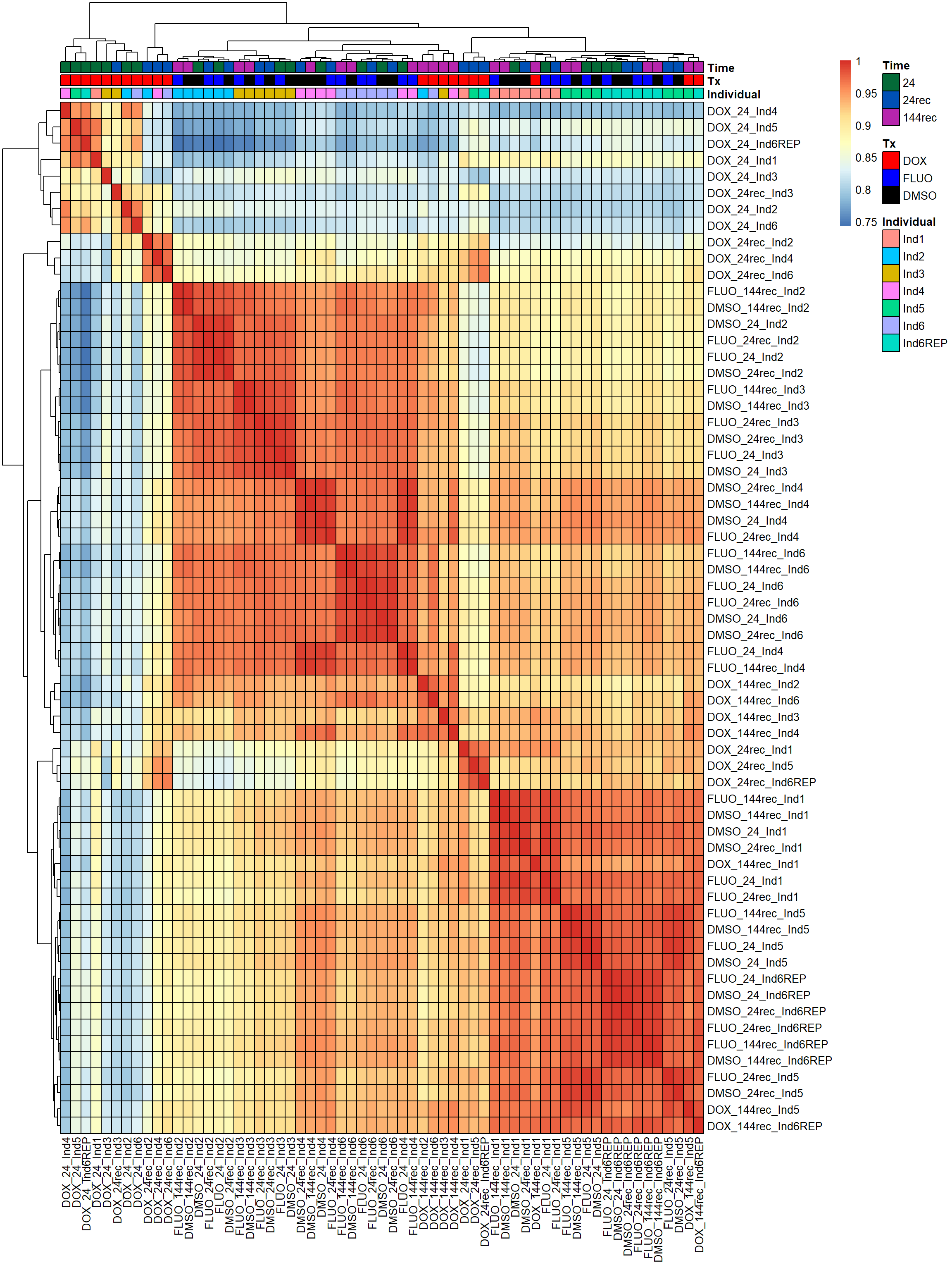

Past versions of "Correlation Heatmaps-3.png"

Version	Author	Date
41aef30	emmapfort	2025-02-27

pheatmap(fC_Matrix_Full_cpm_filter_spearmancor, border_color = "black", legend = TRUE, angle_col = 90, display_numbers = FALSE, number_color = "black", fontsize = 10, fontsize_number = 5, annotation_col = annot_list_hm, annotation_colors = annot_col_hm)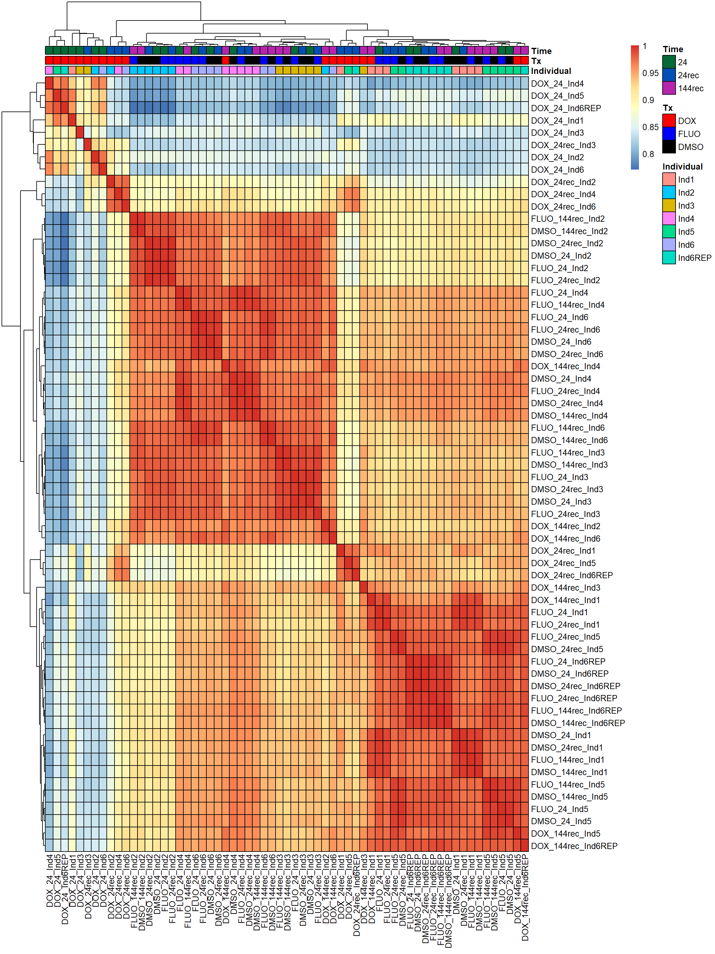

Past versions of "Correlation Heatmaps-4.png"

Version	Author	Date
41aef30	emmapfort	2025-02-27

Now that I’ve finalized my QC checks, I will go ahead and begin the differential expression analysis pipeline.

# group <- c(rep(c(1, 2, 3, 4, 5, 6, 7, 8, 9), 6))
# group <- factor(group, levels = c("1", "2", "3", "4", "5", "6", "7", "8", "9"))


####rowMeans > 0 Filtering####
rowMeans_DE <- rowMeans(counts_DE)
counts_DE_filter <- counts_DE[rowMeans_DE > 0,]
dim(counts_DE_filter)
[1] 26445    54

group_1 <- rep(c("DOX_24","FLUO_24",
                                "DMSO_24",
                                "DOX_24rec",
                                "FLUO_24rec",
                                "DMSO_24rec",
                                "DOX_144rec",
                                "FLUO_144rec",
                                "DMSO_144rec"), 6)

dge <- DGEList.data.frame(counts = counts_DE_filter, group = group_1, genes = row.names(counts_DE_filter))

#check the inital file before norm factors are calculated
#dge$samples

#calculate the normalization factors with method TMM
dge_calc <- calcNormFactors(dge, method = "TMM")

#check final file after norm calculation
#dge_calc$samples

#after calculating norm factors, that column was changed.

#View(dge_calc)

#Pull out factors
snames <- data.frame("samples" = colnames(dge_calc)) %>% separate_wider_delim(., cols = samples, names = c("Treatment", "Time", "Individual"), delim = "_", cols_remove = FALSE)

#snames_list <- as.list(snames)

snames_time <- snames$Time
snames_tx <- snames$Treatment
snames_ind <- snames$Individual

#Create my model matrix
mm_r <- model.matrix(~0 + group_1)

p <- voom(dge_calc$counts, mm_r, plot = TRUE)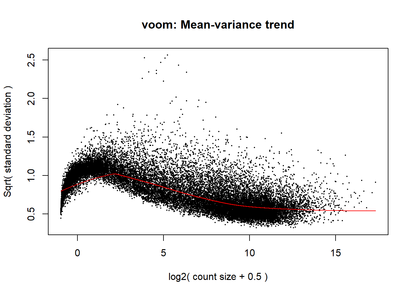

Past versions of "Differential Expression Analysis filtering rowMeans greater than 0-1.png"

Version	Author	Date
41aef30	emmapfort	2025-02-27

corfit <- duplicateCorrelation(p, mm_r, block = snames_ind)

v <- voom(dge_calc$counts, mm_r, block = snames_ind, correlation = corfit$consensus)

fit <- lmFit(v, mm_r, block = snames_ind, correlation = corfit$consensus)

#make sure to check which order the columns are in - otherwise they won't match right (it was moved into alphabetical and number order)
colnames(mm_r) <- c("DMSO_144rec","DMSO_24","DMSO_24rec","DOX_144rec","DOX_24","DOX_24rec","FLUO_144rec","FLUO_24","FLUO_24rec")

cm_r <- makeContrasts(
        V.D24 = DOX_24 - DMSO_24,
        V.F24 = FLUO_24 - DMSO_24,
        V.D24r = DOX_24rec - DMSO_24rec,
        V.F24r = FLUO_24rec - DMSO_24rec,
        V.D144r = DOX_144rec - DMSO_144rec,
        V.F144r = FLUO_144rec - DMSO_144rec,
        levels = mm_r
)

vfit_r <- lmFit(p, mm_r)
vfit_r <- contrasts.fit(vfit_r, contrasts = cm_r)

efit2 <- eBayes(vfit_r)

results = decideTests(efit2)
summary(results)
       V.D24 V.F24 V.D24r V.F24r V.D144r V.F144r
Down    4567     0   2083      0     288       0
NotSig 14521 26445  16339  26445   25296   26445
Up      7357     0   8023      0     861       0
#inbuilt annotation results rowMeans >0
#         V.D24 V.F24 V.D24r V.F24r V.D144r V.F144r
# Down    4567     0   2083      0     288       0
# NotSig 14521 26445  16339  26445   25296   26445
# Up      7357     0   8023      0     861       0

## have no DE genes detected for 5FU, only DOX


####plot your voom####
voom_plot <- voom(dge_calc, mm_r, plot = TRUE)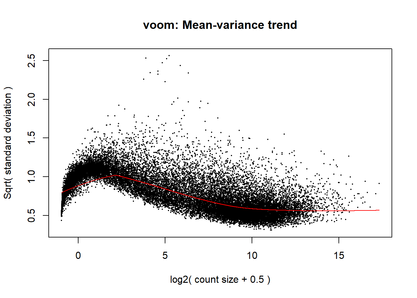

Past versions of "Differential Expression Analysis filtering rowMeans greater than 0-2.png"

Version	Author	Date
41aef30	emmapfort	2025-02-27

The voom plot for this with rowMeans > 0 has a dip in the front, meaning that there is likely some noise left over in my data. I am going to filter a bit stricter at rowMeans > 1 with the same process as above.

####rowMeans >1####
rowMeans_DE <- rowMeans(counts_DE)
counts_DE_filter1 <- counts_DE[rowMeans_DE > 1,]
dim(counts_DE_filter1)
[1] 20443    54


dge1 <- DGEList.data.frame(counts = counts_DE_filter1, group = group_1, genes = row.names(counts_DE_filter1))

#check the inital file before norm factors are calculated
#dge1$samples

#calculate the normalization factors with method TMM
dge1_calc <- calcNormFactors(dge1, method = "TMM")

#check final file after norm calculation
#dge1_calc$samples

#View(dge1_calc)

#Pull out factors
snames1 <- data.frame("samples" = colnames(dge1_calc)) %>% separate_wider_delim(., cols = samples, names = c("Treatment", "Time", "Individual"), delim = "_", cols_remove = FALSE)

#snames_list <- as.list(snames)

snames1_time <- snames1$Time
snames1_tx <- snames1$Treatment
snames1_ind <- snames1$Individual

#Create my model matrix
mm_r1 <- model.matrix(~0 + group_1)

p1 <- voom(dge1_calc$counts, mm_r1, plot = TRUE)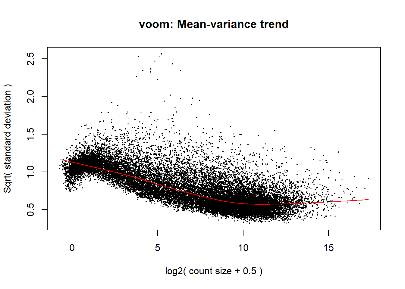

Past versions of "Differential Expression Analysis filtering rowMeans greater than 1-1.png"

Version	Author	Date
41aef30	emmapfort	2025-02-27

corfit1 <- duplicateCorrelation(p1, mm_r1, block = snames1_ind)

v1 <- voom(dge1_calc$counts, mm_r1, block = snames1_ind, correlation = corfit1$consensus)

fit1 <- lmFit(v1, mm_r1, block = snames1_ind, correlation = corfit1$consensus)

#make sure to check which order the columns are in - otherwise they won't match right (it was moved into alphabetical and number order)
colnames(mm_r1) <- c("DMSO_144rec","DMSO_24","DMSO_24rec","DOX_144rec","DOX_24","DOX_24rec","FLUO_144rec","FLUO_24","FLUO_24rec")

cm_r1 <- makeContrasts(
        V.D24 = DOX_24 - DMSO_24,
        V.F24 = FLUO_24 - DMSO_24,
        V.D24r = DOX_24rec - DMSO_24rec,
        V.F24r = FLUO_24rec - DMSO_24rec,
        V.D144r = DOX_144rec - DMSO_144rec,
        V.F144r = FLUO_144rec - DMSO_144rec,
        levels = mm_r1
)

vfit_r1 <- lmFit(p1, mm_r1)
vfit_r1 <- contrasts.fit(vfit_r1, contrasts = cm_r1)

efit4 <- eBayes(vfit_r1)

results1 = decideTests(efit4)
summary(results1)
       V.D24 V.F24 V.D24r V.F24r V.D144r V.F144r
Down    4640     0   2120      0     263       0
NotSig  9460 20443  11485  20443   19838   20443
Up      6343     0   6838      0     342       0
#inbuilt annotation results rowMeans >0
#         V.D24 V.F24 V.D24r V.F24r V.D144r V.F144r
# Down    4567     0   2083      0     288       0
# NotSig 14521 26445  16339  26445   25296   26445
# Up      7357     0   8023      0     861       0

## have no DE genes detected for 5FU, only DOX


####plot your voom####
voom_plot1 <- voom(dge1_calc, mm_r1, plot = TRUE)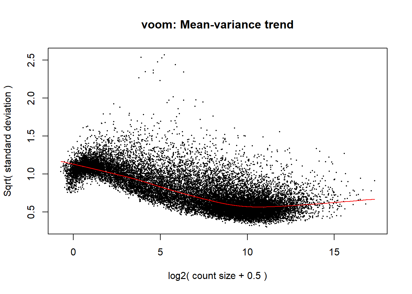

Past versions of "Differential Expression Analysis filtering rowMeans greater than 1-2.png"

Version	Author	Date
41aef30	emmapfort	2025-02-27

This looks much better! No more noise in the front. I could potentially filter at rowMeans >0.5, but I will leave that for now.

Now I can go ahead and make toptables for safekeeping and later analysis

top.table_V.D24 <- topTable(fit = efit4, coef = "V.D24", number = nrow(dge_calc), adjust.method = "BH", p.value = 1, sort.by = "none")
head(top.table_V.D24)

top.table_V.F24 <- topTable(fit = efit4, coef = "V.F24", number = nrow(dge_calc), adjust.method = "BH", p.value = 1, sort.by = "none")
head(top.table_V.F24)

top.table_V.D24r <- topTable(fit = efit4, coef = "V.D24r", number = nrow(dge_calc), adjust.method = "BH", p.value = 1, sort.by = "none")
head(top.table_V.D24r)

top.table_V.F24r <- topTable(fit = efit4, coef = "V.F24r", number = nrow(dge_calc), adjust.method = "BH", p.value = 1, sort.by = "none")
head(top.table_V.F24r)

top.table_V.D144r <- topTable(fit = efit4, coef = "V.D144r", number = nrow(dge_calc), adjust.method = "BH", p.value = 1, sort.by = "none")
head(top.table_V.D144r)

top.table_V.F144r <- topTable(fit = efit4, coef = "V.F144r", number = nrow(dge_calc), adjust.method = "BH", p.value = 1, sort.by = "none")
head(top.table_V.F144r)

Volcano Plots

generate_volcano_plot <- function(toptable, title) {
  
  # Add Significance Labels
  toptable$Significance <- "Not Significant"
  toptable$Significance[toptable$logFC > 0 & toptable$adj.P.Val < 0.05] <- "Upregulated"
  toptable$Significance[toptable$logFC < 0 & toptable$adj.P.Val < 0.05] <- "Downregulated"

  # Generate Volcano Plot
  ggplot(toptable, aes(x = logFC, y = -log10(P.Value), color = Significance)) +
    geom_point(alpha = 0.4, size = 2) + 
    scale_color_manual(values = c("Downregulated" = "red", "Upregulated" = "blue", "Not Significant" = "gray")) +
    xlim(-5, 5) +
    labs(title = title, x = "log2 Fold Change", y = "-log10 P-value") +
    theme(legend.position = "none", 
          plot.title = element_text(size = rel(1.5), hjust = 0.5),
          axis.title = element_text(size = rel(1.25))) +
    theme_bw()
}

#now that I've made a function, I can make volcano plots for each of my comparisons (6 total)

volcano_plots <- list(
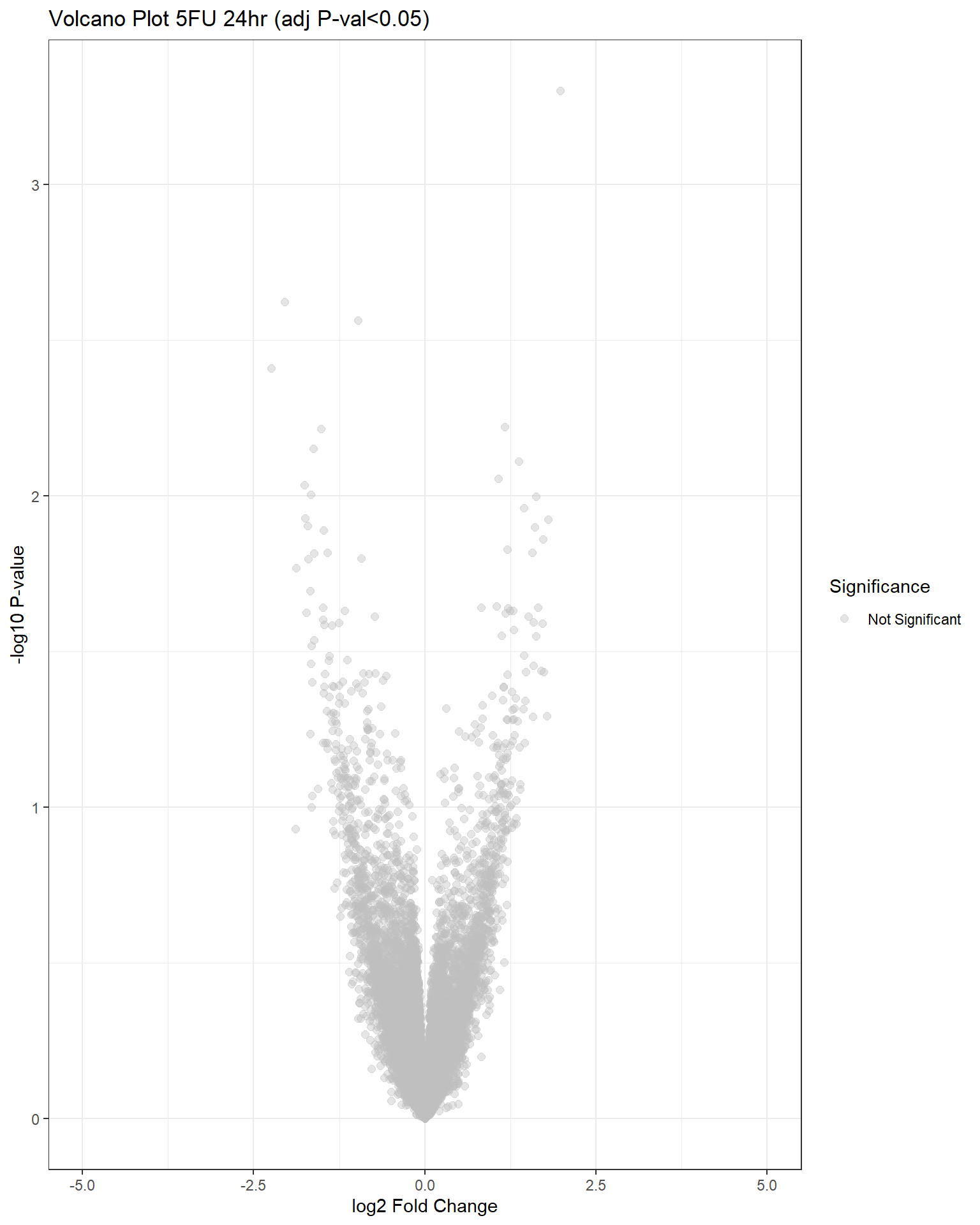
  "V.D24" = generate_volcano_plot(top.table_V.D24, "Volcano Plot DOX 24hr (adj P-val<0.05)"),
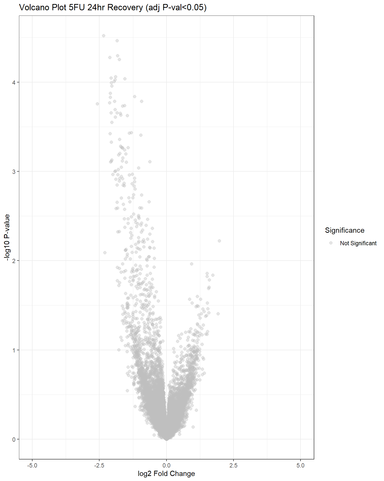
  "V.F24" = generate_volcano_plot(top.table_V.F24, "Volcano Plot 5FU 24hr (adj P-val<0.05)"),
  "V.D24r" = generate_volcano_plot(top.table_V.D24r, "Volcano Plot DOX 24hr Recovery (adj P-val<0.05)"),
  "V.F24r" = generate_volcano_plot(top.table_V.F24r, "Volcano Plot 5FU 24hr Recovery (adj P-val<0.05)"),
  "V.D144r" = generate_volcano_plot(top.table_V.D144r, "Volcano Plot DOX 6d Recovery (adj P-val<0.05)"),
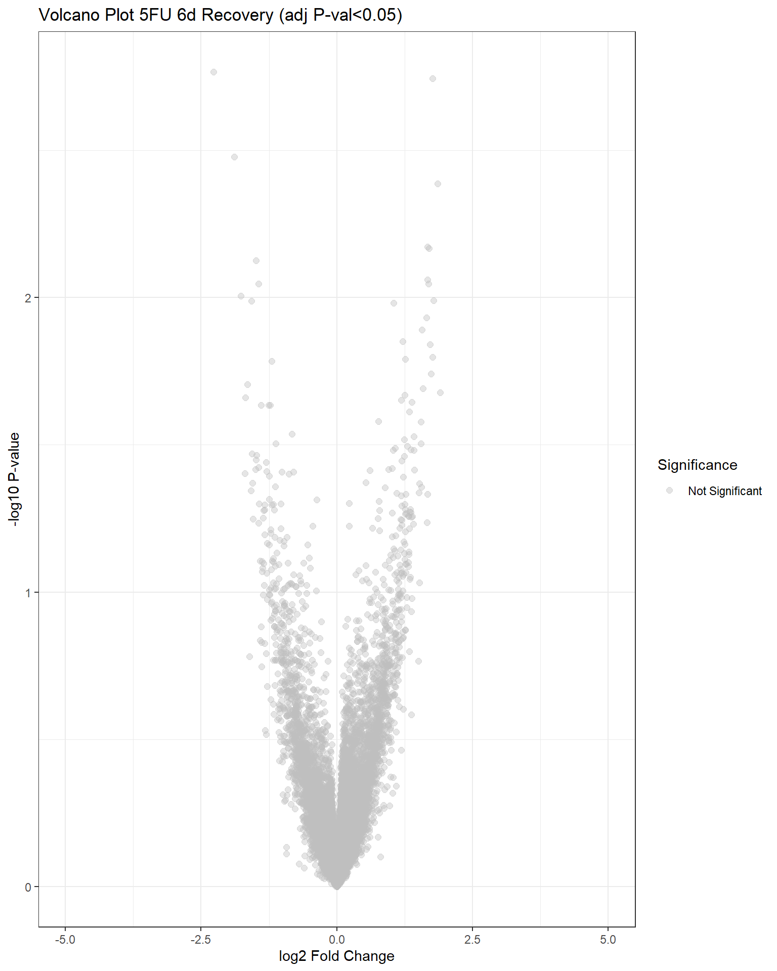
  "V.F144r" = generate_volcano_plot(top.table_V.F144r, "Volcano Plot 5FU 6d Recovery (adj P-val<0.05)")
)

# Display each volcano plot
for (plot_name in names(volcano_plots)) {
  print(volcano_plots[[plot_name]])
}
Warning: Removed 344 rows containing missing values or values outside the scale range
(`geom_point()`).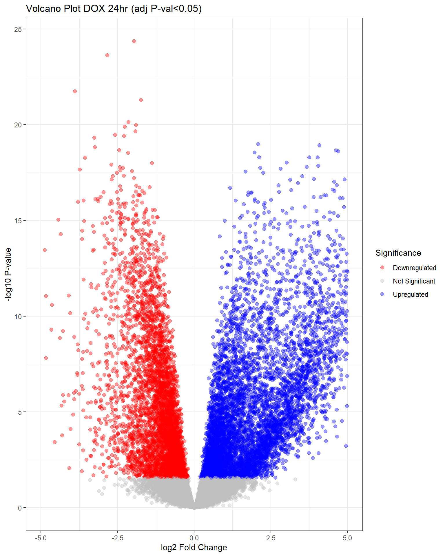

Past versions of "Volcano Plots from Pairwise Gene Analysis-1.png"

Version	Author	Date
41aef30	emmapfort	2025-02-27

Past versions of "Volcano Plots from Pairwise Gene Analysis-2.png"

Version	Author	Date
41aef30	emmapfort	2025-02-27

Warning: Removed 66 rows containing missing values or values outside the scale range
(`geom_point()`).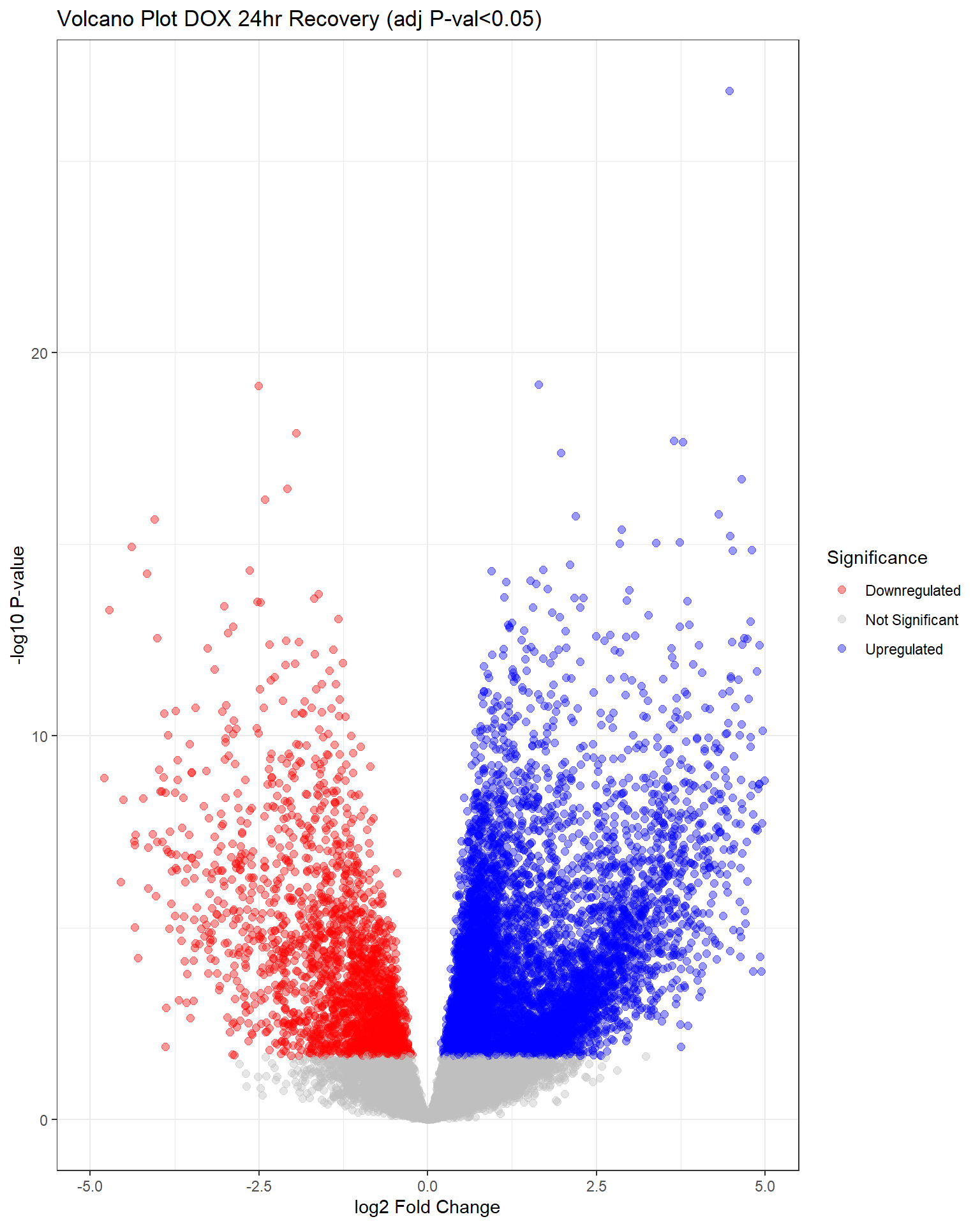

Past versions of "Volcano Plots from Pairwise Gene Analysis-3.png"

Version	Author	Date
41aef30	emmapfort	2025-02-27

Past versions of "Volcano Plots from Pairwise Gene Analysis-4.png"

Version	Author	Date
41aef30	emmapfort	2025-02-27

Warning: Removed 23 rows containing missing values or values outside the scale range
(`geom_point()`).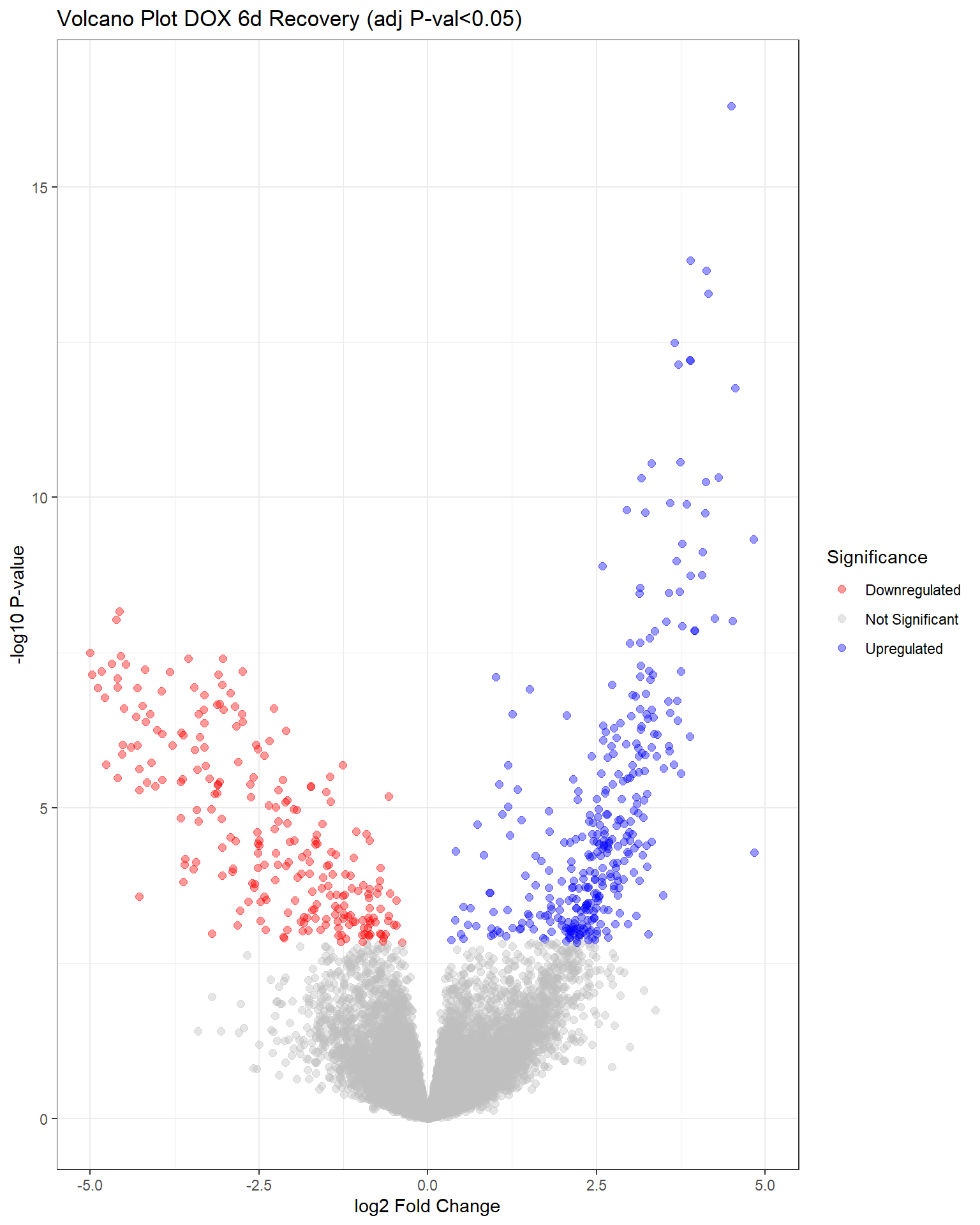

Past versions of "Volcano Plots from Pairwise Gene Analysis-5.png"

Version	Author	Date
41aef30	emmapfort	2025-02-27

Past versions of "Volcano Plots from Pairwise Gene Analysis-6.png"

Version	Author	Date
41aef30	emmapfort	2025-02-27

Now that I’ve gone through and figured out the basics of DE - let’s remove unwanted variation using ruv This uses my replicates to figure out covariates in the data and remove variation occurring due to batch effects or other effects We’re seeing a batch effect from RNA extraction (all RNAseq library prep done in a single batch) occurring here in PCA and cor. heatmaps rather than individuals clustering together.

# #counts need to be integer values and in a numeric matrix for ruv
# counts_DE_matrix <- as.matrix(counts_DE_filter1)
# dim(counts_DE_matrix)
# #[1] 20443    54 - new inbuilt
# #this does NOT contain the replicate samples, save for later
# 
# ##this file contains the replicates that I can pull from
# fC_Matrix_cpm_filter_ruv <- as.matrix (fC_Matrix_Full_cpm_filter)
# 
# #create a matrix specifying the replicates
# reps <- as.data.frame(fC_Matrix_Full_cpm_filter) %>%
#   dplyr::select(contains("Ind6"))
# dim(reps)
# #[1] 14225    18
# reps_mat <- as.matrix(reps)
# 
# #using the documentation do this:
# #controls: gene-by-sample numeric matrix containing counts
# controls <- rownames(fC_Matrix_Full_cpm_filter)
# 
# #I have replicates for Individual 6, which I can compare using this method
# #They are matched as following:
# ##col46:55, 47:56, 48:57, 49:58, 50:59, 51:60, 52:61, 53:62, 54:63
# ###this is the scIdx argument for reps, the cIdx argument is for genes
# #differences <- matrix(data = c(1, 10, 2, 11, 3, 12, 4, 13, 5, 14, 6, 15, 7, 16, 8, 17, 9, 18), byrow = TRUE, nrow = 9)
# differences_full <- matrix(data = c(46, 55, 47, 56, 48 , 57, 49, 58, 50 , 59, 51, 60, 52, 61, 53, 62, 54, 63), byrow = TRUE, nrow = 9)
# 
# 
# signature(x = "matrix", cIdx = "ANY", k = "numeric", scIdx = "matrix")
# 
# 
# seqRUVs <- RUVs(rep, controls, k=3, differences_full, isLog = TRUE)
# 
# pData(counts_DE)
# head(seqRUVs)
# 
# 
# ###now try putting this in your matrix?
# design <- model.matrix(~0 + group_1, seqRUVs)
# 
# 
# 
# 
# ####try it exactly like the documentation and filter afterwards?####
# genes <- rownames(fC_Matrix_Full)[grep("^"), rownames(fC_Matrix_Full)]
# spikes <- rownames()
# 
# ####leaving off here EMP 25/02/26####

Session information

sessionInfo()

R version 4.4.2 (2024-10-31 ucrt)
Platform: x86_64-w64-mingw32/x64
Running under: Windows 11 x64 (build 22000)

Matrix products: default


locale:
[1] LC_COLLATE=English_United States.utf8 
[2] LC_CTYPE=English_United States.utf8   
[3] LC_MONETARY=English_United States.utf8
[4] LC_NUMERIC=C                          
[5] LC_TIME=English_United States.utf8    

time zone: America/Chicago
tzcode source: internal

attached base packages:
[1] stats4    stats     graphics  grDevices utils     datasets  methods  
[8] base     

other attached packages:
 [1] RUVSeq_1.40.0               EDASeq_2.40.0              
 [3] ShortRead_1.64.0            GenomicAlignments_1.42.0   
 [5] SummarizedExperiment_1.36.0 MatrixGenerics_1.18.1      
 [7] matrixStats_1.4.1           Rsamtools_2.22.0           
 [9] GenomicRanges_1.58.0        Biostrings_2.74.0          
[11] GenomeInfoDb_1.42.3         XVector_0.46.0             
[13] IRanges_2.40.0              S4Vectors_0.44.0           
[15] BiocParallel_1.40.0         biomaRt_2.62.1             
[17] RColorBrewer_1.1-3          Cormotif_1.52.0            
[19] affy_1.84.0                 Biobase_2.66.0             
[21] BiocGenerics_0.52.0         PCAtools_2.18.0            
[23] ggrepel_0.9.6               ggfortify_0.4.17           
[25] pheatmap_1.0.12             edgeR_4.4.0                
[27] limma_3.62.1                readxl_1.4.3               
[29] edgebundleR_0.1.4           lubridate_1.9.3            
[31] forcats_1.0.0               stringr_1.5.1              
[33] dplyr_1.1.4                 purrr_1.0.2                
[35] readr_2.1.5                 tidyr_1.3.1                
[37] tidyverse_2.0.0             tibble_3.2.1               
[39] hrbrthemes_0.8.7            reshape2_1.4.4             
[41] ggplot2_3.5.1               workflowr_1.7.1            

loaded via a namespace (and not attached):
  [1] later_1.4.1               BiocIO_1.16.0            
  [3] bitops_1.0-9              filelock_1.0.3           
  [5] R.oo_1.27.0               cellranger_1.1.0         
  [7] preprocessCore_1.68.0     XML_3.99-0.18            
  [9] lifecycle_1.0.4           httr2_1.1.0              
 [11] pwalign_1.2.0             rprojroot_2.0.4          
 [13] vroom_1.6.5               MASS_7.3-61              
 [15] processx_3.8.5            lattice_0.22-6           
 [17] magrittr_2.0.3            sass_0.4.9               
 [19] rmarkdown_2.29            jquerylib_0.1.4          
 [21] yaml_2.3.10               httpuv_1.6.15            
 [23] cowplot_1.1.3             DBI_1.2.3                
 [25] abind_1.4-8               zlibbioc_1.52.0          
 [27] R.utils_2.12.3            RCurl_1.98-1.16          
 [29] rappdirs_0.3.3            git2r_0.35.0             
 [31] gdtools_0.4.1             GenomeInfoDbData_1.2.13  
 [33] irlba_2.3.5.1             dqrng_0.4.1              
 [35] DelayedMatrixStats_1.28.1 codetools_0.2-20         
 [37] DelayedArray_0.32.0       xml2_1.3.6               
 [39] tidyselect_1.2.1          farver_2.1.2             
 [41] UCSC.utils_1.2.0          ScaledMatrix_1.14.0      
 [43] BiocFileCache_2.14.0      jsonlite_1.8.9           
 [45] systemfonts_1.1.0         tools_4.4.2              
 [47] progress_1.2.3            Rcpp_1.0.13-1            
 [49] glue_1.8.0                gridExtra_2.3            
 [51] Rttf2pt1_1.3.12           SparseArray_1.6.0        
 [53] xfun_0.49                 withr_3.0.2              
 [55] BiocManager_1.30.25       fastmap_1.2.0            
 [57] latticeExtra_0.6-30       callr_3.7.6              
 [59] digest_0.6.37             rsvd_1.0.5               
 [61] timechange_0.3.0          R6_2.6.1                 
 [63] mime_0.12                 colorspace_2.1-1         
 [65] jpeg_0.1-10               RSQLite_2.3.8            
 [67] R.methodsS3_1.8.2         generics_0.1.3           
 [69] fontLiberation_0.1.0      rtracklayer_1.66.0       
 [71] prettyunits_1.2.0         httr_1.4.7               
 [73] htmlwidgets_1.6.4         S4Arrays_1.6.0           
 [75] whisker_0.4.1             pkgconfig_2.0.3          
 [77] gtable_0.3.6              blob_1.2.4               
 [79] hwriter_1.3.2.1           htmltools_0.5.8.1        
 [81] fontBitstreamVera_0.1.1   scales_1.3.0             
 [83] png_0.1-8                 knitr_1.49               
 [85] rstudioapi_0.17.1         tzdb_0.4.0               
 [87] rjson_0.2.23              curl_6.0.1               
 [89] cachem_1.1.0              parallel_4.4.2           
 [91] extrafont_0.19            AnnotationDbi_1.68.0     
 [93] restfulr_0.0.15           pillar_1.10.1            
 [95] grid_4.4.2                vctrs_0.6.5              
 [97] promises_1.3.2            BiocSingular_1.22.0      
 [99] dbplyr_2.5.0              beachmat_2.22.0          
[101] xtable_1.8-4              extrafontdb_1.0          
[103] evaluate_1.0.3            GenomicFeatures_1.58.0   
[105] cli_3.6.3                 locfit_1.5-9.10          
[107] compiler_4.4.2            rlang_1.1.4              
[109] crayon_1.5.3              labeling_0.4.3           
[111] aroma.light_3.36.0        interp_1.1-6             
[113] ps_1.8.1                  getPass_0.2-4            
[115] plyr_1.8.9                fs_1.6.5                 
[117] stringi_1.8.4             deldir_2.0-4             
[119] munsell_0.5.1             fontquiver_0.2.1         
[121] Matrix_1.7-1              hms_1.1.3                
[123] sparseMatrixStats_1.18.0  bit64_4.5.2              
[125] KEGGREST_1.46.0           statmod_1.5.0            
[127] shiny_1.10.0              igraph_2.1.1             
[129] memoise_2.0.1             affyio_1.76.0            
[131] bslib_0.9.0               bit_4.5.0