Dense case (larger sample size)
Fabio Morgante
June 12, 2020
Last updated: 2020-06-12
Checks: 7 0
Knit directory: mr_mash_test/
This reproducible R Markdown analysis was created with workflowr (version 1.6.2). The Checks tab describes the reproducibility checks that were applied when the results were created. The Past versions tab lists the development history.
Great! Since the R Markdown file has been committed to the Git repository, you know the exact version of the code that produced these results.
Great job! The global environment was empty. Objects defined in the global environment can affect the analysis in your R Markdown file in unknown ways. For reproduciblity it’s best to always run the code in an empty environment.
The command set.seed(20200328) was run prior to running the code in the R Markdown file. Setting a seed ensures that any results that rely on randomness, e.g. subsampling or permutations, are reproducible.
Great job! Recording the operating system, R version, and package versions is critical for reproducibility.
Nice! There were no cached chunks for this analysis, so you can be confident that you successfully produced the results during this run.
Great job! Using relative paths to the files within your workflowr project makes it easier to run your code on other machines.
Great! You are using Git for version control. Tracking code development and connecting the code version to the results is critical for reproducibility.
The results in this page were generated with repository version 31b80df. See the Past versions tab to see a history of the changes made to the R Markdown and HTML files.
Note that you need to be careful to ensure that all relevant files for the analysis have been committed to Git prior to generating the results (you can use wflow_publish or wflow_git_commit). workflowr only checks the R Markdown file, but you know if there are other scripts or data files that it depends on. Below is the status of the Git repository when the results were generated:
Ignored files:
    Ignored:    .sos/
    Ignored:    code/fit_mr_mash.66662433.err
    Ignored:    code/fit_mr_mash.66662433.out
    Ignored:    dsc/.sos/
    Ignored:    dsc/outfiles/
    Ignored:    output/dsc.html
    Ignored:    output/dsc/
    Ignored:    output/dsc_05_18_20.html
    Ignored:    output/dsc_05_18_20/
    Ignored:    output/dsc_05_29_20.html
    Ignored:    output/dsc_05_29_20/
    Ignored:    output/dsc_OLD.html
    Ignored:    output/dsc_OLD/
    Ignored:    output/dsc_test.html
    Ignored:    output/dsc_test/
    Ignored:    output/test_dense_issue.rds
    Ignored:    output/test_sparse_issue.rds

Untracked files:
    Untracked:  analysis/dense_issue_investigation2/
    Untracked:  code/plot_test.R

Unstaged changes:
    Modified:   dsc/midway2.yml
Note that any generated files, e.g. HTML, png, CSS, etc., are not included in this status report because it is ok for generated content to have uncommitted changes.
These are the previous versions of the repository in which changes were made to the R Markdown (analysis/dense_scenario_issue_larger_sample.Rmd) and HTML (docs/dense_scenario_issue_larger_sample.html) files. If you’ve configured a remote Git repository (see ?wflow_git_remote), click on the hyperlinks in the table below to view the files as they were in that past version.
| File | Version | Author | Date | Message |
|---|---|---|---|---|
| Rmd | 31b80df | fmorgante | 2020-06-12 | Update code to use the new grid |
| html | 642737c | fmorgante | 2020-06-03 | Build site. |
| Rmd | 0f87958 | fmorgante | 2020-06-03 | Fix description |
| html | 01e3909 | fmorgante | 2020-06-03 | Build site. |
| Rmd | 33806cd | fmorgante | 2020-06-03 | Add dense scenario with larger sample size |
library(mr.mash.alpha)
library(glmnet)

###Set options
options(stringsAsFactors = FALSE)

###Function to compute accuracy
compute_accuracy <- function(Y, Yhat) {
  bias <- rep(as.numeric(NA), ncol(Y))
  r2 <- rep(as.numeric(NA), ncol(Y))
  mse <- rep(as.numeric(NA), ncol(Y))

  for(i in 1:ncol(Y)){
    fit  <- lm(Y[, i] ~ Yhat[, i])
    bias[i] <- coef(fit)[2]
    r2[i] <- summary(fit)$r.squared
    mse[i] <- mean((Y[, i] - Yhat[, i])^2)
  }

  return(list(bias=bias, r2=r2, mse=mse))
}
[Note: updated on 06/12/2020 –> grid computed from univariate summary statistics, and standardize=FALSE]
Dense scenario
Here we investigate why mr.mash does not perform as well in denser scenarios. Let’s simulate data with n=1000, p=1,000, p_causal=500, r=5, r_causal=5, PVE=0.5, shared effects, independent predictors, and independent residuals. The models will be fitted to the training data (50% of the full data).
###Set seed
set.seed(123)

###Set parameters
n <- 1000
p <- 1000
p_causal <- 500
r <- 5
r_causal <- r
pve <- 0.5
B_cor <- 1
X_cor <- 0
V_cor <- 0

###Simulate V, B, X and Y
out <- mr.mash.alpha:::simulate_mr_mash_data(n, p, p_causal, r, r_causal=r, intercepts = rep(1, r),
                                             pve=pve, B_cor=B_cor, B_scale=0.9, X_cor=X_cor, X_scale=0.8, V_cor=V_cor)

colnames(out$Y) <- paste0("Y", seq(1, r))
rownames(out$Y) <- paste0("N", seq(1, n))
colnames(out$X) <- paste0("X", seq(1, p))
rownames(out$X) <- paste0("N", seq(1, n))

###Split the data in training and test sets
test_set <- sort(sample(x=c(1:n), size=round(n*0.5), replace=FALSE))
Ytrain <- out$Y[-test_set, ]
Xtrain <- out$X[-test_set, ]
Ytest <- out$Y[test_set, ]
Xtest <- out$X[test_set, ]
We build the mixture prior as usual including zero matrix, identity matrix, rank-1 matrices, low, medium and high heterogeneity matrices, shared matrix, each scaled by a grid computed from univariate summary statistics.
univ_sumstats <- mr.mash.alpha:::get_univariate_sumstats(Xtrain, Ytrain, standardize=FALSE, standardize.response=FALSE)
grid <- mr.mash.alpha:::autoselect.mixsd(c(univ_sumstats$Bhat), c(univ_sumstats$Shat), mult=sqrt(2))^2
S0 <- mr.mash.alpha:::compute_cov_canonical(ncol(Ytrain), singletons=TRUE, hetgrid=c(0, 0.25, 0.5, 0.75, 1), grid, zeromat=TRUE)
We run glmnet with \(\alpha=1\) to obtain an inital estimate for the regression coefficients to provide to mr.mash, and for comparison.
###Fit group-lasso
cvfit_glmnet <- cv.glmnet(x=Xtrain, y=Ytrain, family="mgaussian", alpha=1, standardize=FALSE)
coeff_glmnet <- coef(cvfit_glmnet, s="lambda.min")
Bhat_glmnet <- matrix(as.numeric(NA), nrow=p, ncol=r)
ahat_glmnet <- vector("numeric", r)
for(i in 1:length(coeff_glmnet)){
  Bhat_glmnet[, i] <- as.vector(coeff_glmnet[[i]])[-1]
  ahat_glmnet[i] <- as.vector(coeff_glmnet[[i]])[1]
}
Yhat_test_glmnet <- drop(predict(cvfit_glmnet, newx=Xtest, s="lambda.min"))
We run mr.mash with EM updates of the mixture weights, updating V, and initializing the regression coefficients with the estimates from glmnet.
###Fit mr.mash
fit_mrmash <- mr.mash(Xtrain, Ytrain, S0, tol=1e-2, convergence_criterion="ELBO", update_w0=TRUE,
                     update_w0_method="EM", compute_ELBO=TRUE, standardize=FALSE, verbose=FALSE, update_V=TRUE,
                     mu1_init = Bhat_glmnet, w0_threshold=1e-8)
Yhat_test_mrmash <- predict(fit_mrmash, Xtest)
layout(matrix(c(1, 1, 2, 2,
1, 1, 2, 2,
0, 3, 3, 0,
0, 3, 3, 0), 4, 4, byrow = TRUE))
###Plot estimated vs true coeffcients
##mr.mash
plot(out$B, fit_mrmash$mu1, main="mr.mash", xlab="True coefficients", ylab="Estimated coefficients",
cex=2, cex.lab=1.8, cex.main=2, cex.axis=1.8)
##glmnet
plot(out$B, Bhat_glmnet, main="glmnet", xlab="True coefficients", ylab="Estimated coefficients",
cex=2, cex.lab=1.8, cex.main=2, cex.axis=1.8)
###Plot mr.mash vs glmnet estimated coeffcients
colorz <- matrix("black", nrow=p, ncol=r)
zeros <- apply(out$B, 2, function(x) x==0)
for(i in 1:ncol(colorz)){
colorz[zeros[, i], i] <- "red"
}
plot(Bhat_glmnet, fit_mrmash$mu1, main="mr.mash vs glmnet",
xlab="glmnet estimated coefficients", ylab="mr.mash estimated coefficients",
col=colorz, cex=2, cex.lab=1.8, cex.main=2, cex.axis=1.8)
legend("topleft",
legend = c("Non-zero", "Zero"),
col = c("black", "red"),
pch = c(1, 1),
horiz = FALSE,
cex=2) 
| Version | Author | Date |
|---|---|---|
| 01e3909 | fmorgante | 2020-06-03 |
print("Prediction performance with glmnet")[1] "Prediction performance with glmnet"compute_accuracy(Ytest, Yhat_test_glmnet)$bias
[1] 0.8518387 1.1181319 1.2890366 1.0579858 1.0070721
$r2
[1] 0.07926694 0.12502546 0.14366905 0.09959621 0.09842417
$mse
[1] 547.1047 567.8887 616.0232 521.4515 547.9793print("Prediction performance with mr.mash")[1] "Prediction performance with mr.mash"compute_accuracy(Ytest, Yhat_test_mrmash)$bias
[1] 0.5584297 0.8123096 0.8227181 0.6659965 0.6774035
$r2
[1] 0.05602825 0.10793945 0.10183011 0.08152975 0.08030188
$mse
[1] 580.1523 581.8364 644.3348 543.6616 570.0800print("True V (full data)")[1] "True V (full data)"out$V [,1] [,2] [,3] [,4] [,5]
[1,] 318.8014 0.0000 0.0000 0.0000 0.0000
[2,] 0.0000 318.8014 0.0000 0.0000 0.0000
[3,] 0.0000 0.0000 318.8014 0.0000 0.0000
[4,] 0.0000 0.0000 0.0000 318.8014 0.0000
[5,] 0.0000 0.0000 0.0000 0.0000 318.8014print("Estimated V (training data)")[1] "Estimated V (training data)"fit_mrmash$V Y1 Y2 Y3 Y4 Y5
Y1 494.5476 170.4644 163.5916 151.4800 177.0819
Y2 170.4644 533.0359 177.5957 155.2169 197.3186
Y3 163.5916 177.5957 436.3683 139.8099 186.3018
Y4 151.4800 155.2169 139.8099 382.6222 161.3397
Y5 177.0819 197.3186 186.3018 161.3397 531.3298It looks mr.mash shrinks the coeffcients too much and the residual covariance is absorbing part of the effects. Let’s now try to fix the residual covariance to the truth.
###Fit mr.mash
fit_mrmash_fixV <- mr.mash(Xtrain, Ytrain, S0, tol=1e-2, convergence_criterion="ELBO", update_w0=TRUE,
                     update_w0_method="EM", compute_ELBO=TRUE, standardize=FALSE, verbose=FALSE, update_V=FALSE,
                     mu1_init = Bhat_glmnet, w0_threshold=1e-8, V=out$V)
Yhat_test_mrmash_fixV <- predict(fit_mrmash_fixV, Xtest)
layout(matrix(c(1, 1, 2, 2,
1, 1, 2, 2,
0, 3, 3, 0,
0, 3, 3, 0), 4, 4, byrow = TRUE))
###Plot estimated vs true coeffcients
##mr.mash
plot(out$B, fit_mrmash_fixV$mu1, main="mr.mash", xlab="True coefficients", ylab="Estimated coefficients",
cex=2, cex.lab=1.8, cex.main=2, cex.axis=1.8)
##glmnet
plot(out$B, Bhat_glmnet, main="glmnet", xlab="True coefficients", ylab="Estimated coefficients",
cex=2, cex.lab=1.8, cex.main=2, cex.axis=1.8)
###Plot mr.mash vs glmnet estimated coeffcients
colorz <- matrix("black", nrow=p, ncol=r)
zeros <- apply(out$B, 2, function(x) x==0)
for(i in 1:ncol(colorz)){
colorz[zeros[, i], i] <- "red"
}
plot(Bhat_glmnet, fit_mrmash_fixV$mu1, main="mr.mash vs glmnet",
xlab="glmnet estimated coefficients", ylab="mr.mash estimated coefficients",
col=colorz, cex=2, cex.lab=1.8, cex.main=2, cex.axis=1.8)
legend("topleft",
legend = c("Non-zero", "Zero"),
col = c("black", "red"),
pch = c(1, 1),
horiz = FALSE,
cex=2) 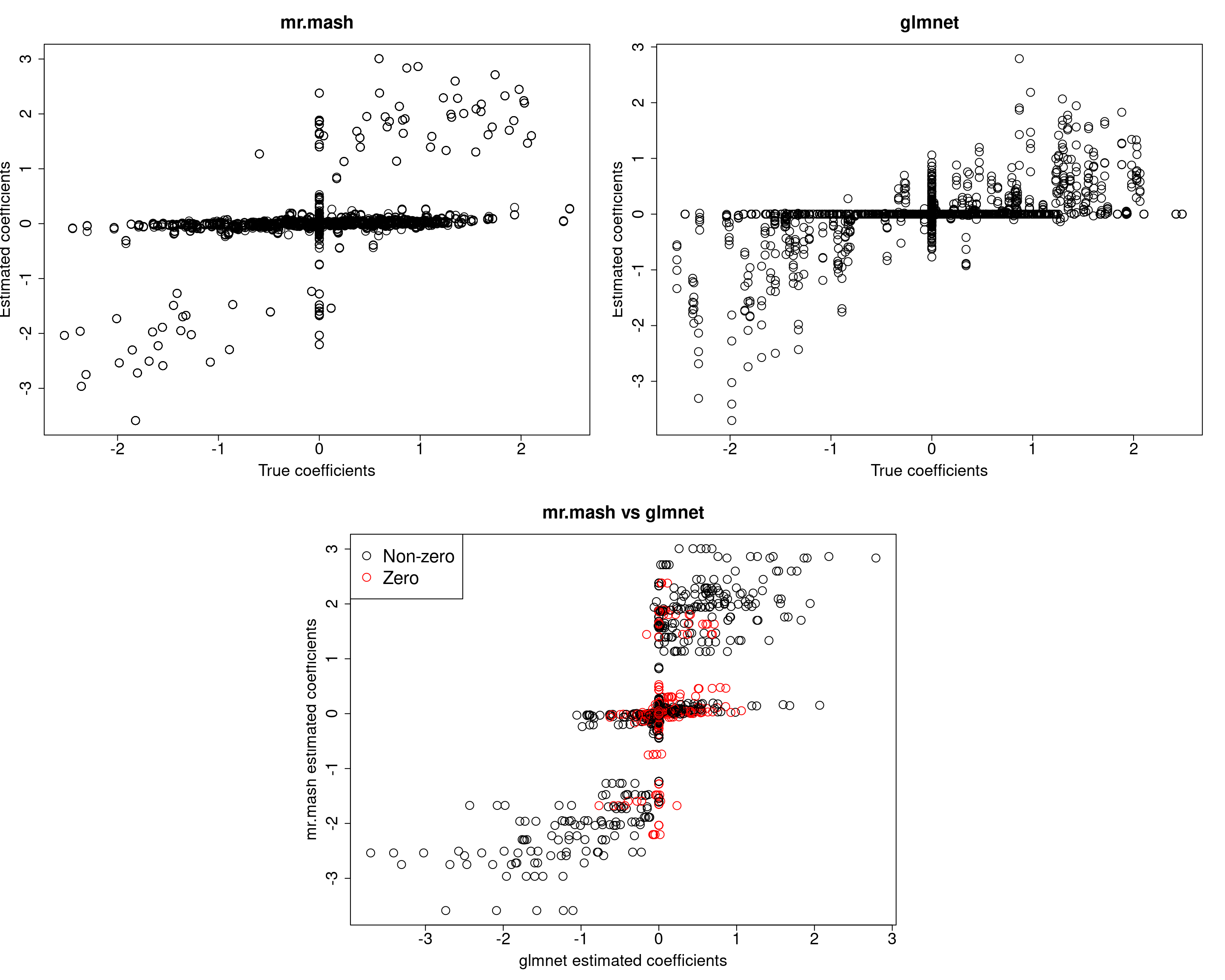
| Version | Author | Date |
|---|---|---|
| 01e3909 | fmorgante | 2020-06-03 |
print("Prediction performance with glmnet")[1] "Prediction performance with glmnet"compute_accuracy(Ytest, Yhat_test_glmnet)$bias
[1] 0.8518387 1.1181319 1.2890366 1.0579858 1.0070721
$r2
[1] 0.07926694 0.12502546 0.14366905 0.09959621 0.09842417
$mse
[1] 547.1047 567.8887 616.0232 521.4515 547.9793print("Prediction performance with mr.mash")[1] "Prediction performance with mr.mash"compute_accuracy(Ytest, Yhat_test_mrmash_fixV)$bias
[1] 0.4530571 0.5552930 0.6208323 0.4792331 0.5243710
$r2
[1] 0.09099277 0.12430902 0.14253512 0.10442110 0.11910132
$mse
[1] 617.4501 619.5676 650.5751 590.2828 595.2566Prediction performance looks worse in terms of MSE. However, looking at the plots of the coefficients, we can see that many coefficients are no longer overshrunk. Let’s see what happens if we initialize V to the truth but then we update it.
###Fit mr.mash
fit_mrmash_initV <- mr.mash(Xtrain, Ytrain, S0, tol=1e-2, convergence_criterion="ELBO", update_w0=TRUE,
                     update_w0_method="EM", compute_ELBO=TRUE, standardize=FALSE, verbose=FALSE, update_V=TRUE,
                     mu1_init = Bhat_glmnet, w0_threshold=1e-8, V=out$V)
Yhat_test_mrmash_initV <- predict(fit_mrmash_initV, Xtest)
layout(matrix(c(1, 1, 2, 2,
1, 1, 2, 2,
0, 3, 3, 0,
0, 3, 3, 0), 4, 4, byrow = TRUE))
###Plot estimated vs true coeffcients
##mr.mash
plot(out$B, fit_mrmash_initV$mu1, main="mr.mash", xlab="True coefficients", ylab="Estimated coefficients",
cex=2, cex.lab=1.8, cex.main=2, cex.axis=1.8)
##glmnet
plot(out$B, Bhat_glmnet, main="glmnet", xlab="True coefficients", ylab="Estimated coefficients",
cex=2, cex.lab=1.8, cex.main=2, cex.axis=1.8)
###Plot mr.mash vs glmnet estimated coeffcients
colorz <- matrix("black", nrow=p, ncol=r)
zeros <- apply(out$B, 2, function(x) x==0)
for(i in 1:ncol(colorz)){
colorz[zeros[, i], i] <- "red"
}
plot(Bhat_glmnet, fit_mrmash_initV$mu1, main="mr.mash vs glmnet",
xlab="glmnet estimated coefficients", ylab="mr.mash estimated coefficients",
col=colorz, cex=2, cex.lab=1.8, cex.main=2, cex.axis=1.8)
legend("topleft",
legend = c("Non-zero", "Zero"),
col = c("black", "red"),
pch = c(1, 1),
horiz = FALSE,
cex=2) 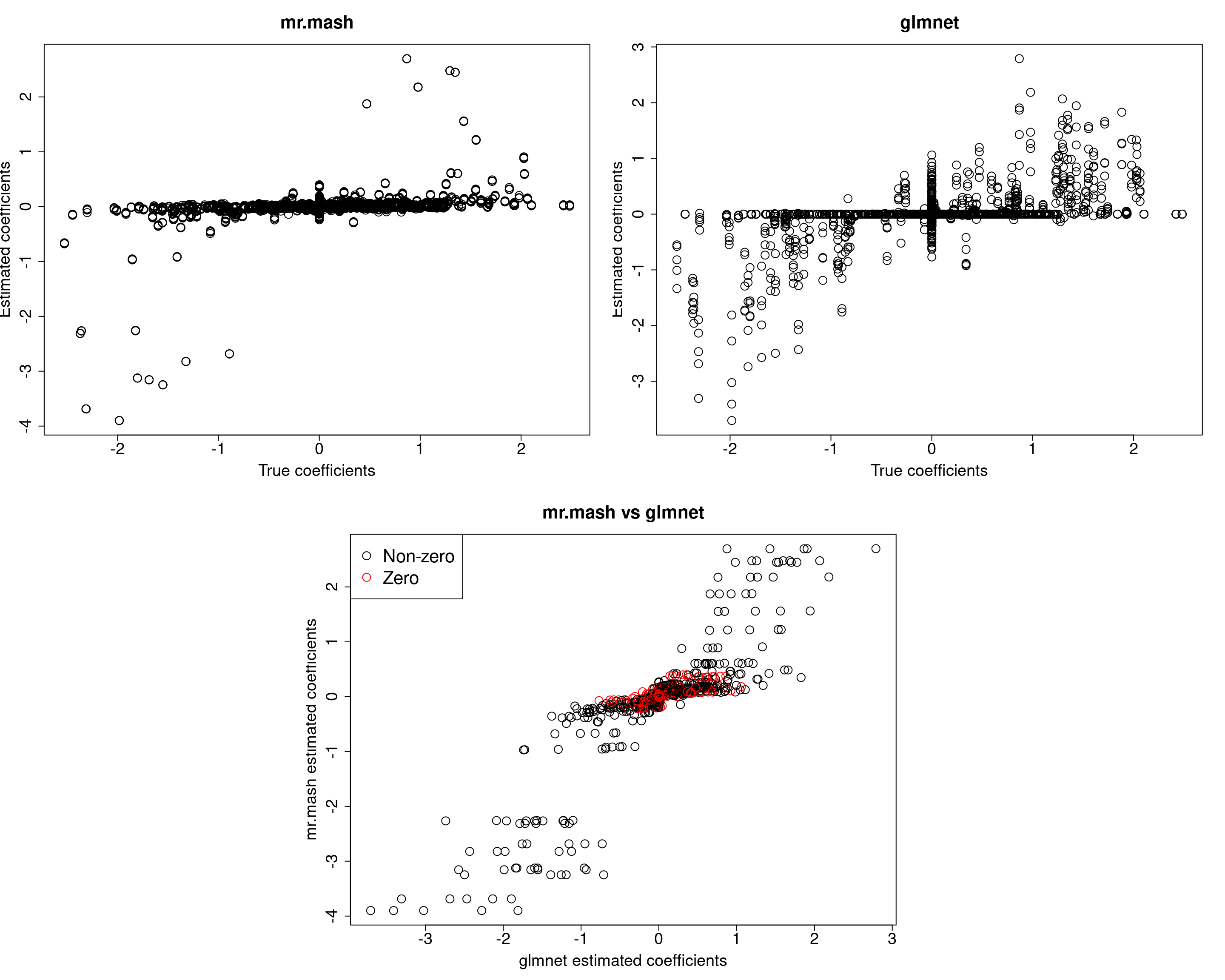
| Version | Author | Date |
|---|---|---|
| 01e3909 | fmorgante | 2020-06-03 |
print("Prediction performance with glmnet")[1] "Prediction performance with glmnet"compute_accuracy(Ytest, Yhat_test_glmnet)$bias
[1] 0.8518387 1.1181319 1.2890366 1.0579858 1.0070721
$r2
[1] 0.07926694 0.12502546 0.14366905 0.09959621 0.09842417
$mse
[1] 547.1047 567.8887 616.0232 521.4515 547.9793print("Prediction performance with mr.mash")[1] "Prediction performance with mr.mash"compute_accuracy(Ytest, Yhat_test_mrmash_initV)$bias
[1] 0.5610211 0.8151299 0.8260401 0.6687940 0.6800940
$r2
[1] 0.05632059 0.10825220 0.10223811 0.08188427 0.08061416
$mse
[1] 579.6529 581.5075 643.9059 543.2112 569.6620print("True V (full data)")[1] "True V (full data)"out$V [,1] [,2] [,3] [,4] [,5]
[1,] 318.8014 0.0000 0.0000 0.0000 0.0000
[2,] 0.0000 318.8014 0.0000 0.0000 0.0000
[3,] 0.0000 0.0000 318.8014 0.0000 0.0000
[4,] 0.0000 0.0000 0.0000 318.8014 0.0000
[5,] 0.0000 0.0000 0.0000 0.0000 318.8014print("Estimated V (training data)")[1] "Estimated V (training data)"fit_mrmash_initV$V Y1 Y2 Y3 Y4 Y5
Y1 494.4493 170.3279 163.4511 151.3242 176.9302
Y2 170.3279 532.9190 177.4565 155.0622 197.1693
Y3 163.4511 177.4565 436.2580 139.6459 186.1493
Y4 151.3242 155.0622 139.6459 382.4974 161.1707
Y5 176.9302 197.1693 186.1493 161.1707 531.1984Here, we can see that that initilizing the residual covariance to the truth leads to essentially the same solutions as using the default initialization method.
We will now update the residual covariance imposing a diagonal structure. Let’s see how that works.
###Fit mr.mash
fit_mrmash_diagV <- mr.mash(Xtrain, Ytrain, S0, tol=1e-2, convergence_criterion="ELBO", update_w0=TRUE,
                            update_w0_method="EM", compute_ELBO=TRUE, standardize=FALSE, verbose=FALSE, update_V=TRUE,
                            update_V_method="diagonal", mu1_init=Bhat_glmnet, w0_threshold=1e-8)
Yhat_test_mrmash_diagV <- predict(fit_mrmash_diagV, Xtest)
layout(matrix(c(1, 1, 2, 2,
1, 1, 2, 2,
0, 3, 3, 0,
0, 3, 3, 0), 4, 4, byrow = TRUE))
###Plot estimated vs true coeffcients
##mr.mash
plot(out$B, fit_mrmash_diagV$mu1, main="mr.mash", xlab="True coefficients", ylab="Estimated coefficients",
cex=2, cex.lab=1.8, cex.main=2, cex.axis=1.8)
##glmnet
plot(out$B, Bhat_glmnet, main="glmnet", xlab="True coefficients", ylab="Estimated coefficients",
cex=2, cex.lab=1.8, cex.main=2, cex.axis=1.8)
###Plot mr.mash vs glmnet estimated coeffcients
colorz <- matrix("black", nrow=p, ncol=r)
zeros <- apply(out$B, 2, function(x) x==0)
for(i in 1:ncol(colorz)){
colorz[zeros[, i], i] <- "red"
}
plot(Bhat_glmnet, fit_mrmash_diagV$mu1, main="mr.mash vs glmnet",
xlab="glmnet estimated coefficients", ylab="mr.mash estimated coefficients",
col=colorz, cex=2, cex.lab=1.8, cex.main=2, cex.axis=1.8)
legend("topleft",
legend = c("Non-zero", "Zero"),
col = c("black", "red"),
pch = c(1, 1),
horiz = FALSE,
cex=2) 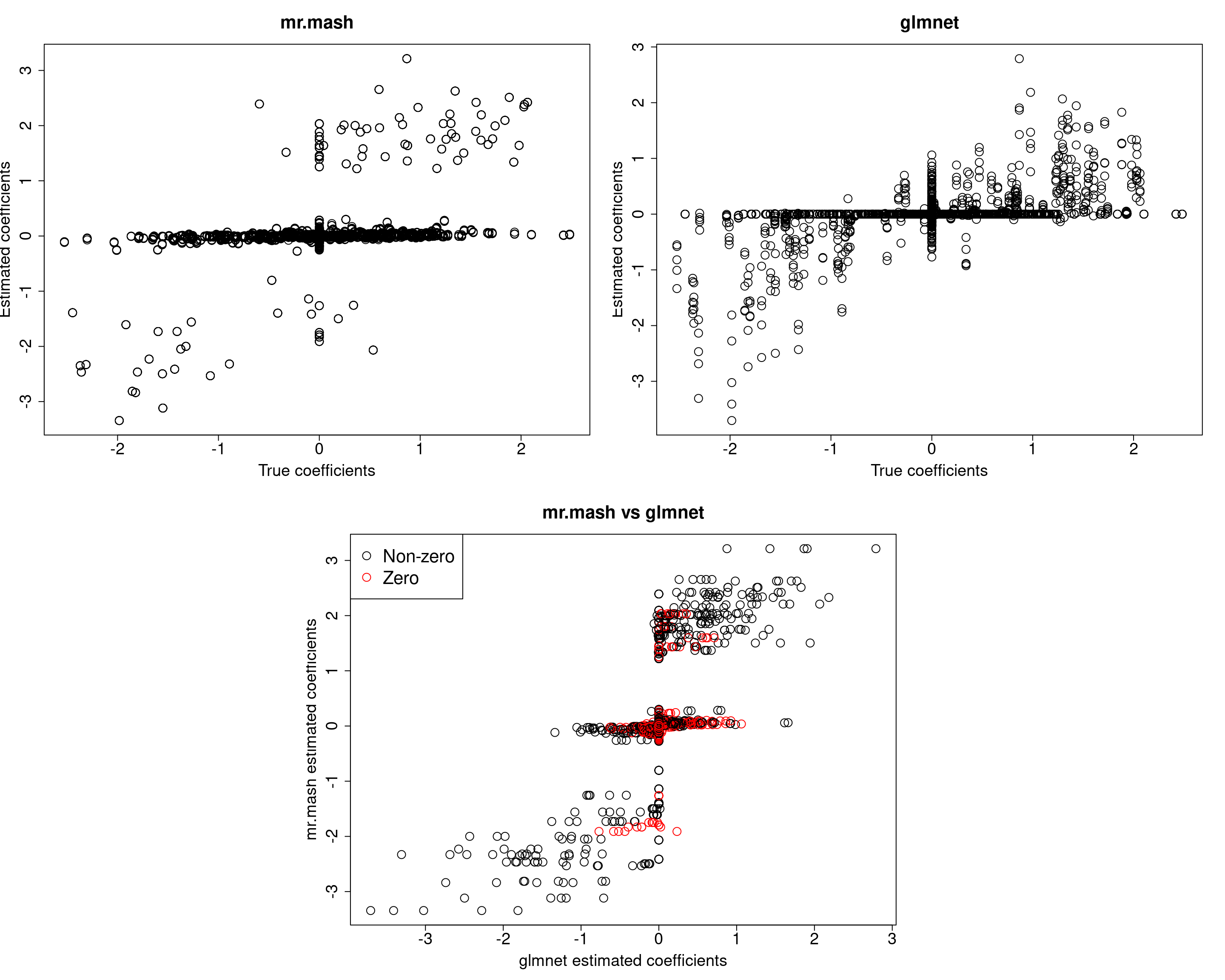
| Version | Author | Date |
|---|---|---|
| 01e3909 | fmorgante | 2020-06-03 |
print("Prediction performance with glmnet")[1] "Prediction performance with glmnet"compute_accuracy(Ytest, Yhat_test_glmnet)$bias
[1] 0.8518387 1.1181319 1.2890366 1.0579858 1.0070721
$r2
[1] 0.07926694 0.12502546 0.14366905 0.09959621 0.09842417
$mse
[1] 547.1047 567.8887 616.0232 521.4515 547.9793print("Prediction performance with mr.mash")[1] "Prediction performance with mr.mash"compute_accuracy(Ytest, Yhat_test_mrmash_diagV)$bias
[1] 0.4590680 0.5441586 0.6004030 0.4286839 0.5007622
$r2
[1] 0.09625995 0.12339177 0.13733223 0.08599529 0.11179664
$mse
[1] 614.5711 623.3936 657.9755 616.9041 607.0033print("True V (full data)")[1] "True V (full data)"out$V [,1] [,2] [,3] [,4] [,5]
[1,] 318.8014 0.0000 0.0000 0.0000 0.0000
[2,] 0.0000 318.8014 0.0000 0.0000 0.0000
[3,] 0.0000 0.0000 318.8014 0.0000 0.0000
[4,] 0.0000 0.0000 0.0000 318.8014 0.0000
[5,] 0.0000 0.0000 0.0000 0.0000 318.8014print("Estimated V (training data)")[1] "Estimated V (training data)"fit_mrmash_diagV$V Y1 Y2 Y3 Y4 Y5
Y1 325.9281 0.0000 0.0000 0.0000 0.0000
Y2 0.0000 379.5774 0.0000 0.0000 0.0000
Y3 0.0000 0.0000 299.4771 0.0000 0.0000
Y4 0.0000 0.0000 0.0000 268.2436 0.0000
Y5 0.0000 0.0000 0.0000 0.0000 380.3463Although the estimated residual covariance is much closer to the truth and now many coefficients are not overshrunk, prediction performance is still poor. Another possibility is that overshrinking of coefficients happens because the mixture weights are poorly initialized. Let’s now try to initialize the mixture weights to the truth.
###Fit mr.mash
w0init <- rep(0, length(S0))
w0init[c(143, 151)] <- c(0.5, 0.5)
fit_mrmash_diagV_initw0 <- mr.mash(Xtrain, Ytrain, S0, w0=w0init, tol=1e-2, convergence_criterion="ELBO", update_w0=TRUE,
                                   update_w0_method="EM", compute_ELBO=TRUE, standardize=FALSE, verbose=FALSE, update_V=TRUE,
                                   update_V_method="diagonal", mu1_init=Bhat_glmnet, w0_threshold=0)
Yhat_test_mrmash_diagV_initw0 <- predict(fit_mrmash_diagV_initw0, Xtest)
layout(matrix(c(1, 1, 2, 2,
1, 1, 2, 2,
0, 3, 3, 0,
0, 3, 3, 0), 4, 4, byrow = TRUE))
###Plot estimated vs true coeffcients
##mr.mash
plot(out$B, fit_mrmash_diagV_initw0$mu1, main="mr.mash", xlab="True coefficients", ylab="Estimated coefficients",
cex=2, cex.lab=1.8, cex.main=2, cex.axis=1.8)
##glmnet
plot(out$B, Bhat_glmnet, main="glmnet", xlab="True coefficients", ylab="Estimated coefficients",
cex=2, cex.lab=1.8, cex.main=2, cex.axis=1.8)
###Plot mr.mash vs glmnet estimated coeffcients
colorz <- matrix("black", nrow=p, ncol=r)
zeros <- apply(out$B, 2, function(x) x==0)
for(i in 1:ncol(colorz)){
colorz[zeros[, i], i] <- "red"
}
plot(Bhat_glmnet, fit_mrmash_diagV_initw0$mu1, main="mr.mash vs glmnet",
xlab="glmnet estimated coefficients", ylab="mr.mash estimated coefficients",
col=colorz, cex=2, cex.lab=1.8, cex.main=2, cex.axis=1.8)
legend("topleft",
legend = c("Non-zero", "Zero"),
col = c("black", "red"),
pch = c(1, 1),
horiz = FALSE,
cex=2) 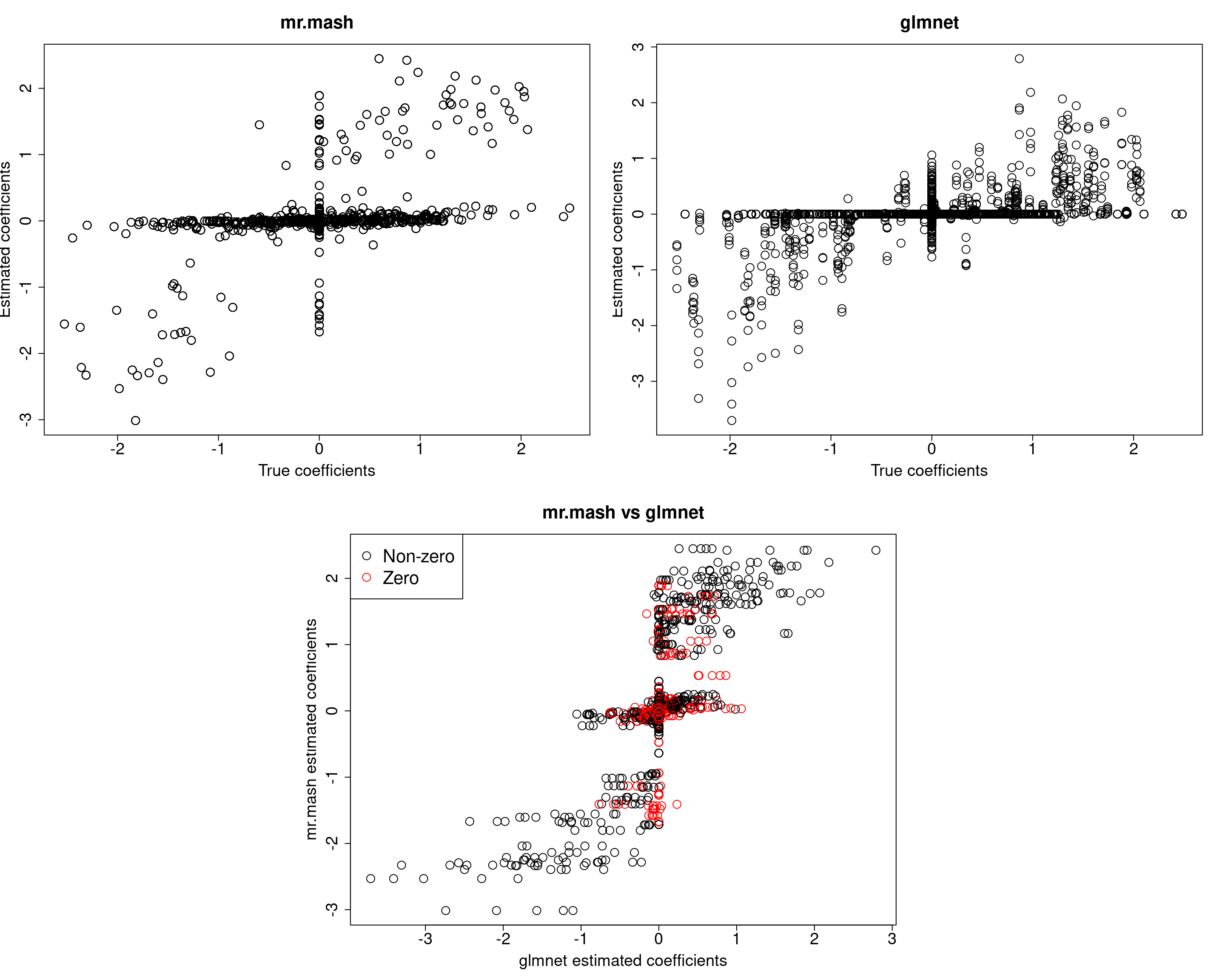
| Version | Author | Date |
|---|---|---|
| 01e3909 | fmorgante | 2020-06-03 |
print("Prediction performance with glmnet")[1] "Prediction performance with glmnet"compute_accuracy(Ytest, Yhat_test_glmnet)$bias
[1] 0.8518387 1.1181319 1.2890366 1.0579858 1.0070721
$r2
[1] 0.07926694 0.12502546 0.14366905 0.09959621 0.09842417
$mse
[1] 547.1047 567.8887 616.0232 521.4515 547.9793print("Prediction performance with mr.mash")[1] "Prediction performance with mr.mash"compute_accuracy(Ytest, Yhat_test_mrmash_diagV_initw0)$bias
[1] 0.5650397 0.7052100 0.7861362 0.6137133 0.6712195
$r2
[1] 0.1009943 0.1441554 0.1629976 0.1221435 0.1390226
$mse
[1] 568.1387 570.7545 605.8555 536.1243 543.4498print("True V (full data)")[1] "True V (full data)"out$V [,1] [,2] [,3] [,4] [,5]
[1,] 318.8014 0.0000 0.0000 0.0000 0.0000
[2,] 0.0000 318.8014 0.0000 0.0000 0.0000
[3,] 0.0000 0.0000 318.8014 0.0000 0.0000
[4,] 0.0000 0.0000 0.0000 318.8014 0.0000
[5,] 0.0000 0.0000 0.0000 0.0000 318.8014print("Estimated V (training data)")[1] "Estimated V (training data)"fit_mrmash_diagV_initw0$V Y1 Y2 Y3 Y4 Y5
Y1 342.8592 0.0000 0.0000 0.0000 0.0000
Y2 0.0000 395.7401 0.0000 0.0000 0.0000
Y3 0.0000 0.0000 311.0833 0.0000 0.0000
Y4 0.0000 0.0000 0.0000 271.6935 0.0000
Y5 0.0000 0.0000 0.0000 0.0000 379.1278Now, prediction performance is better. Next, let’s try to fix the mixture weights to the truth.
###Fit mr.mash
closest_comp <- grid[which.min(abs(0.9-grid))]
S0fix <- list(S0_1=matrix(closest_comp, r, r), S0_2=matrix(0, r, r))
w0fix <- c(0.5, 0.5)

fit_mrmash_diagV_truew0 <- mr.mash(Xtrain, Ytrain, S0fix, w0=w0fix, tol=1e-2, convergence_criterion="ELBO", update_w0=FALSE,
                                    update_w0_method="EM", compute_ELBO=TRUE, standardize=FALSE, verbose=FALSE, update_V=TRUE,
                                    update_V_method="diagonal", mu1_init=Bhat_glmnet, w0_threshold=1e-8)
Yhat_test_mrmash_diagV_truew0 <- predict(fit_mrmash_diagV_truew0, Xtest)
layout(matrix(c(1, 1, 2, 2,
1, 1, 2, 2,
0, 3, 3, 0,
0, 3, 3, 0), 4, 4, byrow = TRUE))
###Plot estimated vs true coeffcients
##mr.mash
plot(out$B, fit_mrmash_diagV_truew0$mu1, main="mr.mash", xlab="True coefficients", ylab="Estimated coefficients",
cex=2, cex.lab=1.8, cex.main=2, cex.axis=1.8)
##glmnet
plot(out$B, Bhat_glmnet, main="glmnet", xlab="True coefficients", ylab="Estimated coefficients",
cex=2, cex.lab=1.8, cex.main=2, cex.axis=1.8)
###Plot mr.mash vs glmnet estimated coeffcients
colorz <- matrix("black", nrow=p, ncol=r)
zeros <- apply(out$B, 2, function(x) x==0)
for(i in 1:ncol(colorz)){
colorz[zeros[, i], i] <- "red"
}
plot(Bhat_glmnet, fit_mrmash_diagV_truew0$mu1, main="mr.mash vs glmnet",
xlab="glmnet estimated coefficients", ylab="mr.mash estimated coefficients",
col=colorz, cex=2, cex.lab=1.8, cex.main=2, cex.axis=1.8)
legend("topleft",
legend = c("Non-zero", "Zero"),
col = c("black", "red"),
pch = c(1, 1),
horiz = FALSE,
cex=2) 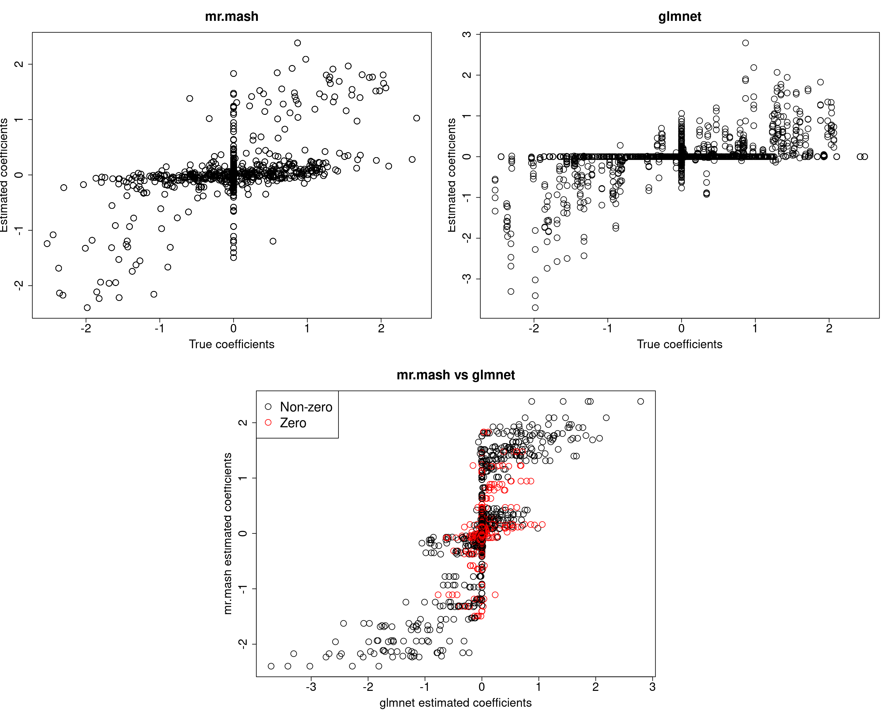
| Version | Author | Date |
|---|---|---|
| 01e3909 | fmorgante | 2020-06-03 |
print("Prediction performance with glmnet")[1] "Prediction performance with glmnet"compute_accuracy(Ytest, Yhat_test_glmnet)$bias
[1] 0.8518387 1.1181319 1.2890366 1.0579858 1.0070721
$r2
[1] 0.07926694 0.12502546 0.14366905 0.09959621 0.09842417
$mse
[1] 547.1047 567.8887 616.0232 521.4515 547.9793print("Prediction performance with mr.mash")[1] "Prediction performance with mr.mash"compute_accuracy(Ytest, Yhat_test_mrmash_diagV_truew0)$bias
[1] 0.7106733 0.8601239 0.9169594 0.7243430 0.7988996
$r2
[1] 0.1434966 0.1926099 0.1991813 0.1528236 0.1768900
$mse
[1] 521.4989 525.9623 572.0003 502.8177 506.7851print("True V (full data)")[1] "True V (full data)"out$V [,1] [,2] [,3] [,4] [,5]
[1,] 318.8014 0.0000 0.0000 0.0000 0.0000
[2,] 0.0000 318.8014 0.0000 0.0000 0.0000
[3,] 0.0000 0.0000 318.8014 0.0000 0.0000
[4,] 0.0000 0.0000 0.0000 318.8014 0.0000
[5,] 0.0000 0.0000 0.0000 0.0000 318.8014print("Estimated V (training data)")[1] "Estimated V (training data)"fit_mrmash_diagV_truew0$V Y1 Y2 Y3 Y4 Y5
Y1 349.3808 0.0000 0.0000 0.0000 0.0000
Y2 0.0000 396.0128 0.0000 0.0000 0.0000
Y3 0.0000 0.0000 311.7625 0.0000 0.0000
Y4 0.0000 0.0000 0.0000 278.3492 0.0000
Y5 0.0000 0.0000 0.0000 0.0000 380.7376Prediction accuracy is now good and better than group-lasso. Finally, let’s fix both the residual covariance and mixture weights to the truth.
###Fit mr.mash
fit_mrmash_trueV_truew0 <- mr.mash(Xtrain, Ytrain, S0fix, w0=w0fix, tol=1e-2, convergence_criterion="ELBO", update_w0=FALSE,
                                    update_w0_method="EM", compute_ELBO=TRUE, standardize=FALSE, verbose=FALSE, update_V=FALSE,
                                    update_V_method="diagonal", mu1_init=Bhat_glmnet, w0_threshold=1e-8, V=out$V)
Yhat_test_mrmash_trueV_truew0 <- predict(fit_mrmash_trueV_truew0, Xtest)
layout(matrix(c(1, 1, 2, 2,
1, 1, 2, 2,
0, 3, 3, 0,
0, 3, 3, 0), 4, 4, byrow = TRUE))
###Plot estimated vs true coeffcients
##mr.mash
plot(out$B, fit_mrmash_trueV_truew0$mu1, main="mr.mash", xlab="True coefficients", ylab="Estimated coefficients",
cex=2, cex.lab=1.8, cex.main=2, cex.axis=1.8)
##glmnet
plot(out$B, Bhat_glmnet, main="glmnet", xlab="True coefficients", ylab="Estimated coefficients",
cex=2, cex.lab=1.8, cex.main=2, cex.axis=1.8)
###Plot mr.mash vs glmnet estimated coeffcients
colorz <- matrix("black", nrow=p, ncol=r)
zeros <- apply(out$B, 2, function(x) x==0)
for(i in 1:ncol(colorz)){
colorz[zeros[, i], i] <- "red"
}
plot(Bhat_glmnet, fit_mrmash_trueV_truew0$mu1, main="mr.mash vs glmnet",
xlab="glmnet estimated coefficients", ylab="mr.mash estimated coefficients",
col=colorz, cex=2, cex.lab=1.8, cex.main=2, cex.axis=1.8)
legend("topleft",
legend = c("Non-zero", "Zero"),
col = c("black", "red"),
pch = c(1, 1),
horiz = FALSE,
cex=2) 
| Version | Author | Date |
|---|---|---|
| 01e3909 | fmorgante | 2020-06-03 |
print("Prediction performance with glmnet")[1] "Prediction performance with glmnet"compute_accuracy(Ytest, Yhat_test_glmnet)$bias
[1] 0.8518387 1.1181319 1.2890366 1.0579858 1.0070721
$r2
[1] 0.07926694 0.12502546 0.14366905 0.09959621 0.09842417
$mse
[1] 547.1047 567.8887 616.0232 521.4515 547.9793print("Prediction performance with mr.mash")[1] "Prediction performance with mr.mash"compute_accuracy(Ytest, Yhat_test_mrmash_trueV_truew0)$bias
[1] 0.7034135 0.8297291 0.8671787 0.6870042 0.7695739
$r2
[1] 0.1560834 0.1990046 0.1977877 0.1526351 0.1822440
$mse
[1] 516.4040 524.0623 575.3026 508.5362 506.6930Not surprisingly, we now achieve the best accuracy of all models.
However, looking at ELBO for all the models fitted so far reveals something interesting. The models that provide the best prediction performance in the test set are those with smaller ELBO, and viceversa. My intuition is that the largest ELBO is due to those models having more free parameters (since they include updating the weights and V with no structure imposed).
print(paste("Update w0, update V:", fit_mrmash$ELBO))[1] "Update w0, update V: -11175.3962254482"print(paste("Update w0, fix V to the truth:", fit_mrmash_fixV$ELBO))[1] "Update w0, fix V to the truth: -11239.6904501032"print(paste("Update w0, update V initializing it to the truth:", fit_mrmash_initV$ELBO))[1] "Update w0, update V initializing it to the truth: -11175.3937438927"print(paste("Update w0, update V imposing a diagonal structure:", fit_mrmash_diagV$ELBO))[1] "Update w0, update V imposing a diagonal structure: -11227.0476540694"print(paste("Update w0 initializing them to the truth, update V imposing a diagonal structure:", fit_mrmash_diagV_initw0$ELBO))[1] "Update w0 initializing them to the truth, update V imposing a diagonal structure: -11241.8971374156"print(paste("Fix w0 to the truth, update V imposing a diagonal structure:", fit_mrmash_diagV_truew0$ELBO))[1] "Fix w0 to the truth, update V imposing a diagonal structure: -11319.1170084933"print(paste("Fix w0 and V to the truth:", fit_mrmash_trueV_truew0$ELBO))[1] "Fix w0 and V to the truth: -11328.5451731686"Sparser scenario
For comparison let’s try to repeat the analysis above (updating V) on a sparser scenario, i.e., p_causal=50.
###Set parameters
n <- 1000
p <- 1000
p_causal <- 50
r <- 5
r_causal <- r
pve <- 0.5
B_cor <- 1
X_cor <- 0
V_cor <- 0

###Simulate V, B, X and Y
out50 <- mr.mash.alpha:::simulate_mr_mash_data(n, p, p_causal, r, r_causal=r, intercepts = rep(1, r),
                                             pve=pve, B_cor=B_cor, B_scale=0.9, X_cor=X_cor, X_scale=0.8, V_cor=V_cor)

colnames(out50$Y) <- paste0("Y", seq(1, r))
rownames(out50$Y) <- paste0("N", seq(1, n))
colnames(out50$X) <- paste0("X", seq(1, p))
rownames(out50$X) <- paste0("N", seq(1, n))

###Split the data in training and test sets
test_set50 <- sort(sample(x=c(1:n), size=round(n*0.5), replace=FALSE))
Ytrain50 <- out50$Y[-test_set50, ]
Xtrain50 <- out50$X[-test_set50, ]
Ytest50 <- out50$Y[test_set50, ]
Xtest50 <- out50$X[test_set50, ]

###Fit group-lasso
cvfit_glmnet50 <- cv.glmnet(x=Xtrain50, y=Ytrain50, family="mgaussian", alpha=1, standardize=FALSE)
coeff_glmnet50 <- coef(cvfit_glmnet50, s="lambda.min")
Bhat_glmnet50 <- matrix(as.numeric(NA), nrow=p, ncol=r)
ahat_glmnet50 <- vector("numeric", r)
for(i in 1:length(coeff_glmnet50)){
  Bhat_glmnet50[, i] <- as.vector(coeff_glmnet50[[i]])[-1]
  ahat_glmnet50[i] <- as.vector(coeff_glmnet50[[i]])[1]
}
Yhat_test_glmnet50 <- drop(predict(cvfit_glmnet50, newx=Xtest50, s="lambda.min"))

###Fit mr.mash
fit_mrmash50 <- mr.mash(Xtrain50, Ytrain50, S0, tol=1e-2, convergence_criterion="ELBO", update_w0=TRUE,
                     update_w0_method="EM", compute_ELBO=TRUE, standardize=FALSE, verbose=FALSE, update_V=TRUE,
                     mu1_init = Bhat_glmnet50, w0_threshold=1e-8)
Yhat_test_mrmash50 <- predict(fit_mrmash50, Xtest50)
layout(matrix(c(1, 1, 2, 2,
1, 1, 2, 2,
0, 3, 3, 0,
0, 3, 3, 0), 4, 4, byrow = TRUE))
###Plot estimated vs true coeffcients
##mr.mash
plot(out50$B, fit_mrmash50$mu1, main="mr.mash", xlab="True coefficients", ylab="Estimated coefficients",
cex=2, cex.lab=1.8, cex.main=2, cex.axis=1.8)
##glmnet
plot(out50$B, Bhat_glmnet50, main="glmnet", xlab="True coefficients", ylab="Estimated coefficients",
cex=2, cex.lab=1.8, cex.main=2, cex.axis=1.8)
###Plot mr.mash vs glmnet estimated coeffcients
colorz <- matrix("black", nrow=p, ncol=r)
zeros <- apply(out50$B, 2, function(x) x==0)
for(i in 1:ncol(colorz)){
colorz[zeros[, i], i] <- "red"
}
plot(Bhat_glmnet50, fit_mrmash50$mu1, main="mr.mash vs glmnet",
xlab="glmnet estimated coefficients", ylab="mr.mash estimated coefficients",
col=colorz, cex=2, cex.lab=1.8, cex.main=2, cex.axis=1.8)
legend("topleft",
legend = c("Non-zero", "Zero"),
col = c("black", "red"),
pch = c(1, 1),
horiz = FALSE,
cex=2) 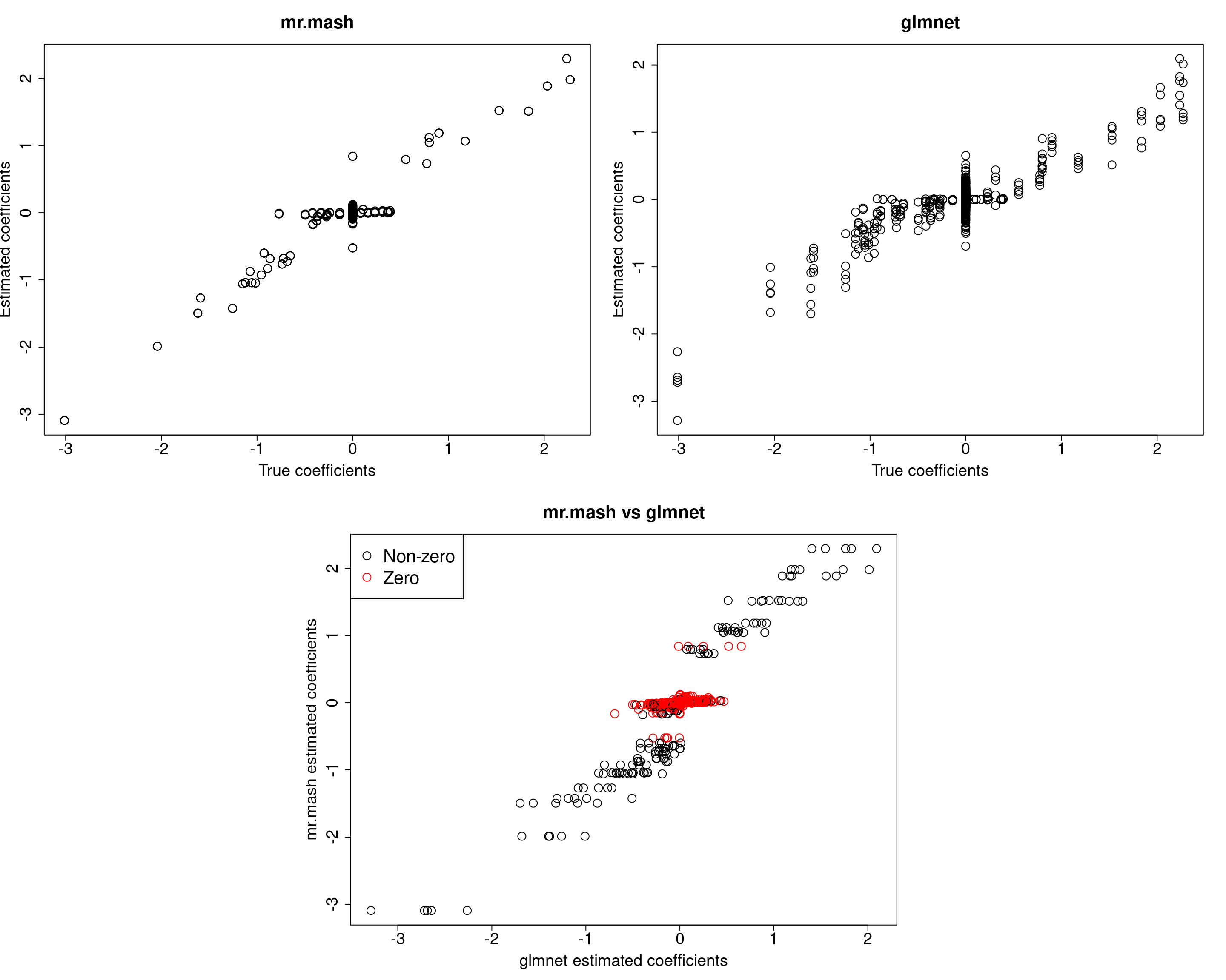
| Version | Author | Date |
|---|---|---|
| 01e3909 | fmorgante | 2020-06-03 |
print("Prediction performance with glmnet")[1] "Prediction performance with glmnet"compute_accuracy(Ytest50, Yhat_test_glmnet50)$bias
[1] 1.195819 1.379157 1.080143 1.294941 1.253665
$r2
[1] 0.4146822 0.4619715 0.3858639 0.4600377 0.3897421
$mse
[1] 55.76038 59.28675 57.89934 54.82581 64.95119print("Prediction performance with mr.mash")[1] "Prediction performance with mr.mash"compute_accuracy(Ytest50, Yhat_test_mrmash50)$bias
[1] 0.9605322 1.0451756 0.9323631 1.0078177 0.9970912
$r2
[1] 0.4932532 0.5287686 0.4657318 0.5208618 0.4758840
$mse
[1] 47.46795 48.93416 50.37683 46.62724 54.46268print("True V (full data)")[1] "True V (full data)"out50$V [,1] [,2] [,3] [,4] [,5]
[1,] 48.70994 0.00000 0.00000 0.00000 0.00000
[2,] 0.00000 48.70994 0.00000 0.00000 0.00000
[3,] 0.00000 0.00000 48.70994 0.00000 0.00000
[4,] 0.00000 0.00000 0.00000 48.70994 0.00000
[5,] 0.00000 0.00000 0.00000 0.00000 48.70994print("Estimated V (training data)")[1] "Estimated V (training data)"fit_mrmash50$V Y1 Y2 Y3 Y4 Y5
Y1 45.96214410 3.696660 2.0791487 0.6975673 0.04477361
Y2 3.69666023 47.333638 -2.1948288 2.9340544 1.45354533
Y3 2.07914867 -2.194829 48.2164300 4.4873530 -0.66300263
Y4 0.69756732 2.934054 4.4873530 53.0158990 -0.72472854
Y5 0.04477361 1.453545 -0.6630026 -0.7247285 50.22435028The results of this simulation look very good in terms of prediction performance, estimation of the coefficients, and estimation of the residual covariance.
Dense scenario (fewer variables)
Just as an additional test let’s now try to maintain the same signal-to-noise ratio as the first simulation but with fewer total variables, i.e., p=500 and p_causal=250.
###Set parameters
n <- 1000
p <- 500
p_causal <- 250
r <- 5
r_causal <- r
pve <- 0.5
B_cor <- 1
X_cor <- 0
V_cor <- 0

###Simulate V, B, X and Y
out500 <- mr.mash.alpha:::simulate_mr_mash_data(n, p, p_causal, r, r_causal=r, intercepts = rep(1, r),
                                             pve=pve, B_cor=B_cor, B_scale=0.9, X_cor=X_cor, X_scale=0.8, V_cor=V_cor)

colnames(out500$Y) <- paste0("Y", seq(1, r))
rownames(out500$Y) <- paste0("N", seq(1, n))
colnames(out500$X) <- paste0("X", seq(1, p))
rownames(out500$X) <- paste0("N", seq(1, n))

###Split the data in training and test sets
test_set500 <- sort(sample(x=c(1:n), size=round(n*0.5), replace=FALSE))
Ytrain500 <- out500$Y[-test_set500, ]
Xtrain500 <- out500$X[-test_set500, ]
Ytest500 <- out500$Y[test_set500, ]
Xtest500 <- out500$X[test_set500, ]

###Fit group-lasso
cvfit_glmnet500 <- cv.glmnet(x=Xtrain500, y=Ytrain500, family="mgaussian", alpha=1, standardize=FALSE)
coeff_glmnet500 <- coef(cvfit_glmnet500, s="lambda.min")
Bhat_glmnet500 <- matrix(as.numeric(NA), nrow=p, ncol=r)
ahat_glmnet500 <- vector("numeric", r)
for(i in 1:length(coeff_glmnet500)){
  Bhat_glmnet500[, i] <- as.vector(coeff_glmnet500[[i]])[-1]
  ahat_glmnet500[i] <- as.vector(coeff_glmnet500[[i]])[1]
}
Yhat_test_glmnet500 <- drop(predict(cvfit_glmnet500, newx=Xtest500, s="lambda.min"))

###Fit mr.mash
fit_mrmash500 <- mr.mash(Xtrain500, Ytrain500, S0, tol=1e-2, convergence_criterion="ELBO", update_w0=TRUE,
                     update_w0_method="EM", compute_ELBO=TRUE, standardize=FALSE, verbose=FALSE, update_V=TRUE,
                     mu1_init = Bhat_glmnet500, w0_threshold=1e-8)
Yhat_test_mrmash500 <- predict(fit_mrmash500, Xtest500)
layout(matrix(c(1, 1, 2, 2,
1, 1, 2, 2,
0, 3, 3, 0,
0, 3, 3, 0), 4, 4, byrow = TRUE))
###Plot estimated vs true coeffcients
##mr.mash
plot(out500$B, fit_mrmash500$mu1, main="mr.mash", xlab="True coefficients", ylab="Estimated coefficients",
cex=2, cex.lab=1.8, cex.main=2, cex.axis=1.8)
##glmnet
plot(out500$B, Bhat_glmnet500, main="glmnet", xlab="True coefficients", ylab="Estimated coefficients",
cex=2, cex.lab=1.8, cex.main=2, cex.axis=1.8)
###Plot mr.mash vs glmnet estimated coeffcients
colorz <- matrix("black", nrow=p, ncol=r)
zeros <- apply(out500$B, 2, function(x) x==0)
for(i in 1:ncol(colorz)){
colorz[zeros[, i], i] <- "red"
}
plot(Bhat_glmnet500, fit_mrmash500$mu1, main="mr.mash vs glmnet",
xlab="glmnet estimated coefficients", ylab="mr.mash estimated coefficients",
col=colorz, cex=2, cex.lab=1.8, cex.main=2, cex.axis=1.8)
legend("topleft",
legend = c("Non-zero", "Zero"),
col = c("black", "red"),
pch = c(1, 1),
horiz = FALSE,
cex=2) 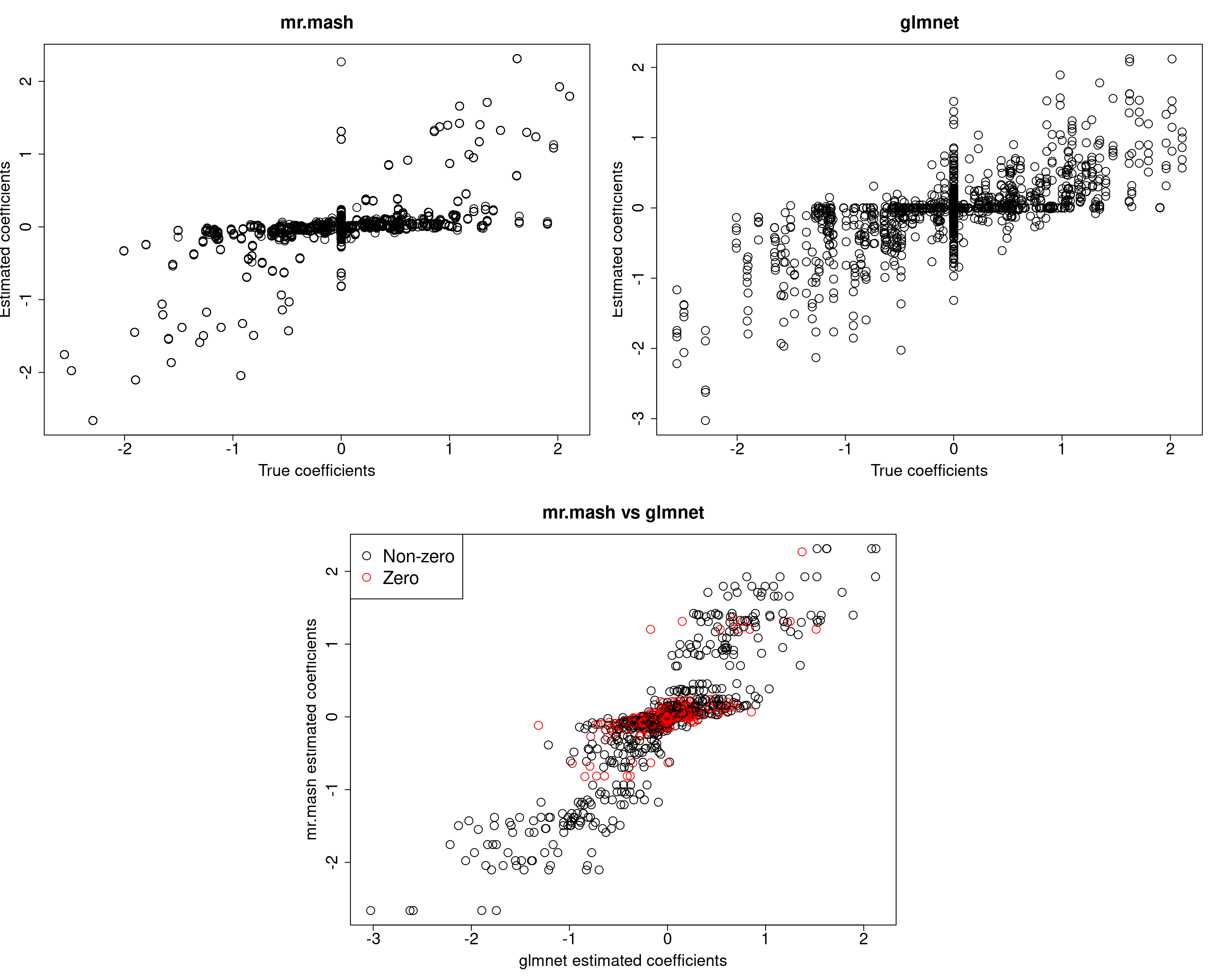
| Version | Author | Date |
|---|---|---|
| 01e3909 | fmorgante | 2020-06-03 |
print("Prediction performance with glmnet")[1] "Prediction performance with glmnet"compute_accuracy(Ytest500, Yhat_test_glmnet500)$bias
[1] 1.1135057 1.1448266 1.1831552 1.1210518 0.9469529
$r2
[1] 0.2472891 0.2115488 0.2502438 0.2205002 0.2275750
$mse
[1] 242.8296 244.6767 248.4512 241.5001 212.1975print("Prediction performance with mr.mash")[1] "Prediction performance with mr.mash"compute_accuracy(Ytest500, Yhat_test_mrmash500)$bias
[1] 0.9457993 0.9275316 1.0052297 0.9303536 0.8669876
$r2
[1] 0.2426038 0.2472925 0.2671149 0.2420950 0.2529487
$mse
[1] 242.3914 231.7617 240.9589 234.4983 206.0967print("True V (full data)")[1] "True V (full data)"out500$V [,1] [,2] [,3] [,4] [,5]
[1,] 158.7435 0.0000 0.0000 0.0000 0.0000
[2,] 0.0000 158.7435 0.0000 0.0000 0.0000
[3,] 0.0000 0.0000 158.7435 0.0000 0.0000
[4,] 0.0000 0.0000 0.0000 158.7435 0.0000
[5,] 0.0000 0.0000 0.0000 0.0000 158.7435print("Estimated V (training data)")[1] "Estimated V (training data)"fit_mrmash500$V Y1 Y2 Y3 Y4 Y5
Y1 183.04474 32.637629 28.99554 29.034766 34.112325
Y2 32.63763 180.053159 32.29493 5.908755 7.772015
Y3 28.99554 32.294929 197.99964 26.728751 27.351392
Y4 29.03477 5.908755 26.72875 180.464744 27.574611
Y5 34.11233 7.772015 27.35139 27.574611 169.668844In this last simulation, we can see that mr.mash performs pretty well, even in a denser scenario with fewer variables.
sessionInfo()R version 3.5.1 (2018-07-02)
Platform: x86_64-pc-linux-gnu (64-bit)
Running under: Scientific Linux 7.4 (Nitrogen)
Matrix products: default
BLAS/LAPACK: /software/openblas-0.2.19-el7-x86_64/lib/libopenblas_haswellp-r0.2.19.so
locale:
[1] LC_CTYPE=en_US.UTF-8 LC_NUMERIC=C
[3] LC_TIME=en_US.UTF-8 LC_COLLATE=en_US.UTF-8
[5] LC_MONETARY=en_US.UTF-8 LC_MESSAGES=en_US.UTF-8
[7] LC_PAPER=en_US.UTF-8 LC_NAME=C
[9] LC_ADDRESS=C LC_TELEPHONE=C
[11] LC_MEASUREMENT=en_US.UTF-8 LC_IDENTIFICATION=C
attached base packages:
[1] stats graphics grDevices utils datasets methods base
other attached packages:
[1] glmnet_2.0-16 foreach_1.4.4 Matrix_1.2-15
[4] mr.mash.alpha_0.1-81
loaded via a namespace (and not attached):
[1] MBSP_1.0 Rcpp_1.0.4.6 compiler_3.5.1
[4] later_0.7.5 git2r_0.26.1 workflowr_1.6.2
[7] iterators_1.0.10 tools_3.5.1 digest_0.6.25
[10] evaluate_0.12 lattice_0.20-38 GIGrvg_0.5
[13] yaml_2.2.1 SparseM_1.77 mvtnorm_1.1-1
[16] coda_0.19-3 stringr_1.4.0 knitr_1.20
[19] fs_1.3.1 MatrixModels_0.4-1 rprojroot_1.3-2
[22] grid_3.5.1 glue_1.4.0 R6_2.4.1
[25] rmarkdown_1.10 mixsqp_0.3-43 irlba_2.3.3
[28] magrittr_1.5 whisker_0.3-2 codetools_0.2-15
[31] backports_1.1.5 promises_1.0.1 htmltools_0.3.6
[34] matrixStats_0.56.0 mcmc_0.9-6 MASS_7.3-51.1
[37] httpuv_1.4.5 quantreg_5.36 stringi_1.4.3
[40] MCMCpack_1.4-4