Prediction accuracy
Fabio Morgante
April 16, 2020
Last updated: 2020-04-16
Checks: 7 0
Knit directory: mr_mash_test/
This reproducible R Markdown analysis was created with workflowr (version 1.6.1). The Checks tab describes the reproducibility checks that were applied when the results were created. The Past versions tab lists the development history.
Great! Since the R Markdown file has been committed to the Git repository, you know the exact version of the code that produced these results.
Great job! The global environment was empty. Objects defined in the global environment can affect the analysis in your R Markdown file in unknown ways. For reproduciblity it’s best to always run the code in an empty environment.
The command set.seed(20200328) was run prior to running the code in the R Markdown file. Setting a seed ensures that any results that rely on randomness, e.g. subsampling or permutations, are reproducible.
Great job! Recording the operating system, R version, and package versions is critical for reproducibility.
Nice! There were no cached chunks for this analysis, so you can be confident that you successfully produced the results during this run.
Great job! Using relative paths to the files within your workflowr project makes it easier to run your code on other machines.
Great! You are using Git for version control. Tracking code development and connecting the code version to the results is critical for reproducibility.
The results in this page were generated with repository version 2e37a1d. See the Past versions tab to see a history of the changes made to the R Markdown and HTML files.
Note that you need to be careful to ensure that all relevant files for the analysis have been committed to Git prior to generating the results (you can use wflow_publish or wflow_git_commit). workflowr only checks the R Markdown file, but you know if there are other scripts or data files that it depends on. Below is the status of the Git repository when the results were generated:
Ignored files:
    Ignored:    .sos/
    Ignored:    code/fit_mr_mash.66662433.err
    Ignored:    code/fit_mr_mash.66662433.out
    Ignored:    dsc/.sos/
    Ignored:    dsc/outfiles/
    Ignored:    output/dsc.html
    Ignored:    output/dsc/

Untracked files:
    Untracked:  code/plot_test.R

Unstaged changes:
    Modified:   dsc/midway2.yml
Note that any generated files, e.g. HTML, png, CSS, etc., are not included in this status report because it is ok for generated content to have uncommitted changes.
These are the previous versions of the repository in which changes were made to the R Markdown (analysis/results_accuracy.Rmd) and HTML (docs/results_accuracy.html) files. If you’ve configured a remote Git repository (see ?wflow_git_remote), click on the hyperlinks in the table below to view the files as they were in that past version.
| File | Version | Author | Date | Message |
|---|---|---|---|---|
| html | 161eea7 | fmorgante | 2020-04-16 | Build site. |
| html | dd40784 | fmorgante | 2020-04-16 | Build site. |
| html | 8f4456e | fmorgante | 2020-04-16 | Build site. |
| html | 422658e | fmorgante | 2020-04-16 | Build site. |
| html | 04f5485 | fmorgante | 2020-03-30 | Build site. |
| html | cc50c05 | fmorgante | 2020-03-30 | Build site. |
| Rmd | ec880d7 | fmorgante | 2020-03-30 | Adjust date format |
| html | 378e278 | fmorgante | 2020-03-30 | Build site. |
| Rmd | e4b5d3f | fmorgante | 2020-03-30 | Add simulation 4 |
| html | 40cd0cf | fmorgante | 2020-03-30 | Build site. |
| html | b48d34d | fmorgante | 2020-03-30 | Build site. |
| Rmd | 6ff19bc | fmorgante | 2020-03-30 | Fix typo in simulation 3 |
| html | 7a2afe7 | fmorgante | 2020-03-30 | Build site. |
| Rmd | b3eb015 | fmorgante | 2020-03-30 | Add simulation 3 |
| html | f7e2f68 | fmorgante | 2020-03-30 | Build site. |
| Rmd | 6063335 | fmorgante | 2020-03-30 | Fix typo in simulation 2 |
| html | 4f5c291 | fmorgante | 2020-03-30 | Build site. |
| Rmd | f4eb72a | fmorgante | 2020-03-30 | Add simulation 2 |
| html | 8621d7d | fmorgante | 2020-03-30 | Build site. |
| Rmd | 1cfb1f8 | fmorgante | 2020-03-30 | Slight improvements |
| html | d5773c9 | fmorgante | 2020-03-30 | Build site. |
| html | 07a9b4d | fmorgante | 2020-03-30 | Build site. |
| Rmd | f416bb4 | fmorgante | 2020-03-30 | Tweak prediction results |
| html | f2c716e | fmorgante | 2020-03-30 | Build site. |
| Rmd | f9a9283 | fmorgante | 2020-03-30 | Tweak prediction results |
| html | 8e7a5b5 | fmorgante | 2020-03-30 | Build site. |
| Rmd | cf442a2 | fmorgante | 2020-03-30 | Fix prediction results |
| html | 4e9aad6 | fmorgante | 2020-03-30 | Build site. |
| Rmd | 1f94def | fmorgante | 2020-03-30 | Tweak prediction results |
| html | 7911e81 | fmorgante | 2020-03-30 | Build site. |
| Rmd | a6fd418 | fmorgante | 2020-03-30 | Add prediction results |
| html | e1707b2 | fmorgante | 2020-03-30 | Build site. |
| Rmd | 2b58162 | fmorgante | 2020-03-30 | Start adding prediction results |
| html | f2451af | fmorgante | 2020-03-29 | Build site. |
| html | 2fe7214 | fmorgante | 2020-03-29 | Build site. |
| Rmd | d43e6a6 | fmorgante | 2020-03-29 | Set current date automatically |
| html | dbf0d8e | fmorgante | 2020-03-29 | Build site. |
| html | c71dfff | fmorgante | 2020-03-29 | Build site. |
| Rmd | bafd72f | fmorgante | 2020-03-29 | Modify titles and author |
| html | 796c93e | fmorgante | 2020-03-29 | Build site. |
| Rmd | ed9843a | fmorgante | 2020-03-29 | Add additional pages |
options(stringsAsFactors = FALSE)

accuracy <- function(Y, Yhat) {
  bias <- rep(NA, ncol(Y))
  r2 <- rep(NA, ncol(Y))
  mse <- rep(NA, ncol(Y))

  for(i in 1:ncol(Y)){
    fit  <- lm(Y[, i] ~ Yhat[, i])
    bias[i] <- coef(fit)[2]
    r2[i] <- summary(fit)$r.squared
    mse[i] <- mean((Y[, i] - Yhat[, i])^2)
  }

  return(list(bias=bias, r2=r2, mse=mse))
}
Simulation 1 – Shared effects, independent variables
dat1 <- readRDS("output/fit_mr_mash_n600_p1000_p_caus50_r5_pve0.5_sigmaoffdiag1_sigmascale0.8_gammaoffdiag0_gammascale0.8_Voffdiag0.2_Vscale0_updatew0TRUE_updatew0TRUE_updatew0methodmixsqp_updateVTRUE.rds")
n1 <- dat1$params$n
p1 <- dat1$params$p
p_causal1 <- dat1$params$p_causal
r1 <- dat1$params$r
k1 <- length(dat1$fit$w0)
pve1 <- dat1$params$pve
prop_testset1 <- dat1$params$prop_testset
B1 <- dat1$inputs$B
V1 <- dat1$inputs$V
Sigma1 <- dat1$inputs$Sigma
Gamma1 <- dat1$inputs$Gamma
Ytrain1 <- dat1$Ytrain
Ytest1 <- dat1$Ytest
mu11 <- dat1$fit$mu1
fitted1 <- dat1$fit$fitted
Yhat_test1 <- dat1$Yhat_test
The results below are based on simulation with 600 samples, 1000 variables of which 50 were causal, 5 responses with a per-response proportion of variance explained (PVE) of 0.5. Variables, X, were drawn from MVN(0, Gamma), causal effects, B, were drawn from MVN(0, Sigma). The responses, Y, were drawn from MN(XB, I, V).
cat("Gamma (First 5 elements)")Gamma (First 5 elements)Gamma1[1:5, 1:5] [,1] [,2] [,3] [,4] [,5]
[1,] 0.8 0.0 0.0 0.0 0.0
[2,] 0.0 0.8 0.0 0.0 0.0
[3,] 0.0 0.0 0.8 0.0 0.0
[4,] 0.0 0.0 0.0 0.8 0.0
[5,] 0.0 0.0 0.0 0.0 0.8cat("Sigma")SigmaSigma1 [,1] [,2] [,3] [,4] [,5]
[1,] 0.8 0.8 0.8 0.8 0.8
[2,] 0.8 0.8 0.8 0.8 0.8
[3,] 0.8 0.8 0.8 0.8 0.8
[4,] 0.8 0.8 0.8 0.8 0.8
[5,] 0.8 0.8 0.8 0.8 0.8cat("V")VV1 [,1] [,2] [,3] [,4] [,5]
[1,] 25.55836 0.00000 0.00000 0.00000 0.00000
[2,] 0.00000 25.55836 0.00000 0.00000 0.00000
[3,] 0.00000 0.00000 25.55836 0.00000 0.00000
[4,] 0.00000 0.00000 0.00000 25.55836 0.00000
[5,] 0.00000 0.00000 0.00000 0.00000 25.55836mr.mash was fitted to the training data (80% of the data) updating V and updating the prior weights using mixSQP. Then, responses were predicted on the test data (20% of the data). The mixture prior consisted of 101 components.
In the plots below, each color/symbol defines a diffrent response.
Here, we compare the estimated effects with the true effects.
plot(B1[, 1], mu11[, 1], xlab="True effects", ylab="Estimated effects", main="True vs Estimated Effects", pch=1, cex.lab=1.5, cex.axis=1.5)
points(B1[, 2], mu11[, 2], col="blue", pch=2)
points(B1[, 3], mu11[, 3], col="red", pch=3)
points(B1[, 4], mu11[, 4], col="green", pch=4)
points(B1[, 5], mu11[, 5], col="yellow", pch=8)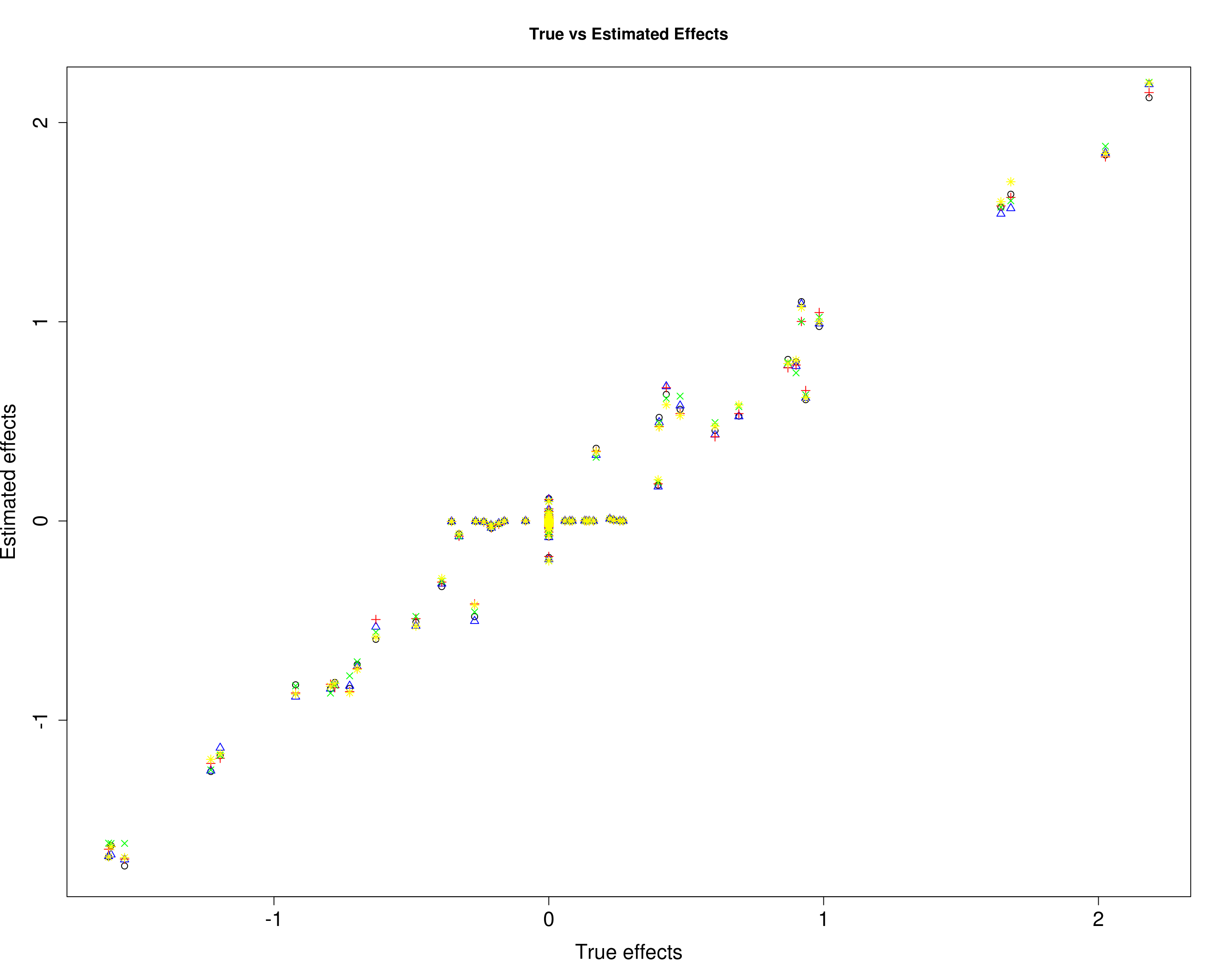
Then, we compare the predicted responses with the true responses in the training data (left panel) and test data (right panel).
par(mfrow=c(1,2))
plot(Ytrain1[, 1], fitted1[, 1], xlab="True responses", ylab="Fitted values", main="True vs Fitted values \nTraining data", pch=1, cex.lab=1.5, cex.axis=1.5)
points(Ytrain1[, 2], fitted1[, 2], col="blue", pch=2)
points(Ytrain1[, 3], fitted1[, 3], col="red", pch=3)
points(Ytrain1[, 4], fitted1[, 4], col="green", pch=4)
points(Ytrain1[, 5], fitted1[, 5], col="yellow", pch=8)
abline(0, 1)

plot(Ytrain1[, 1], fitted1[, 1], xlab="True responses", ylab="Predicted responses", main="True vs Predicted Responses \nTest data", pch=1, cex.lab=1.5, cex.axis=1.5)
points(Ytest1[, 2], Yhat_test1[, 2], col="blue", pch=2)
points(Ytest1[, 3], Yhat_test1[, 3], col="red", pch=3)
points(Ytest1[, 4], Yhat_test1[, 4], col="green", pch=4)
points(Ytest1[, 5], Yhat_test1[, 5], col="yellow", pch=8)
abline(0, 1)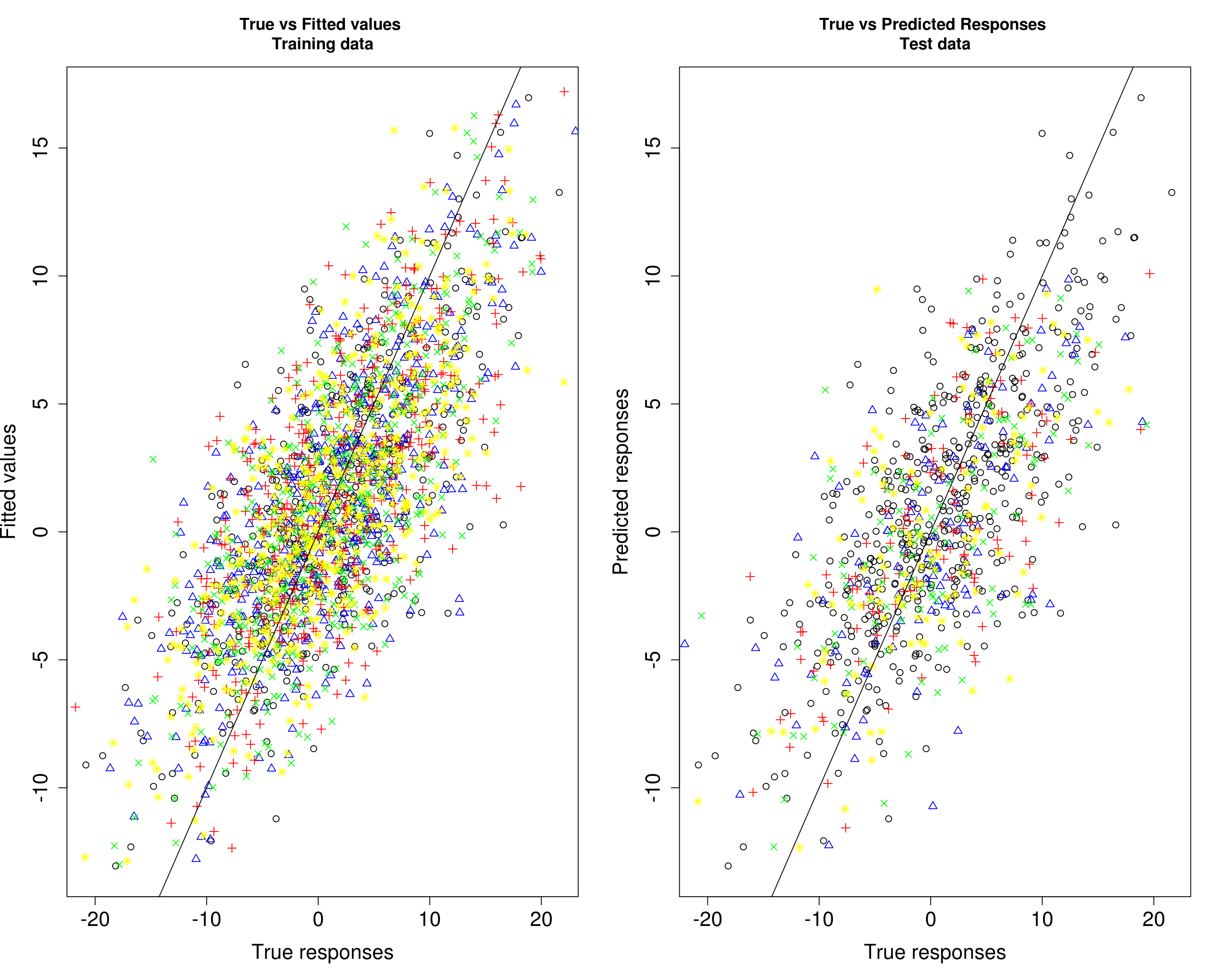
par(mfrow=c(1,1))

r2_train1 <- round(accuracy(Ytrain1, fitted1)$r2, 4)
r2_test1 <- round(accuracy(Ytest1, Yhat_test1)$r2, 4)
bias_train1 <- round(accuracy(Ytrain1, fitted1)$bias, 4)
bias_test1 <- round(accuracy(Ytest1, Yhat_test1)$bias, 4)
mse_train1 <- round(accuracy(Ytrain1, fitted1)$mse, 4)
mse_test1 <- round(accuracy(Ytest1, Yhat_test1)$mse, 4)

acc1 <- rbind(r2_train1, r2_test1, bias_train1, bias_test1, mse_train1, mse_test1)
colnames(acc1) <- paste0("Y", seq(1, r1))
part_metric1 <- c("Training data r2", "Test data r2", "Training data bias", "Test data bias" , "Training data MSE" , "Test data MSE")
res1 <- data.frame(part_metric1, acc1)
colnames(res1)[1] <- c("Partition_metric")
rownames(res1) <- NULL
print(res1)
Partition_metric Y1 Y2 Y3 Y4 Y5
1 Training data r2 0.5338 0.5418 0.4904 0.5239 0.5620
2 Test data r2 0.4591 0.4476 0.4630 0.4523 0.4237
3 Training data bias 1.0606 1.0586 0.9935 1.0013 1.0971
4 Test data bias 0.9892 1.0660 1.0666 1.0905 0.9659
5 Training data MSE 24.6985 23.8540 25.3913 22.4603 23.9106
6 Test data MSE 24.5054 29.4890 27.1642 29.6734 26.7496Simulation 2 – Independent effects, independent variables
dat2 <- readRDS("output/fit_mr_mash_n600_p1000_p_caus50_r5_pve0.5_sigmaoffdiag0_sigmascale0.8_gammaoffdiag0_gammascale0.8_Voffdiag0.2_Vscale0_updatew0TRUE_updatew0TRUE_updatew0methodmixsqp_updateVTRUE.rds")
n2 <- dat2$params$n
p2 <- dat2$params$p
p_causal2 <- dat2$params$p_causal
r2 <- dat2$params$r
k2 <- length(dat2$fit$w0)
pve2 <- dat2$params$pve
prop_testset2 <- dat2$params$prop_testset
B2 <- dat2$inputs$B
V2 <- dat2$inputs$V
Sigma2 <- dat2$inputs$Sigma
Gamma2 <- dat2$inputs$Gamma
Ytrain2 <- dat2$Ytrain
Ytest2 <- dat2$Ytest
mu12 <- dat2$fit$mu1
fitted2 <- dat2$fit$fitted
Yhat_test2 <- dat2$Yhat_test
The results below are based on simulation with 600 samples, 1000 variables of which 50 were causal, 5 responses with a per-response proportion of variance explained (PVE) of 0.5. Variables, X, were drawn from MVN(0, Gamma), causal effects, B, were drawn from MVN(0, Sigma). The responses, Y, were drawn from MN(XB, I, V).
cat("Gamma (First 5 elements)")Gamma (First 5 elements)Gamma2[1:5, 1:5] [,1] [,2] [,3] [,4] [,5]
[1,] 0.8 0.0 0.0 0.0 0.0
[2,] 0.0 0.8 0.0 0.0 0.0
[3,] 0.0 0.0 0.8 0.0 0.0
[4,] 0.0 0.0 0.0 0.8 0.0
[5,] 0.0 0.0 0.0 0.0 0.8cat("Sigma")SigmaSigma2 [,1] [,2] [,3] [,4] [,5]
[1,] 0.8 0.0 0.0 0.0 0.0
[2,] 0.0 0.8 0.0 0.0 0.0
[3,] 0.0 0.0 0.8 0.0 0.0
[4,] 0.0 0.0 0.0 0.8 0.0
[5,] 0.0 0.0 0.0 0.0 0.8cat("V")VV2 [,1] [,2] [,3] [,4] [,5]
[1,] 39.87305 0.00000 0.00000 0.00000 0.00000
[2,] 0.00000 24.41042 0.00000 0.00000 0.00000
[3,] 0.00000 0.00000 27.69452 0.00000 0.00000
[4,] 0.00000 0.00000 0.00000 25.53166 0.00000
[5,] 0.00000 0.00000 0.00000 0.00000 29.00472mr.mash was fitted to the training data (80% of the data) updating V and updating the prior weights using mixSQP. Then, responses were predicted on the test data (20% of the data). The mixture prior consisted of 101 components.
In the plots below, each color/symbol defines a diffrent response.
Here, we compare the estimated effects with the true effects.
plot(B2[, 1], mu12[, 1], xlab="True effects", ylab="Estimated effects", main="True vs Estimated Effects", pch=1, cex.lab=1.5, cex.axis=1.5)
points(B2[, 2], mu12[, 2], col="blue", pch=2)
points(B2[, 3], mu12[, 3], col="red", pch=3)
points(B2[, 4], mu12[, 4], col="green", pch=4)
points(B2[, 5], mu12[, 5], col="yellow", pch=8)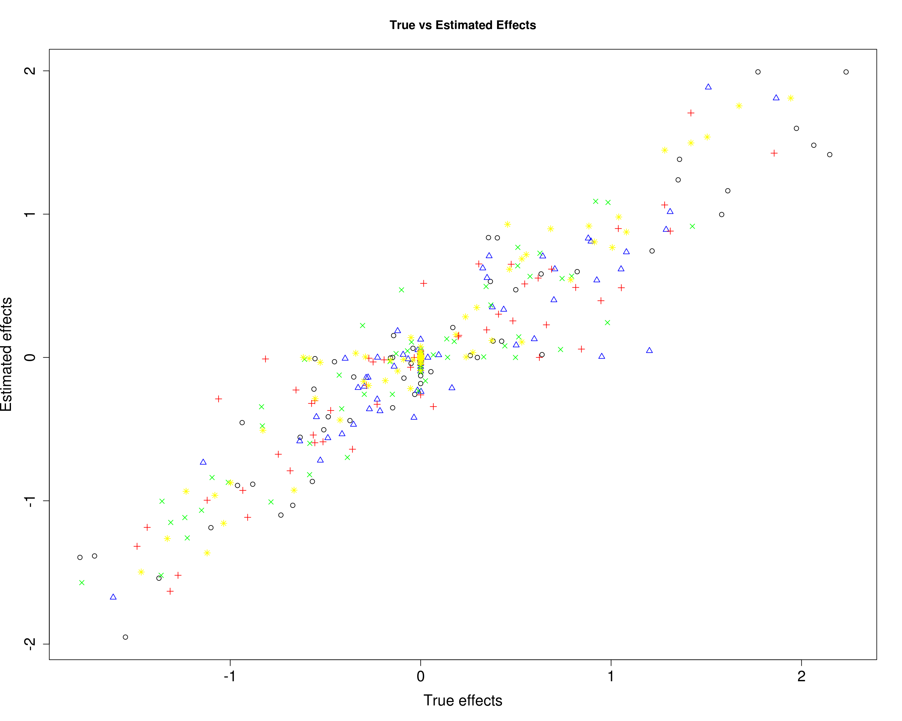
Then, we compare the predicted responses with the true responses in the training data (left panel) and test data (right panel).
par(mfrow=c(1,2))
plot(Ytrain2[, 1], fitted2[, 1], xlab="True responses", ylab="Fitted values", main="True vs Fitted values \nTraining data", pch=1, cex.lab=1.5, cex.axis=1.5)
points(Ytrain2[, 2], fitted2[, 2], col="blue", pch=2)
points(Ytrain2[, 3], fitted2[, 3], col="red", pch=3)
points(Ytrain2[, 4], fitted2[, 4], col="green", pch=4)
points(Ytrain2[, 5], fitted2[, 5], col="yellow", pch=8)
abline(0, 1)

plot(Ytrain2[, 1], fitted2[, 1], xlab="True responses", ylab="Predicted responses", main="True vs Predicted Responses \nTest data", pch=1, cex.lab=1.5, cex.axis=1.5)
points(Ytest2[, 2], Yhat_test2[, 2], col="blue", pch=2)
points(Ytest2[, 3], Yhat_test2[, 3], col="red", pch=3)
points(Ytest2[, 4], Yhat_test2[, 4], col="green", pch=4)
points(Ytest2[, 5], Yhat_test2[, 5], col="yellow", pch=8)
abline(0, 1)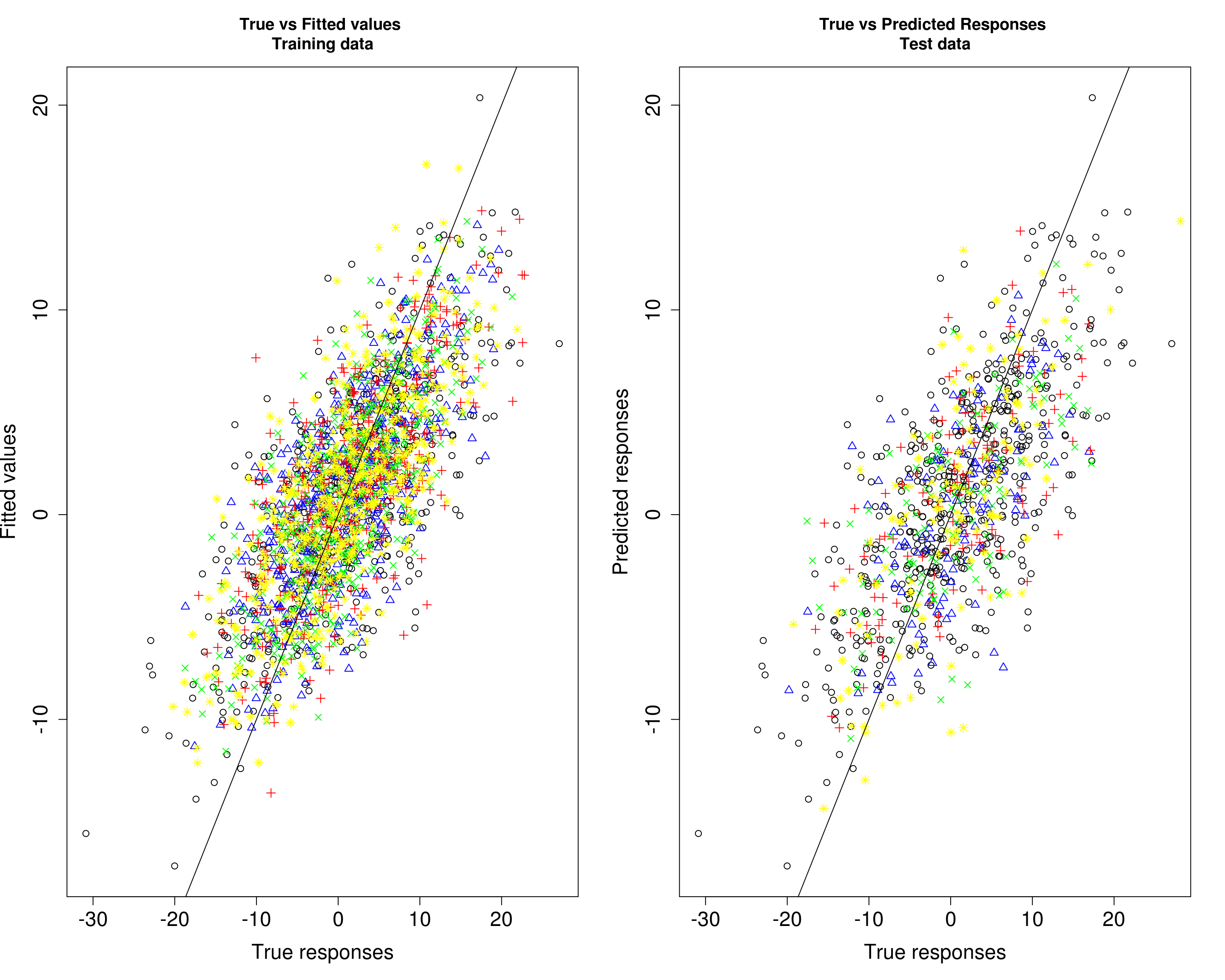
par(mfrow=c(1,1))

r2_train2 <- round(accuracy(Ytrain2, fitted2)$r2, 4)
r2_test2 <- round(accuracy(Ytest2, Yhat_test2)$r2, 4)
bias_train2 <- round(accuracy(Ytrain2, fitted2)$bias, 4)
bias_test2 <- round(accuracy(Ytest2, Yhat_test2)$bias, 4)
mse_train2 <- round(accuracy(Ytrain2, fitted2)$mse, 4)
mse_test2 <- round(accuracy(Ytest2, Yhat_test2)$mse, 4)

acc2 <- rbind(r2_train2, r2_test2, bias_train2, bias_test2, mse_train2, mse_test2)
colnames(acc2) <- paste0("Y", seq(1, r2))
part_metric2 <- c("Training data r2", "Test data r2", "Training data bias", "Test data bias" , "Training data MSE" , "Test data MSE")
res2 <- data.frame(part_metric2, acc2)
colnames(res2)[1] <- c("Partition_metric")
rownames(res2) <- NULL
print(res2)
Partition_metric Y1 Y2 Y3 Y4 Y5
1 Training data r2 0.5373 0.5341 0.5146 0.5716 0.5570
2 Test data r2 0.4600 0.3854 0.4395 0.4473 0.4948
3 Training data bias 1.1737 1.1069 1.1264 1.1019 1.1270
4 Test data bias 0.9847 0.9370 1.1124 1.1859 0.9449
5 Training data MSE 38.1690 22.6568 25.8972 21.0610 26.7705
6 Test data MSE 41.8959 28.1329 34.3800 34.3338 30.6942Simulation 3 – Shared effects, correlated variables
dat3 <- readRDS("output/fit_mr_mash_n600_p1000_p_caus50_r5_pve0.5_sigmaoffdiag1_sigmascale0.8_gammaoffdiag0.5_gammascale0.8_Voffdiag0.2_Vscale0_updatew0TRUE_updatew0TRUE_updatew0methodmixsqp_updateVTRUE.rds")
n3 <- dat3$params$n
p3 <- dat3$params$p
p_causal3 <- dat3$params$p_causal
r3 <- dat3$params$r
k3 <- length(dat3$fit$w0)
pve3 <- dat3$params$pve
prop_testset3 <- dat3$params$prop_testset
B3 <- dat3$inputs$B
V3 <- dat3$inputs$V
Sigma3 <- dat3$inputs$Sigma
Gamma3 <- dat3$inputs$Gamma
Ytrain3 <- dat3$Ytrain
Ytest3 <- dat3$Ytest
mu13 <- dat3$fit$mu1
fitted3 <- dat3$fit$fitted
Yhat_test3 <- dat3$Yhat_test
The results below are based on simulation with 600 samples, 1000 variables of which 50 were causal, 5 responses with a per-response proportion of variance explained (PVE) of 0.5. Variables, X, were drawn from MVN(0, Gamma), causal effects, B, were drawn from MVN(0, Sigma). The responses, Y, were drawn from MN(XB, I, V).
cat("Gamma (First 5 elements)")Gamma (First 5 elements)Gamma3[1:5, 1:5] [,1] [,2] [,3] [,4] [,5]
[1,] 0.8 0.4 0.4 0.4 0.4
[2,] 0.4 0.8 0.4 0.4 0.4
[3,] 0.4 0.4 0.8 0.4 0.4
[4,] 0.4 0.4 0.4 0.8 0.4
[5,] 0.4 0.4 0.4 0.4 0.8cat("Sigma")SigmaSigma3 [,1] [,2] [,3] [,4] [,5]
[1,] 0.8 0.8 0.8 0.8 0.8
[2,] 0.8 0.8 0.8 0.8 0.8
[3,] 0.8 0.8 0.8 0.8 0.8
[4,] 0.8 0.8 0.8 0.8 0.8
[5,] 0.8 0.8 0.8 0.8 0.8cat("V")VV3 [,1] [,2] [,3] [,4] [,5]
[1,] 13.98626 0.00000 0.00000 0.00000 0.00000
[2,] 0.00000 13.98625 0.00000 0.00000 0.00000
[3,] 0.00000 0.00000 13.98625 0.00000 0.00000
[4,] 0.00000 0.00000 0.00000 13.98625 0.00000
[5,] 0.00000 0.00000 0.00000 0.00000 13.98625mr.mash was fitted to the training data (80% of the data) updating V and updating the prior weights using mixSQP. Then, responses were predicted on the test data (20% of the data). The mixture prior consisted of 101 components.
In the plots below, each color/symbol defines a diffrent response.
Here, we compare the estimated effects with the true effects.
plot(B3[, 1], mu13[, 1], xlab="True effects", ylab="Estimated effects", main="True vs Estimated Effects", pch=1, cex.lab=1.5, cex.axis=1.5)
points(B3[, 2], mu13[, 2], col="blue", pch=2)
points(B3[, 3], mu13[, 3], col="red", pch=3)
points(B3[, 4], mu13[, 4], col="green", pch=4)
points(B3[, 5], mu13[, 5], col="yellow", pch=8)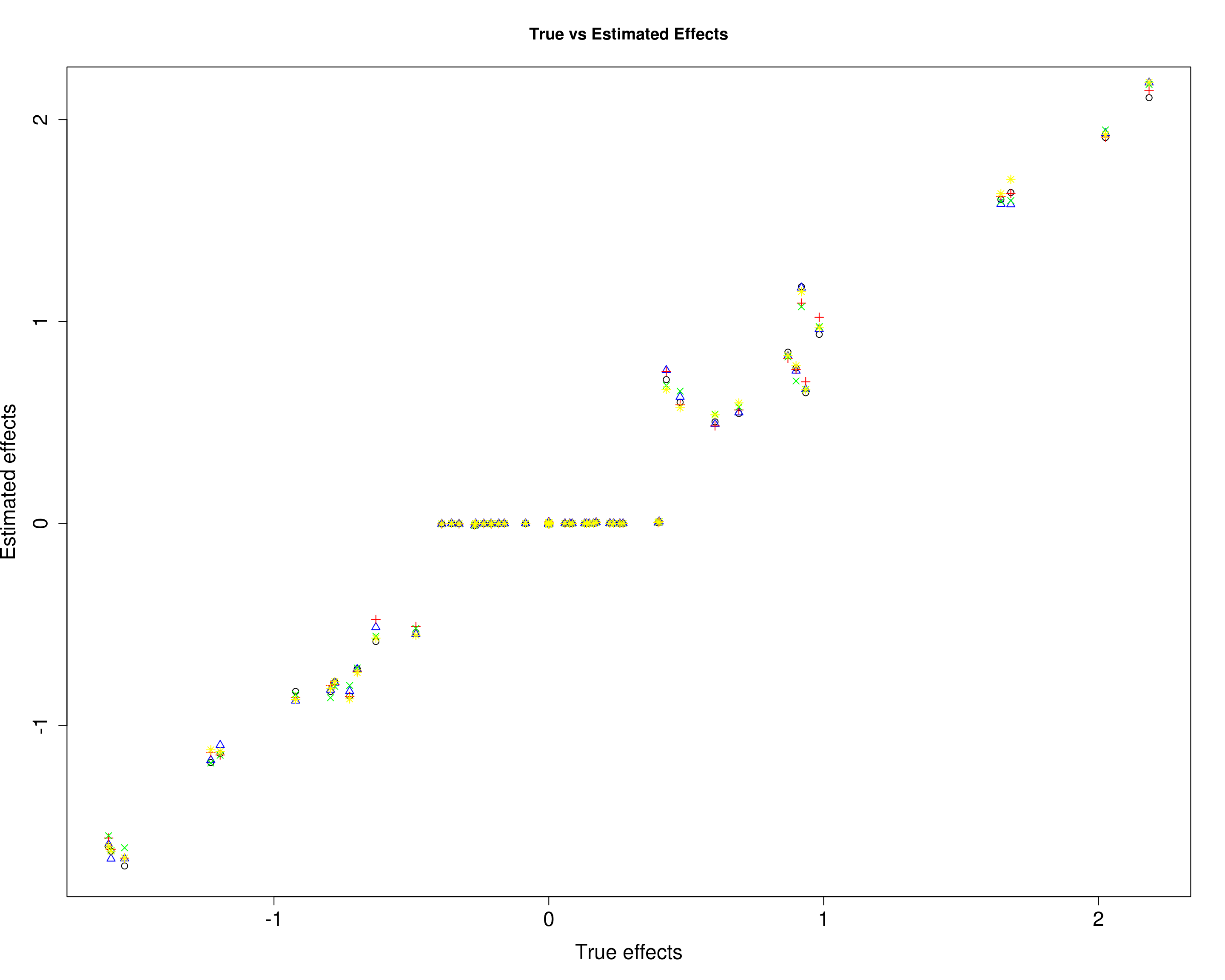
Then, we compare the predicted responses with the true responses in the training data (left panel) and test data (right panel).
par(mfrow=c(1,2))
plot(Ytrain3[, 1], fitted3[, 1], xlab="True responses", ylab="Fitted values", main="True vs Fitted values \nTraining data", pch=1, cex.lab=1.5, cex.axis=1.5)
points(Ytrain3[, 2], fitted3[, 2], col="blue", pch=2)
points(Ytrain3[, 3], fitted3[, 3], col="red", pch=3)
points(Ytrain3[, 4], fitted3[, 4], col="green", pch=4)
points(Ytrain3[, 5], fitted3[, 5], col="yellow", pch=8)
abline(0, 1)

plot(Ytrain3[, 1], fitted3[, 1], xlab="True responses", ylab="Predicted responses", main="True vs Predicted Responses \nTest data", pch=1, cex.lab=1.5, cex.axis=1.5)
points(Ytest3[, 2], Yhat_test3[, 2], col="blue", pch=2)
points(Ytest3[, 3], Yhat_test3[, 3], col="red", pch=3)
points(Ytest3[, 4], Yhat_test3[, 4], col="green", pch=4)
points(Ytest3[, 5], Yhat_test3[, 5], col="yellow", pch=8)
abline(0, 1)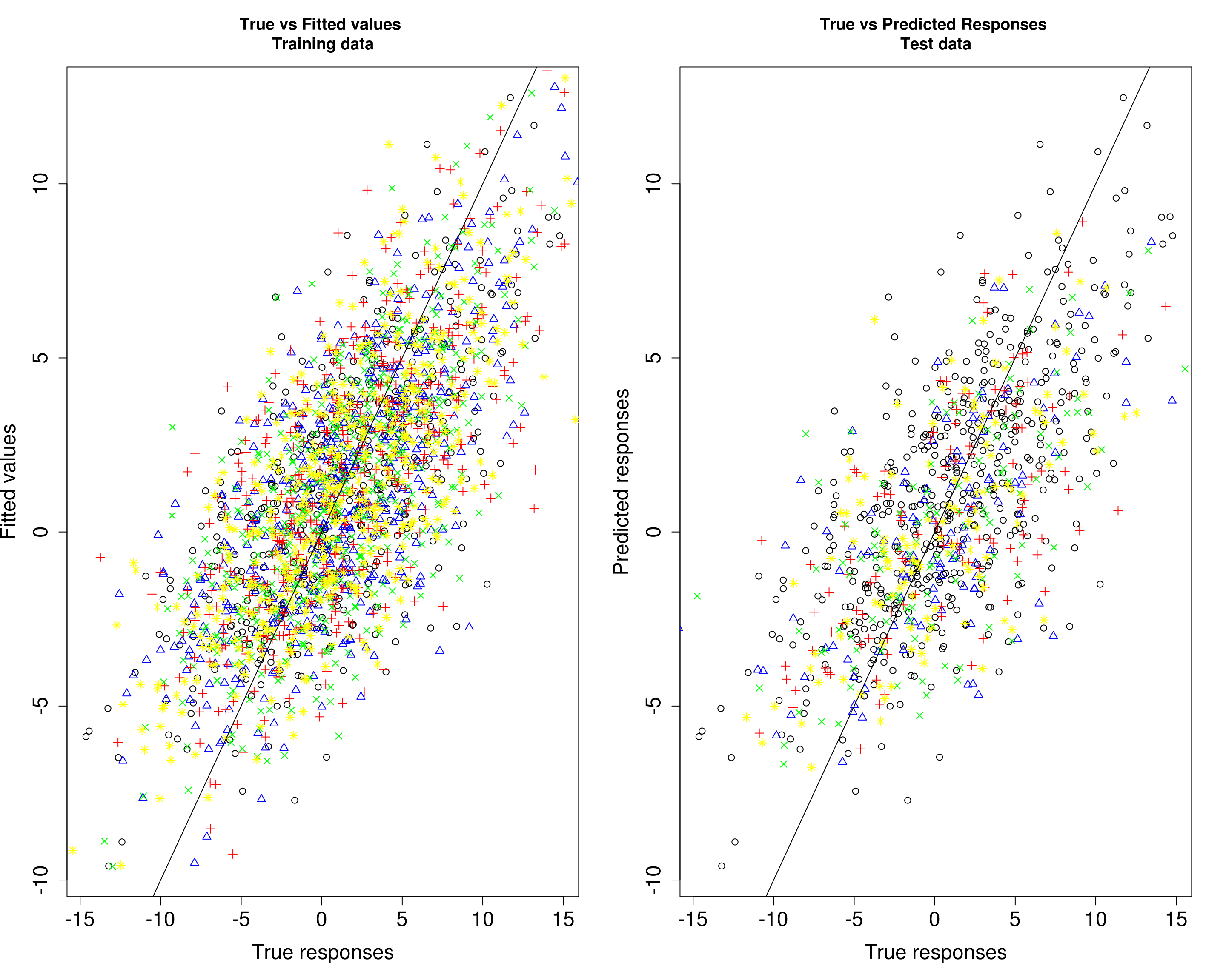
par(mfrow=c(1,1))

r2_train3 <- round(accuracy(Ytrain3, fitted3)$r2, 4)
r2_test3 <- round(accuracy(Ytest3, Yhat_test3)$r2, 4)
bias_train3 <- round(accuracy(Ytrain3, fitted3)$bias, 4)
bias_test3 <- round(accuracy(Ytest3, Yhat_test3)$bias, 4)
mse_train3 <- round(accuracy(Ytrain3, fitted3)$mse, 4)
mse_test3 <- round(accuracy(Ytest3, Yhat_test3)$mse, 4)

acc3 <- rbind(r2_train3, r2_test3, bias_train3, bias_test3, mse_train3, mse_test3)
colnames(acc3) <- paste0("Y", seq(1, r3))
part_metric3 <- c("Training data r2", "Test data r2", "Training data bias", "Test data bias" , "Training data MSE" , "Test data MSE")
res3 <- data.frame(part_metric3, acc3)
colnames(res3)[1] <- c("Partition_metric")
rownames(res3) <- NULL
print(res3)
Partition_metric Y1 Y2 Y3 Y4 Y5
1 Training data r2 0.4892 0.5037 0.4710 0.4907 0.5390
2 Test data r2 0.4148 0.4341 0.4220 0.4639 0.4251
3 Training data bias 1.0358 1.0376 0.9876 0.9817 1.0887
4 Test data bias 1.0015 1.0979 1.0552 1.1736 1.0079
5 Training data MSE 14.4128 14.0238 14.5096 12.8917 13.6560
6 Test data MSE 14.0750 15.9244 15.3882 15.9627 14.0499Simulation 4 – Independent effects, correlated variables
dat4 <- readRDS("output/fit_mr_mash_n600_p1000_p_caus50_r5_pve0.5_sigmaoffdiag0_sigmascale0.8_gammaoffdiag0.5_gammascale0.8_Voffdiag0.2_Vscale0_updatew0TRUE_updatew0TRUE_updatew0methodmixsqp_updateVTRUE.rds")
n4 <- dat4$params$n
p4 <- dat4$params$p
p_causal4 <- dat4$params$p_causal
r4 <- dat4$params$r
k4 <- length(dat4$fit$w0)
pve4 <- dat4$params$pve
prop_testset4 <- dat4$params$prop_testset
B4 <- dat4$inputs$B
V4 <- dat4$inputs$V
Sigma4 <- dat4$inputs$Sigma
Gamma4 <- dat4$inputs$Gamma
Ytrain4 <- dat4$Ytrain
Ytest4 <- dat4$Ytest
mu14 <- dat4$fit$mu1
fitted4 <- dat4$fit$fitted
Yhat_test4 <- dat4$Yhat_test
The results below are based on simulation with 600 samples, 1000 variables of which 50 were causal, 5 responses with a per-response proportion of variance explained (PVE) of 0.5. Variables, X, were drawn from MVN(0, Gamma), causal effects, B, were drawn from MVN(0, Sigma). The responses, Y, were drawn from MN(XB, I, V).
cat("Gamma (First 5 elements)")Gamma (First 5 elements)Gamma4[1:5, 1:5] [,1] [,2] [,3] [,4] [,5]
[1,] 0.8 0.4 0.4 0.4 0.4
[2,] 0.4 0.8 0.4 0.4 0.4
[3,] 0.4 0.4 0.8 0.4 0.4
[4,] 0.4 0.4 0.4 0.8 0.4
[5,] 0.4 0.4 0.4 0.4 0.8cat("Sigma")SigmaSigma4 [,1] [,2] [,3] [,4] [,5]
[1,] 0.8 0.0 0.0 0.0 0.0
[2,] 0.0 0.8 0.0 0.0 0.0
[3,] 0.0 0.0 0.8 0.0 0.0
[4,] 0.0 0.0 0.0 0.8 0.0
[5,] 0.0 0.0 0.0 0.0 0.8cat("V")VV4 [,1] [,2] [,3] [,4] [,5]
[1,] 31.75545 0.00000 0.00000 0.00000 0.00000
[2,] 0.00000 31.47091 0.00000 0.00000 0.00000
[3,] 0.00000 0.00000 14.55202 0.00000 0.00000
[4,] 0.00000 0.00000 0.00000 42.12604 0.00000
[5,] 0.00000 0.00000 0.00000 0.00000 15.37456mr.mash was fitted to the training data (80% of the data) updating V and updating the prior weights using mixSQP. Then, responses were predicted on the test data (20% of the data). The mixture prior consisted of 101 components.
In the plots below, each color/symbol defines a diffrent response.
Here, we compare the estimated effects with the true effects.
plot(B4[, 1], mu14[, 1], xlab="True effects", ylab="Estimated effects", main="True vs Estimated Effects", pch=1, cex.lab=1.5, cex.axis=1.5)
points(B4[, 2], mu14[, 2], col="blue", pch=2)
points(B4[, 3], mu14[, 3], col="red", pch=3)
points(B4[, 4], mu14[, 4], col="green", pch=4)
points(B4[, 5], mu14[, 5], col="yellow", pch=8)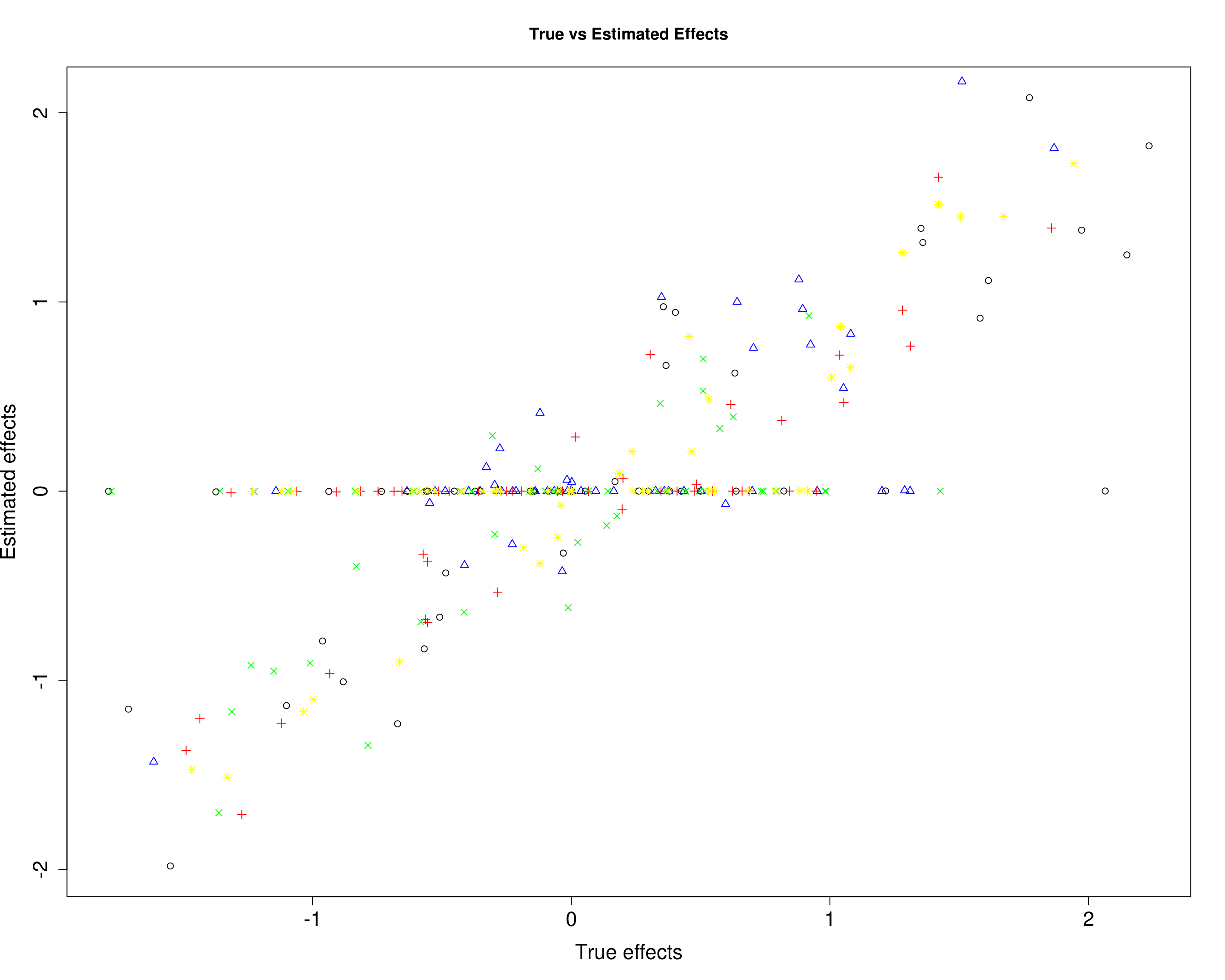
Then, we compare the predicted responses with the true responses in the training data (left panel) and test data (right panel).
par(mfrow=c(1,2))
plot(Ytrain4[, 1], fitted4[, 1], xlab="True responses", ylab="Fitted values", main="True vs Fitted values \nTraining data", pch=1, cex.lab=1.5, cex.axis=1.5)
points(Ytrain4[, 2], fitted4[, 2], col="blue", pch=2)
points(Ytrain4[, 3], fitted4[, 3], col="red", pch=3)
points(Ytrain4[, 4], fitted4[, 4], col="green", pch=4)
points(Ytrain4[, 5], fitted4[, 5], col="yellow", pch=8)
abline(0, 1)

plot(Ytrain4[, 1], fitted4[, 1], xlab="True responses", ylab="Predicted responses", main="True vs Predicted Responses \nTest data", pch=1, cex.lab=1.5, cex.axis=1.5)
points(Ytest4[, 2], Yhat_test4[, 2], col="blue", pch=2)
points(Ytest4[, 3], Yhat_test4[, 3], col="red", pch=3)
points(Ytest4[, 4], Yhat_test4[, 4], col="green", pch=4)
points(Ytest4[, 5], Yhat_test4[, 5], col="yellow", pch=8)
abline(0, 1)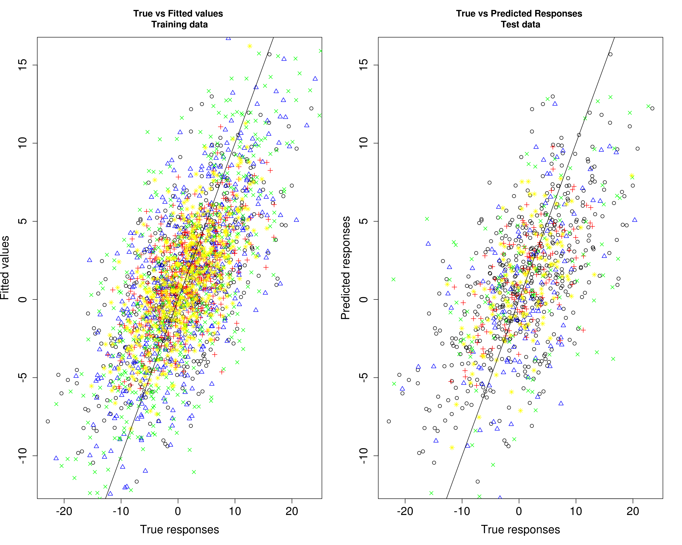
par(mfrow=c(1,1))

r2_train4 <- round(accuracy(Ytrain4, fitted4)$r2, 4)
r2_test4 <- round(accuracy(Ytest4, Yhat_test4)$r2, 4)
bias_train4 <- round(accuracy(Ytrain4, fitted4)$bias, 4)
bias_test4 <- round(accuracy(Ytest4, Yhat_test4)$bias, 4)
mse_train4 <- round(accuracy(Ytrain4, fitted4)$mse, 4)
mse_test4 <- round(accuracy(Ytest4, Yhat_test4)$mse, 4)

acc4 <- rbind(r2_train4, r2_test4, bias_train4, bias_test4, mse_train4, mse_test4)
colnames(acc4) <- paste0("Y", seq(1, r4))
part_metric4 <- c("Training data r2", "Test data r2", "Training data bias", "Test data bias" , "Training data MSE" , "Test data MSE")
res4 <- data.frame(part_metric4, acc4)
colnames(res4)[1] <- c("Partition_metric")
rownames(res4) <- NULL
print(res4)
Partition_metric Y1 Y2 Y3 Y4 Y5
1 Training data r2 0.4107 0.4811 0.3574 0.5330 0.4272
2 Test data r2 0.3990 0.2959 0.3766 0.3298 0.3542
3 Training data bias 1.1022 1.0512 1.0676 1.0356 1.0803
4 Test data bias 1.0478 0.7843 1.1576 0.9455 0.9463
5 Training data MSE 36.2095 32.5375 17.8351 39.5427 18.2162
6 Test data MSE 36.5641 38.1858 20.4419 62.0936 19.4614
sessionInfo()R version 3.5.1 (2018-07-02)
Platform: x86_64-pc-linux-gnu (64-bit)
Running under: Scientific Linux 7.4 (Nitrogen)
Matrix products: default
BLAS/LAPACK: /software/openblas-0.2.19-el7-x86_64/lib/libopenblas_haswellp-r0.2.19.so
locale:
[1] LC_CTYPE=en_US.UTF-8 LC_NUMERIC=C
[3] LC_TIME=en_US.UTF-8 LC_COLLATE=en_US.UTF-8
[5] LC_MONETARY=en_US.UTF-8 LC_MESSAGES=en_US.UTF-8
[7] LC_PAPER=en_US.UTF-8 LC_NAME=C
[9] LC_ADDRESS=C LC_TELEPHONE=C
[11] LC_MEASUREMENT=en_US.UTF-8 LC_IDENTIFICATION=C
attached base packages:
[1] stats graphics grDevices utils datasets methods base
loaded via a namespace (and not attached):
[1] workflowr_1.6.1 Rcpp_1.0.3 digest_0.6.25 later_0.7.5
[5] rprojroot_1.3-2 R6_2.4.1 backports_1.1.5 git2r_0.26.1
[9] magrittr_1.5 evaluate_0.12 stringi_1.4.3 fs_1.3.1
[13] promises_1.0.1 whisker_0.3-2 rmarkdown_1.10 tools_3.5.1
[17] stringr_1.4.0 glue_1.4.0 httpuv_1.4.5 yaml_2.2.1
[21] compiler_3.5.1 htmltools_0.3.6 knitr_1.20