Dense case
Fabio Morgante
June 02, 2020
Last updated: 2020-06-02
Checks: 7 0
Knit directory: mr_mash_test/
This reproducible R Markdown analysis was created with workflowr (version 1.6.1). The Checks tab describes the reproducibility checks that were applied when the results were created. The Past versions tab lists the development history.
Great! Since the R Markdown file has been committed to the Git repository, you know the exact version of the code that produced these results.
Great job! The global environment was empty. Objects defined in the global environment can affect the analysis in your R Markdown file in unknown ways. For reproduciblity it’s best to always run the code in an empty environment.
The command set.seed(20200328) was run prior to running the code in the R Markdown file. Setting a seed ensures that any results that rely on randomness, e.g. subsampling or permutations, are reproducible.
Great job! Recording the operating system, R version, and package versions is critical for reproducibility.
Nice! There were no cached chunks for this analysis, so you can be confident that you successfully produced the results during this run.
Great job! Using relative paths to the files within your workflowr project makes it easier to run your code on other machines.
Great! You are using Git for version control. Tracking code development and connecting the code version to the results is critical for reproducibility.
The results in this page were generated with repository version 2851240. See the Past versions tab to see a history of the changes made to the R Markdown and HTML files.
Note that you need to be careful to ensure that all relevant files for the analysis have been committed to Git prior to generating the results (you can use wflow_publish or wflow_git_commit). workflowr only checks the R Markdown file, but you know if there are other scripts or data files that it depends on. Below is the status of the Git repository when the results were generated:
Ignored files:
    Ignored:    .sos/
    Ignored:    code/fit_mr_mash.66662433.err
    Ignored:    code/fit_mr_mash.66662433.out
    Ignored:    dsc/.sos/
    Ignored:    dsc/outfiles/
    Ignored:    output/dsc.html
    Ignored:    output/dsc/
    Ignored:    output/dsc_05_18_20.html
    Ignored:    output/dsc_05_18_20/
    Ignored:    output/dsc_05_29_20.html
    Ignored:    output/dsc_05_29_20/
    Ignored:    output/dsc_OLD.html
    Ignored:    output/dsc_OLD/
    Ignored:    output/dsc_test.html
    Ignored:    output/dsc_test/

Untracked files:
    Untracked:  code/plot_test.R

Unstaged changes:
    Modified:   dsc/midway2.yml
Note that any generated files, e.g. HTML, png, CSS, etc., are not included in this status report because it is ok for generated content to have uncommitted changes.
These are the previous versions of the repository in which changes were made to the R Markdown (analysis/dense_scenario_issue.Rmd) and HTML (docs/dense_scenario_issue.html) files. If you’ve configured a remote Git repository (see ?wflow_git_remote), click on the hyperlinks in the table below to view the files as they were in that past version.
| File | Version | Author | Date | Message |
|---|---|---|---|---|
| Rmd | 2851240 | fmorgante | 2020-06-02 | Fix bug in dense scenario |
| html | 5328c22 | fmorgante | 2020-06-02 | Build site. |
| Rmd | 3c70b54 | fmorgante | 2020-06-02 | Update dense scenario |
| html | 2ace633 | fmorgante | 2020-06-02 | Build site. |
| Rmd | 654b67a | fmorgante | 2020-06-02 | Add additional simulation to the dense scenario |
| html | 42ec51c | fmorgante | 2020-06-01 | Build site. |
| Rmd | ceda278 | fmorgante | 2020-06-01 | Add case study with dense scenario |
library(mr.mash.alpha)
library(glmnet)
Loading required package: MatrixLoading required package: foreachLoaded glmnet 2.0-16###Set options
options(stringsAsFactors = FALSE)
###Function to compute accuracy
compute_accuracy <- function(Y, Yhat) {
bias <- rep(as.numeric(NA), ncol(Y))
r2 <- rep(as.numeric(NA), ncol(Y))
mse <- rep(as.numeric(NA), ncol(Y))
for(i in 1:ncol(Y)){
fit <- lm(Y[, i] ~ Yhat[, i])
bias[i] <- coef(fit)[2]
r2[i] <- summary(fit)$r.squared
mse[i] <- mean((Y[, i] - Yhat[, i])^2)
}
return(list(bias=bias, r2=r2, mse=mse))
}Dense scenario
Here we investigate why mr.mash does not perform as well in denser scenarios. Let’s simulate data with n=600, p=1,000, p_causal=500, r=5, r_causal=5, PVE=0.5, shared effects, independent predictors, and independent residuals. The models will be fitted to the training data (80% of the full data).
###Set seed
set.seed(123)

###Set parameters
n <- 600
p <- 1000
p_causal <- 500
r <- 5
r_causal <- r
pve <- 0.5
B_cor <- 1
X_cor <- 0
V_cor <- 0

###Simulate V, B, X and Y
out <- mr.mash.alpha:::simulate_mr_mash_data(n, p, p_causal, r, r_causal=r, intercepts = rep(1, r),
                                             pve=pve, B_cor=B_cor, B_scale=0.9, X_cor=X_cor, X_scale=0.8, V_cor=V_cor)

colnames(out$Y) <- paste0("Y", seq(1, r))
rownames(out$Y) <- paste0("N", seq(1, n))
colnames(out$X) <- paste0("X", seq(1, p))
rownames(out$X) <- paste0("N", seq(1, n))

###Split the data in training and test sets
test_set <- sort(sample(x=c(1:n), size=round(n*0.2), replace=FALSE))
Ytrain <- out$Y[-test_set, ]
Xtrain <- out$X[-test_set, ]
Ytest <- out$Y[test_set, ]
Xtest <- out$X[test_set, ]
We build the mixture prior as usual including zero matrix, identity matrix, rank-1 matrices, low, medium and high heterogeneity matrices, shared matrix, each scaled by a grid from 0.1 to 2.1 in steps of 0.2.
grid <- seq(0.1, 2.1, 0.2)
S0 <- mr.mash.alpha:::compute_cov_canonical(ncol(Ytrain), singletons=TRUE, hetgrid=c(0, 0.25, 0.5, 0.75, 1), grid, zeromat=TRUE)
We run glmnet with \(\alpha=1\) to obtain an inital estimate for the regression coefficients to provide to mr.mash, and for comparison.
###Fit group-lasso
cvfit_glmnet <- cv.glmnet(x=Xtrain, y=Ytrain, family="mgaussian", alpha=1)
coeff_glmnet <- coef(cvfit_glmnet, s="lambda.min")
Bhat_glmnet <- matrix(as.numeric(NA), nrow=p, ncol=r)
ahat_glmnet <- vector("numeric", r)
for(i in 1:length(coeff_glmnet)){
  Bhat_glmnet[, i] <- as.vector(coeff_glmnet[[i]])[-1]
  ahat_glmnet[i] <- as.vector(coeff_glmnet[[i]])[1]
}
Yhat_test_glmnet <- drop(predict(cvfit_glmnet, newx=Xtest, s="lambda.min"))
We run mr.mash with EM updates of the mixture weights, updating V, and initializing the regression coefficients with the estimates from glmnet.
###Fit mr.mash
fit_mrmash <- mr.mash(Xtrain, Ytrain, S0, tol=1e-2, convergence_criterion="ELBO", update_w0=TRUE,
                     update_w0_method="EM", compute_ELBO=TRUE, standardize=TRUE, verbose=FALSE, update_V=TRUE,
                     mu1_init = Bhat_glmnet, w0_threshold=1e-8)
Processing the inputs... Done!
Fitting the optimization algorithm... Done!
Processing the outputs... Done!
mr.mash successfully executed in 2.557808 minutes!Yhat_test_mrmash <- predict(fit_mrmash, Xtest)layout(matrix(c(1, 1, 2, 2,
1, 1, 2, 2,
0, 3, 3, 0,
0, 3, 3, 0), 4, 4, byrow = TRUE))
###Plot estimated vs true coeffcients
##mr.mash
plot(out$B, fit_mrmash$mu1, main="mr.mash", xlab="True coefficients", ylab="Estimated coefficients",
cex=2, cex.lab=1.8, cex.main=2, cex.axis=1.8)
##glmnet
plot(out$B, Bhat_glmnet, main="glmnet", xlab="True coefficients", ylab="Estimated coefficients",
cex=2, cex.lab=1.8, cex.main=2, cex.axis=1.8)
###Plot mr.mash vs glmnet estimated coeffcients
colorz <- matrix("black", nrow=p, ncol=r)
zeros <- apply(out$B, 2, function(x) x==0)
for(i in 1:ncol(colorz)){
colorz[zeros[, i], i] <- "red"
}
plot(Bhat_glmnet, fit_mrmash$mu1, main="mr.mash vs glmnet",
xlab="glmnet estimated coefficients", ylab="mr.mash estimated coefficients",
col=colorz, cex=2, cex.lab=1.8, cex.main=2, cex.axis=1.8)
legend("topleft",
legend = c("Non-zero", "Zero"),
col = c("black", "red"),
pch = c(1, 1),
horiz = FALSE,
cex=2) 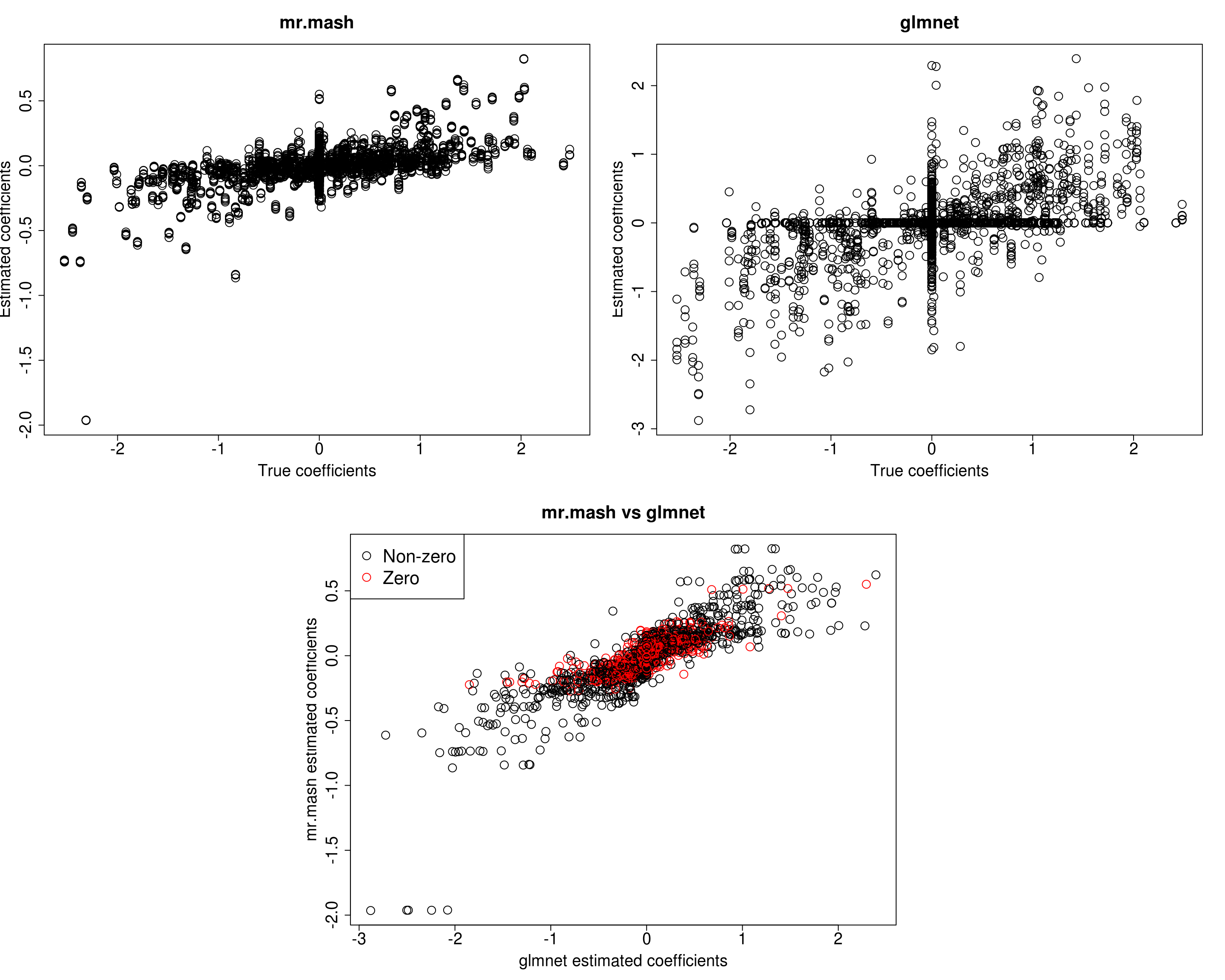
print("Prediction performance with glmnet")[1] "Prediction performance with glmnet"compute_accuracy(Ytest, Yhat_test_glmnet)$bias
[1] 0.7973441 0.7171240 1.1201318 0.9992656 0.9375002
$r2
[1] 0.12560024 0.10044653 0.14357016 0.13204939 0.09516285
$mse
[1] 502.2840 531.2713 573.5326 575.3974 722.7162print("Prediction performance with mr.mash")[1] "Prediction performance with mr.mash"compute_accuracy(Ytest, Yhat_test_mrmash)$bias
[1] 2.268094 2.196013 3.435006 2.831555 3.026599
$r2
[1] 0.1310161 0.1128144 0.2345789 0.1833654 0.1535817
$mse
[1] 518.2328 530.0913 591.4375 587.3239 730.5908print("True V (full data)")[1] "True V (full data)"out$V [,1] [,2] [,3] [,4] [,5]
[1,] 331.4137 0.0000 0.0000 0.0000 0.0000
[2,] 0.0000 331.4137 0.0000 0.0000 0.0000
[3,] 0.0000 0.0000 331.4137 0.0000 0.0000
[4,] 0.0000 0.0000 0.0000 331.4137 0.0000
[5,] 0.0000 0.0000 0.0000 0.0000 331.4137print("Estimated V (training data)")[1] "Estimated V (training data)"fit_mrmash$V Y1 Y2 Y3 Y4 Y5
Y1 600.7891 271.7844 213.0465 197.5704 231.8269
Y2 271.7844 581.4331 244.8055 243.7165 255.7953
Y3 213.0465 244.8055 542.5477 252.0331 239.4896
Y4 197.5704 243.7165 252.0331 532.5570 214.1998
Y5 231.8269 255.7953 239.4896 214.1998 516.2954It looks mr.mash shrinks the coeffcients too much and the residual covariance is absorbing part of the effects. Let’s now try to fix the residual covariance to the truth (although it is going to be a little different since we are fitting the model to the training set only).
###Fit mr.mash
fit_mrmash_fixV <- mr.mash(Xtrain, Ytrain, S0, tol=1e-2, convergence_criterion="ELBO", update_w0=TRUE,
                     update_w0_method="EM", compute_ELBO=TRUE, standardize=TRUE, verbose=FALSE, update_V=FALSE,
                     mu1_init = Bhat_glmnet, w0_threshold=1e-8, V=out$V)
Processing the inputs... Done!
Fitting the optimization algorithm... Done!
Processing the outputs... Done!
mr.mash successfully executed in 3.218407 minutes!Yhat_test_mrmash_fixV <- predict(fit_mrmash_fixV, Xtest)layout(matrix(c(1, 1, 2, 2,
1, 1, 2, 2,
0, 3, 3, 0,
0, 3, 3, 0), 4, 4, byrow = TRUE))
###Plot estimated vs true coeffcients
##mr.mash
plot(out$B, fit_mrmash_fixV$mu1, main="mr.mash", xlab="True coefficients", ylab="Estimated coefficients",
cex=2, cex.lab=1.8, cex.main=2, cex.axis=1.8)
##glmnet
plot(out$B, Bhat_glmnet, main="glmnet", xlab="True coefficients", ylab="Estimated coefficients",
cex=2, cex.lab=1.8, cex.main=2, cex.axis=1.8)
###Plot mr.mash vs glmnet estimated coeffcients
colorz <- matrix("black", nrow=p, ncol=r)
zeros <- apply(out$B, 2, function(x) x==0)
for(i in 1:ncol(colorz)){
colorz[zeros[, i], i] <- "red"
}
plot(Bhat_glmnet, fit_mrmash_fixV$mu1, main="mr.mash vs glmnet",
xlab="glmnet estimated coefficients", ylab="mr.mash estimated coefficients",
col=colorz, cex=2, cex.lab=1.8, cex.main=2, cex.axis=1.8)
legend("topleft",
legend = c("Non-zero", "Zero"),
col = c("black", "red"),
pch = c(1, 1),
horiz = FALSE,
cex=2) 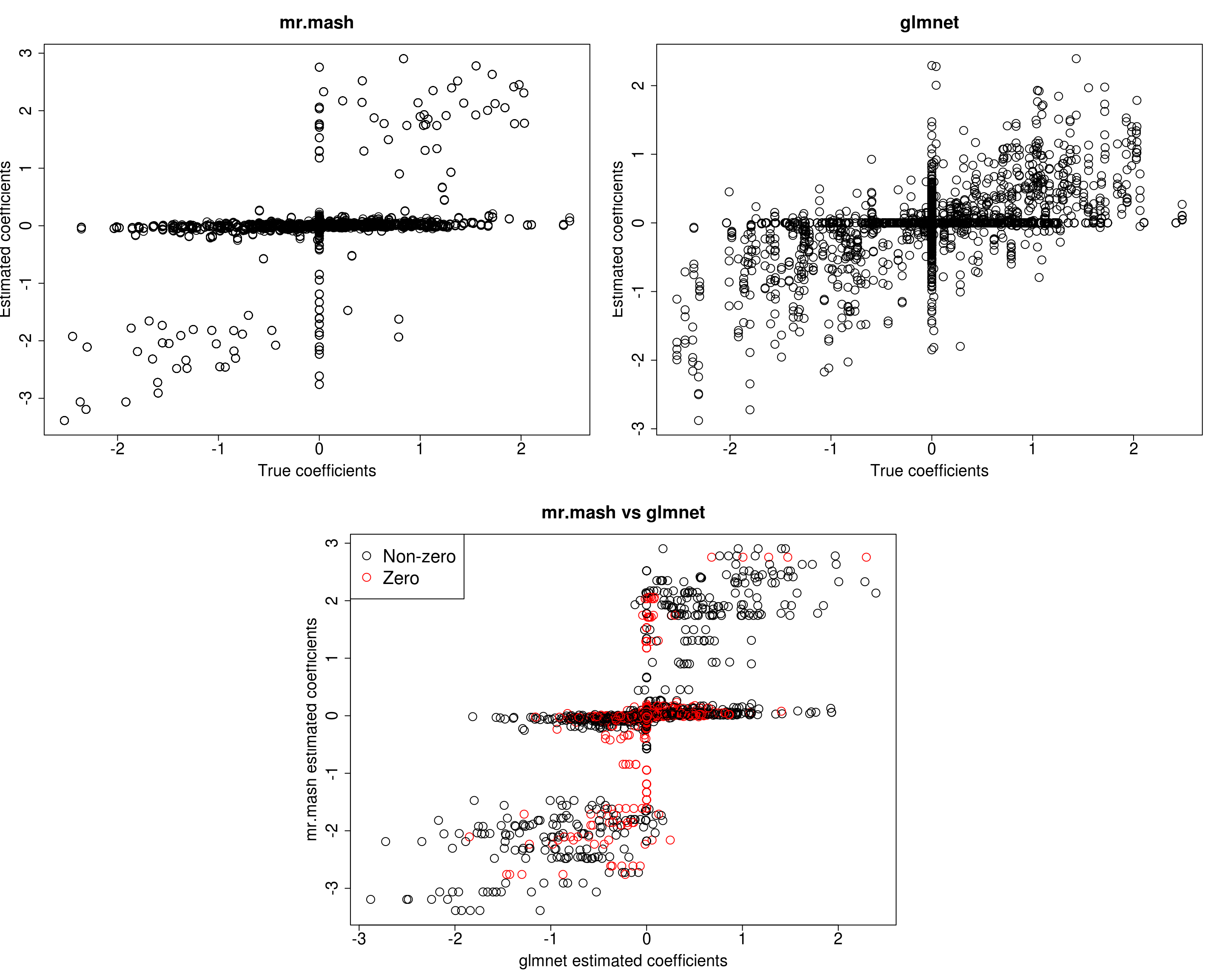
print("Prediction performance with glmnet")[1] "Prediction performance with glmnet"compute_accuracy(Ytest, Yhat_test_glmnet)$bias
[1] 0.7973441 0.7171240 1.1201318 0.9992656 0.9375002
$r2
[1] 0.12560024 0.10044653 0.14357016 0.13204939 0.09516285
$mse
[1] 502.2840 531.2713 573.5326 575.3974 722.7162print("Prediction performance with mr.mash")[1] "Prediction performance with mr.mash"compute_accuracy(Ytest, Yhat_test_mrmash_fixV)$bias
[1] 0.3739759 0.4820432 0.5484524 0.5637339 0.4956777
$r2
[1] 0.07025924 0.11696855 0.12904463 0.13990240 0.08790078
$mse
[1] 642.2267 599.7516 637.9042 632.1933 801.5090Prediction performance looks worse in terms of MSE and \(r^2\) while bias, although still off, is closer to 1. However, looking at the plots of the coefficients, we can see that many coefficients are no longer overshrunk. Let’s see what happens if we initialize V to the truth but then we update it.
###Fit mr.mash
fit_mrmash_initV <- mr.mash(Xtrain, Ytrain, S0, tol=1e-2, convergence_criterion="ELBO", update_w0=TRUE,
                     update_w0_method="EM", compute_ELBO=TRUE, standardize=TRUE, verbose=FALSE, update_V=TRUE,
                     mu1_init = Bhat_glmnet, w0_threshold=1e-8, V=out$V)
Processing the inputs... Done!
Fitting the optimization algorithm... Done!
Processing the outputs... Done!
mr.mash successfully executed in 2.56133 minutes!Yhat_test_mrmash_initV <- predict(fit_mrmash_initV, Xtest)layout(matrix(c(1, 1, 2, 2,
1, 1, 2, 2,
0, 3, 3, 0,
0, 3, 3, 0), 4, 4, byrow = TRUE))
###Plot estimated vs true coeffcients
##mr.mash
plot(out$B, fit_mrmash_initV$mu1, main="mr.mash", xlab="True coefficients", ylab="Estimated coefficients",
cex=2, cex.lab=1.8, cex.main=2, cex.axis=1.8)
##glmnet
plot(out$B, Bhat_glmnet, main="glmnet", xlab="True coefficients", ylab="Estimated coefficients",
cex=2, cex.lab=1.8, cex.main=2, cex.axis=1.8)
###Plot mr.mash vs glmnet estimated coeffcients
colorz <- matrix("black", nrow=p, ncol=r)
zeros <- apply(out$B, 2, function(x) x==0)
for(i in 1:ncol(colorz)){
colorz[zeros[, i], i] <- "red"
}
plot(Bhat_glmnet, fit_mrmash_initV$mu1, main="mr.mash vs glmnet",
xlab="glmnet estimated coefficients", ylab="mr.mash estimated coefficients",
col=colorz, cex=2, cex.lab=1.8, cex.main=2, cex.axis=1.8)
legend("topleft",
legend = c("Non-zero", "Zero"),
col = c("black", "red"),
pch = c(1, 1),
horiz = FALSE,
cex=2) 
print("Prediction performance with glmnet")[1] "Prediction performance with glmnet"compute_accuracy(Ytest, Yhat_test_glmnet)$bias
[1] 0.7973441 0.7171240 1.1201318 0.9992656 0.9375002
$r2
[1] 0.12560024 0.10044653 0.14357016 0.13204939 0.09516285
$mse
[1] 502.2840 531.2713 573.5326 575.3974 722.7162print("Prediction performance with mr.mash")[1] "Prediction performance with mr.mash"compute_accuracy(Ytest, Yhat_test_mrmash_initV)$bias
[1] 2.249720 2.175435 3.415054 2.814300 3.008327
$r2
[1] 0.1300084 0.1116978 0.2339525 0.1826696 0.1530939
$mse
[1] 518.3294 530.2425 591.2687 587.2565 730.4772print("True V (full data)")[1] "True V (full data)"out$V [,1] [,2] [,3] [,4] [,5]
[1,] 331.4137 0.0000 0.0000 0.0000 0.0000
[2,] 0.0000 331.4137 0.0000 0.0000 0.0000
[3,] 0.0000 0.0000 331.4137 0.0000 0.0000
[4,] 0.0000 0.0000 0.0000 331.4137 0.0000
[5,] 0.0000 0.0000 0.0000 0.0000 331.4137print("Estimated V (training data)")[1] "Estimated V (training data)"fit_mrmash_initV$V Y1 Y2 Y3 Y4 Y5
Y1 600.7643 271.7859 213.0299 197.5317 231.7817
Y2 271.7859 581.4730 244.8228 243.7119 255.7840
Y3 213.0299 244.8228 542.5543 252.0104 239.4596
Y4 197.5317 243.7119 252.0104 532.4978 214.1496
Y5 231.7817 255.7840 239.4596 214.1496 516.2267Here, we can see that that initilizing the residual covariance to the truth leads to essentially the same solutions as using the default initialization method.
After modifying mr.mash, we can now update the residual covariance imposing a diagonal structure. Let’s see how that works.
###Fit mr.mash
fit_mrmash_diagV <- mr.mash(Xtrain, Ytrain, S0, tol=1e-2, convergence_criterion="ELBO", update_w0=TRUE,
                            update_w0_method="EM", compute_ELBO=TRUE, standardize=TRUE, verbose=FALSE, update_V=TRUE,
                            update_V_method="diagonal", mu1_init=Bhat_glmnet, w0_threshold=1e-8)
Processing the inputs... Done!
Fitting the optimization algorithm... Done!
Processing the outputs... Done!
mr.mash successfully executed in 3.011415 minutes!Yhat_test_mrmash_diagV <- predict(fit_mrmash_diagV, Xtest)layout(matrix(c(1, 1, 2, 2,
1, 1, 2, 2,
0, 3, 3, 0,
0, 3, 3, 0), 4, 4, byrow = TRUE))
###Plot estimated vs true coeffcients
##mr.mash
plot(out$B, fit_mrmash_diagV$mu1, main="mr.mash", xlab="True coefficients", ylab="Estimated coefficients",
cex=2, cex.lab=1.8, cex.main=2, cex.axis=1.8)
##glmnet
plot(out$B, Bhat_glmnet, main="glmnet", xlab="True coefficients", ylab="Estimated coefficients",
cex=2, cex.lab=1.8, cex.main=2, cex.axis=1.8)
###Plot mr.mash vs glmnet estimated coeffcients
colorz <- matrix("black", nrow=p, ncol=r)
zeros <- apply(out$B, 2, function(x) x==0)
for(i in 1:ncol(colorz)){
colorz[zeros[, i], i] <- "red"
}
plot(Bhat_glmnet, fit_mrmash_diagV$mu1, main="mr.mash vs glmnet",
xlab="glmnet estimated coefficients", ylab="mr.mash estimated coefficients",
col=colorz, cex=2, cex.lab=1.8, cex.main=2, cex.axis=1.8)
legend("topleft",
legend = c("Non-zero", "Zero"),
col = c("black", "red"),
pch = c(1, 1),
horiz = FALSE,
cex=2) 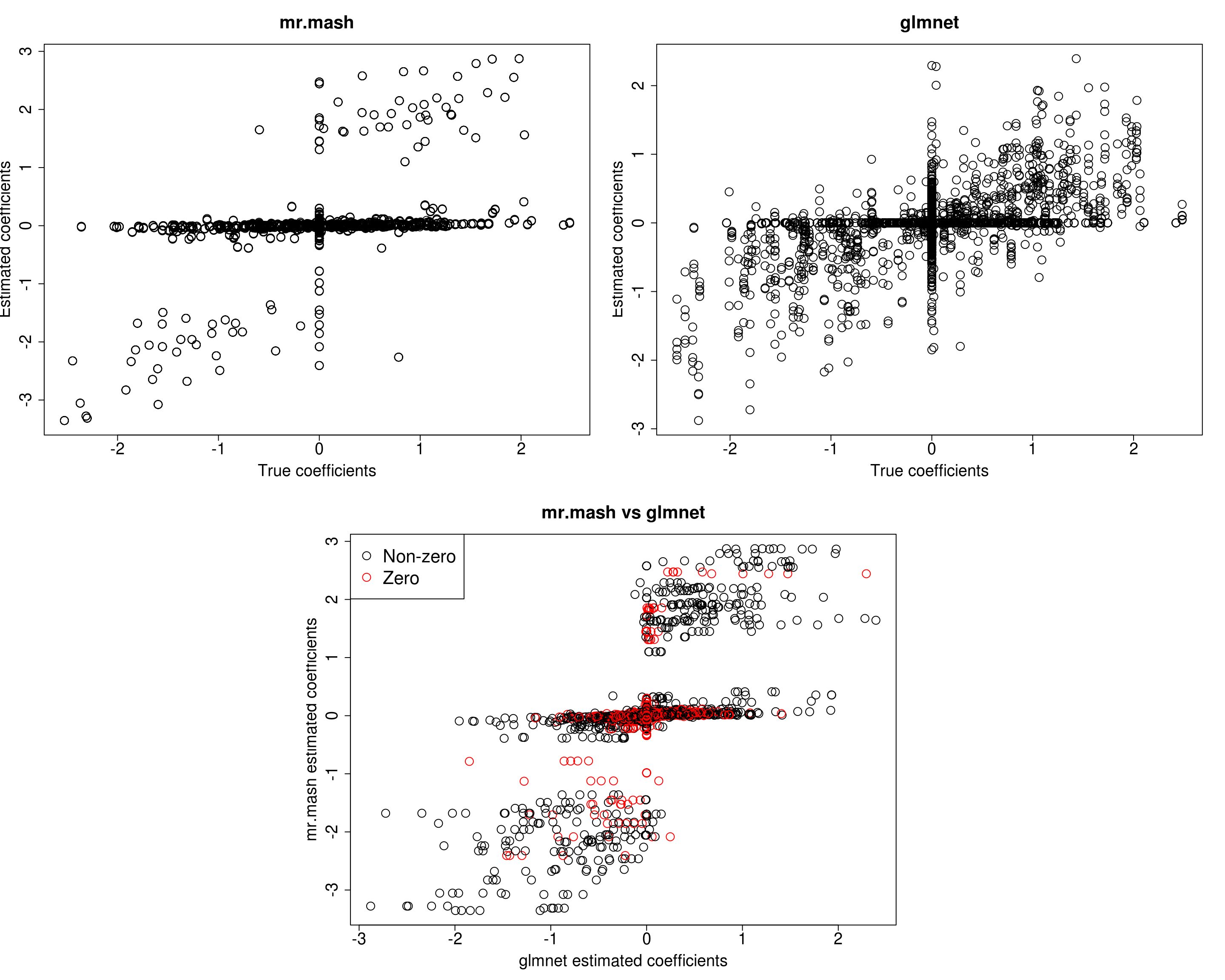
| Version | Author | Date |
|---|---|---|
| 5328c22 | fmorgante | 2020-06-02 |
print("Prediction performance with glmnet")[1] "Prediction performance with glmnet"compute_accuracy(Ytest, Yhat_test_glmnet)$bias
[1] 0.7973441 0.7171240 1.1201318 0.9992656 0.9375002
$r2
[1] 0.12560024 0.10044653 0.14357016 0.13204939 0.09516285
$mse
[1] 502.2840 531.2713 573.5326 575.3974 722.7162print("Prediction performance with mr.mash")[1] "Prediction performance with mr.mash"compute_accuracy(Ytest, Yhat_test_mrmash_diagV)$bias
[1] 0.4126154 0.3465257 0.5752667 0.5588387 0.5719653
$r2
[1] 0.08870657 0.06277994 0.14750399 0.14278998 0.12151611
$mse
[1] 628.5332 698.4433 623.4901 649.4620 762.7409print("True V (full data)")[1] "True V (full data)"out$V [,1] [,2] [,3] [,4] [,5]
[1,] 331.4137 0.0000 0.0000 0.0000 0.0000
[2,] 0.0000 331.4137 0.0000 0.0000 0.0000
[3,] 0.0000 0.0000 331.4137 0.0000 0.0000
[4,] 0.0000 0.0000 0.0000 331.4137 0.0000
[5,] 0.0000 0.0000 0.0000 0.0000 331.4137print("Estimated V (training data)")[1] "Estimated V (training data)"fit_mrmash_diagV$V Y1 Y2 Y3 Y4 Y5
Y1 397.6517 0.0000 0.0000 0.0000 0.0000
Y2 0.0000 340.6878 0.0000 0.0000 0.0000
Y3 0.0000 0.0000 335.3694 0.0000 0.0000
Y4 0.0000 0.0000 0.0000 337.8452 0.0000
Y5 0.0000 0.0000 0.0000 0.0000 319.6164Although the estimated residual covariance is much closer to the truth and now many coefficients are not overshrunk, prediction performance is still poor. Another possibility is that overshrinking of coefficients happens because the mixture weights are poorly initialized. Let’s now try to initialize the mixture weights to the truth.
###Fit mr.mash
w0 <- rep(0, length(S0))
w0[c(104, 111)] <- c(0.5, 0.5)
fit_mrmash_diagV_initw0 <- mr.mash(Xtrain, Ytrain, S0, w0=w0, tol=1e-2, convergence_criterion="ELBO", update_w0=TRUE,
                                   update_w0_method="EM", compute_ELBO=TRUE, standardize=TRUE, verbose=FALSE, update_V=TRUE,
                                   update_V_method="diagonal", mu1_init=Bhat_glmnet, w0_threshold=1e-8)
Processing the inputs... Done!
Fitting the optimization algorithm... Done!
Processing the outputs... Done!
mr.mash successfully executed in 0.3481156 minutes!Yhat_test_mrmash_diagV_initw0 <- predict(fit_mrmash_diagV_initw0, Xtest)layout(matrix(c(1, 1, 2, 2,
1, 1, 2, 2,
0, 3, 3, 0,
0, 3, 3, 0), 4, 4, byrow = TRUE))
###Plot estimated vs true coeffcients
##mr.mash
plot(out$B, fit_mrmash_diagV_initw0$mu1, main="mr.mash", xlab="True coefficients", ylab="Estimated coefficients",
cex=2, cex.lab=1.8, cex.main=2, cex.axis=1.8)
##glmnet
plot(out$B, Bhat_glmnet, main="glmnet", xlab="True coefficients", ylab="Estimated coefficients",
cex=2, cex.lab=1.8, cex.main=2, cex.axis=1.8)
###Plot mr.mash vs glmnet estimated coeffcients
colorz <- matrix("black", nrow=p, ncol=r)
zeros <- apply(out$B, 2, function(x) x==0)
for(i in 1:ncol(colorz)){
colorz[zeros[, i], i] <- "red"
}
plot(Bhat_glmnet, fit_mrmash_diagV_initw0$mu1, main="mr.mash vs glmnet",
xlab="glmnet estimated coefficients", ylab="mr.mash estimated coefficients",
col=colorz, cex=2, cex.lab=1.8, cex.main=2, cex.axis=1.8)
legend("topleft",
legend = c("Non-zero", "Zero"),
col = c("black", "red"),
pch = c(1, 1),
horiz = FALSE,
cex=2) 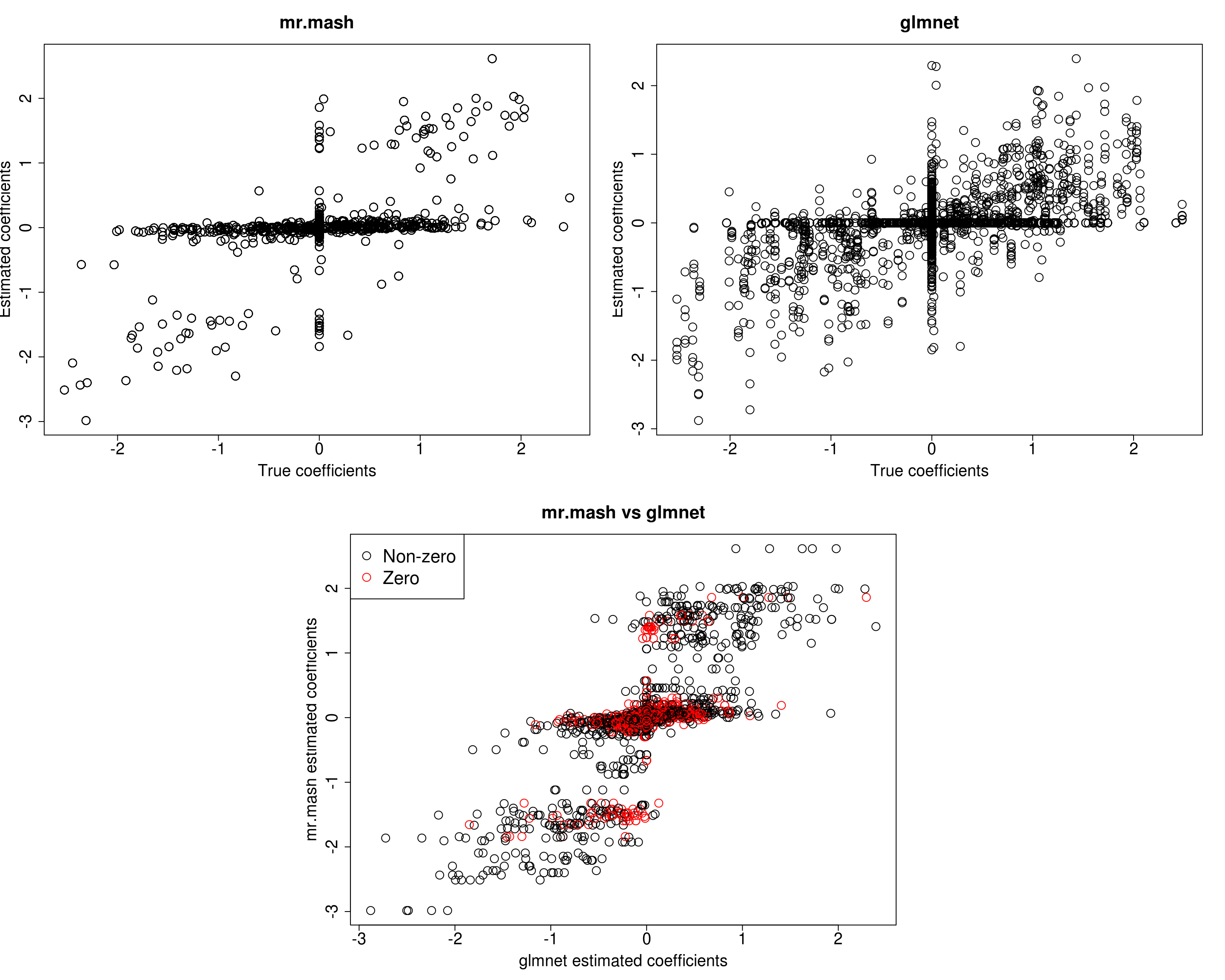
| Version | Author | Date |
|---|---|---|
| 5328c22 | fmorgante | 2020-06-02 |
print("Prediction performance with glmnet")[1] "Prediction performance with glmnet"compute_accuracy(Ytest, Yhat_test_glmnet)$bias
[1] 0.7973441 0.7171240 1.1201318 0.9992656 0.9375002
$r2
[1] 0.12560024 0.10044653 0.14357016 0.13204939 0.09516285
$mse
[1] 502.2840 531.2713 573.5326 575.3974 722.7162print("Prediction performance with mr.mash")[1] "Prediction performance with mr.mash"compute_accuracy(Ytest, Yhat_test_mrmash_diagV_initw0)$bias
[1] 0.6137635 0.6313922 0.7989912 0.8056523 0.6864326
$r2
[1] 0.1287113 0.1368245 0.1864412 0.1935577 0.1148231
$mse
[1] 525.1827 533.7511 549.6033 545.9291 725.6260print("True V (full data)")[1] "True V (full data)"out$V [,1] [,2] [,3] [,4] [,5]
[1,] 331.4137 0.0000 0.0000 0.0000 0.0000
[2,] 0.0000 331.4137 0.0000 0.0000 0.0000
[3,] 0.0000 0.0000 331.4137 0.0000 0.0000
[4,] 0.0000 0.0000 0.0000 331.4137 0.0000
[5,] 0.0000 0.0000 0.0000 0.0000 331.4137print("Estimated V (training data)")[1] "Estimated V (training data)"fit_mrmash_diagV_initw0$V Y1 Y2 Y3 Y4 Y5
Y1 407.9608 0.0000 0.0000 0.0000 0.0000
Y2 0.0000 346.9626 0.0000 0.0000 0.0000
Y3 0.0000 0.0000 349.2363 0.0000 0.0000
Y4 0.0000 0.0000 0.0000 345.4373 0.0000
Y5 0.0000 0.0000 0.0000 0.0000 328.7146Now, prediction performance is better. Next, let’s try to fix the mixture weights to the truth.
###Fit mr.mash
fit_mrmash_diagV_truew0 <- mr.mash(Xtrain, Ytrain, S0, w0=w0, tol=1e-2, convergence_criterion="ELBO", update_w0=FALSE,
                                    update_w0_method="EM", compute_ELBO=TRUE, standardize=TRUE, verbose=FALSE, update_V=TRUE,
                                    update_V_method="diagonal", mu1_init=Bhat_glmnet, w0_threshold=1e-8)
Processing the inputs... Done!
Fitting the optimization algorithm... Done!
Processing the outputs... Done!
mr.mash successfully executed in 0.7473614 minutes!Yhat_test_mrmash_diagV_truew0 <- predict(fit_mrmash_diagV_truew0, Xtest)layout(matrix(c(1, 1, 2, 2,
1, 1, 2, 2,
0, 3, 3, 0,
0, 3, 3, 0), 4, 4, byrow = TRUE))
###Plot estimated vs true coeffcients
##mr.mash
plot(out$B, fit_mrmash_diagV_truew0$mu1, main="mr.mash", xlab="True coefficients", ylab="Estimated coefficients",
cex=2, cex.lab=1.8, cex.main=2, cex.axis=1.8)
##glmnet
plot(out$B, Bhat_glmnet, main="glmnet", xlab="True coefficients", ylab="Estimated coefficients",
cex=2, cex.lab=1.8, cex.main=2, cex.axis=1.8)
###Plot mr.mash vs glmnet estimated coeffcients
colorz <- matrix("black", nrow=p, ncol=r)
zeros <- apply(out$B, 2, function(x) x==0)
for(i in 1:ncol(colorz)){
colorz[zeros[, i], i] <- "red"
}
plot(Bhat_glmnet, fit_mrmash_diagV_truew0$mu1, main="mr.mash vs glmnet",
xlab="glmnet estimated coefficients", ylab="mr.mash estimated coefficients",
col=colorz, cex=2, cex.lab=1.8, cex.main=2, cex.axis=1.8)
legend("topleft",
legend = c("Non-zero", "Zero"),
col = c("black", "red"),
pch = c(1, 1),
horiz = FALSE,
cex=2) 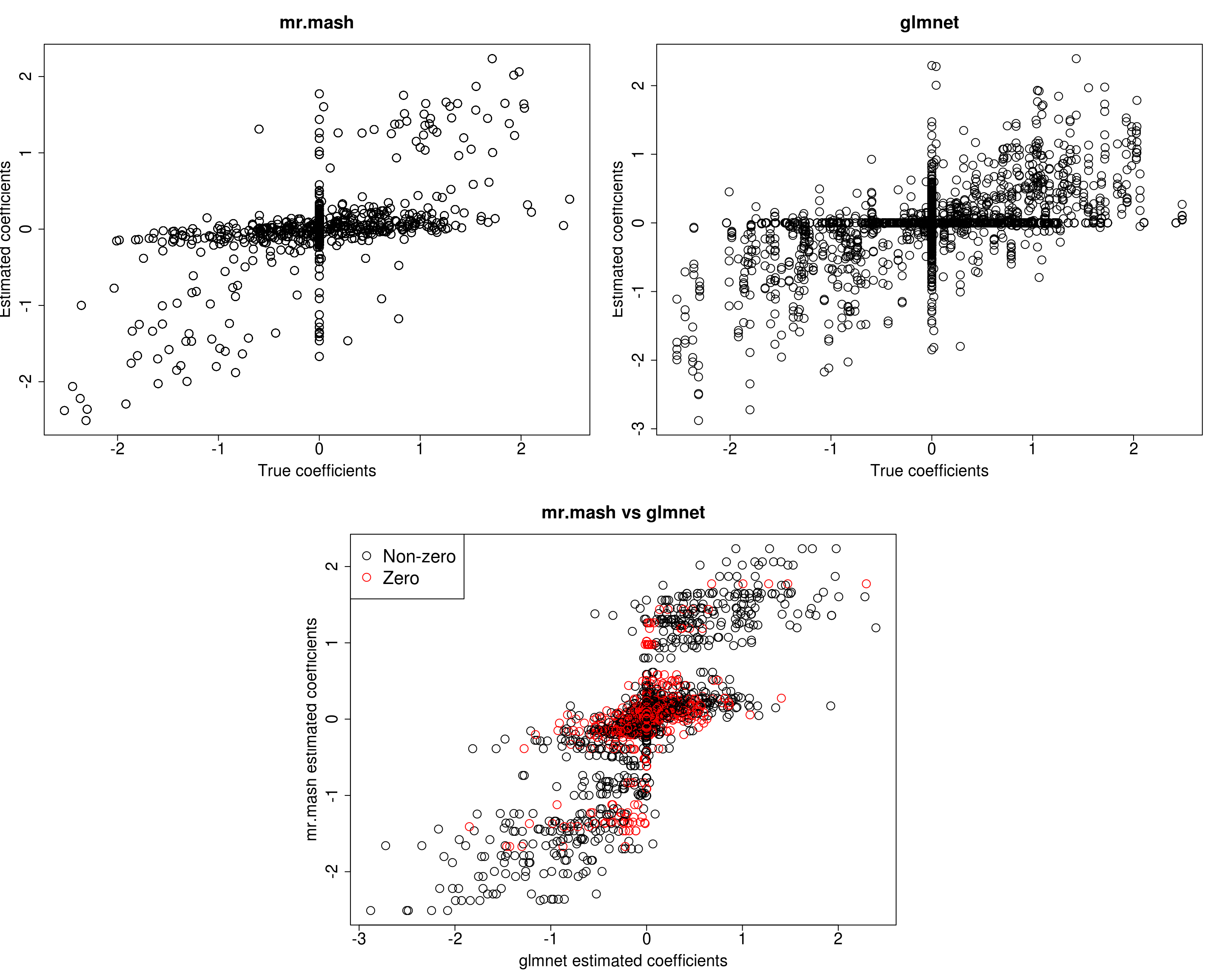
| Version | Author | Date |
|---|---|---|
| 5328c22 | fmorgante | 2020-06-02 |
print("Prediction performance with glmnet")[1] "Prediction performance with glmnet"compute_accuracy(Ytest, Yhat_test_glmnet)$bias
[1] 0.7973441 0.7171240 1.1201318 0.9992656 0.9375002
$r2
[1] 0.12560024 0.10044653 0.14357016 0.13204939 0.09516285
$mse
[1] 502.2840 531.2713 573.5326 575.3974 722.7162print("Prediction performance with mr.mash")[1] "Prediction performance with mr.mash"compute_accuracy(Ytest, Yhat_test_mrmash_diagV_truew0)$bias
[1] 0.7032514 0.7018678 0.9482747 0.9433495 0.8535756
$r2
[1] 0.1447663 0.1448465 0.2249874 0.2273485 0.1521071
$mse
[1] 501.5878 516.7773 516.6486 516.4104 680.2251print("True V (full data)")[1] "True V (full data)"out$V [,1] [,2] [,3] [,4] [,5]
[1,] 331.4137 0.0000 0.0000 0.0000 0.0000
[2,] 0.0000 331.4137 0.0000 0.0000 0.0000
[3,] 0.0000 0.0000 331.4137 0.0000 0.0000
[4,] 0.0000 0.0000 0.0000 331.4137 0.0000
[5,] 0.0000 0.0000 0.0000 0.0000 331.4137print("Estimated V (training data)")[1] "Estimated V (training data)"fit_mrmash_diagV_truew0$V Y1 Y2 Y3 Y4 Y5
Y1 419.9455 0.0000 0.0000 0.000 0.0000
Y2 0.0000 349.1219 0.0000 0.000 0.0000
Y3 0.0000 0.0000 355.0746 0.000 0.0000
Y4 0.0000 0.0000 0.0000 355.097 0.0000
Y5 0.0000 0.0000 0.0000 0.000 333.5331Prediction accuracy is now good and better than group-lasso. Finally, let’s fix both the residual covariance and mixture weights to the truth.
###Fit mr.mash
fit_mrmash_trueV_truew0 <- mr.mash(Xtrain, Ytrain, S0, w0=w0, tol=1e-2, convergence_criterion="ELBO", update_w0=FALSE,
                                    update_w0_method="EM", compute_ELBO=TRUE, standardize=TRUE, verbose=FALSE, update_V=FALSE,
                                    update_V_method="diagonal", mu1_init=Bhat_glmnet, w0_threshold=1e-8, V=out$V)
Processing the inputs... Done!
Fitting the optimization algorithm... Done!
Processing the outputs... Done!
mr.mash successfully executed in 0.7254679 minutes!Yhat_test_mrmash_trueV_truew0 <- predict(fit_mrmash_trueV_truew0, Xtest)layout(matrix(c(1, 1, 2, 2,
1, 1, 2, 2,
0, 3, 3, 0,
0, 3, 3, 0), 4, 4, byrow = TRUE))
###Plot estimated vs true coeffcients
##mr.mash
plot(out$B, fit_mrmash_trueV_truew0$mu1, main="mr.mash", xlab="True coefficients", ylab="Estimated coefficients",
cex=2, cex.lab=1.8, cex.main=2, cex.axis=1.8)
##glmnet
plot(out$B, Bhat_glmnet, main="glmnet", xlab="True coefficients", ylab="Estimated coefficients",
cex=2, cex.lab=1.8, cex.main=2, cex.axis=1.8)
###Plot mr.mash vs glmnet estimated coeffcients
colorz <- matrix("black", nrow=p, ncol=r)
zeros <- apply(out$B, 2, function(x) x==0)
for(i in 1:ncol(colorz)){
colorz[zeros[, i], i] <- "red"
}
plot(Bhat_glmnet, fit_mrmash_trueV_truew0$mu1, main="mr.mash vs glmnet",
xlab="glmnet estimated coefficients", ylab="mr.mash estimated coefficients",
col=colorz, cex=2, cex.lab=1.8, cex.main=2, cex.axis=1.8)
legend("topleft",
legend = c("Non-zero", "Zero"),
col = c("black", "red"),
pch = c(1, 1),
horiz = FALSE,
cex=2) 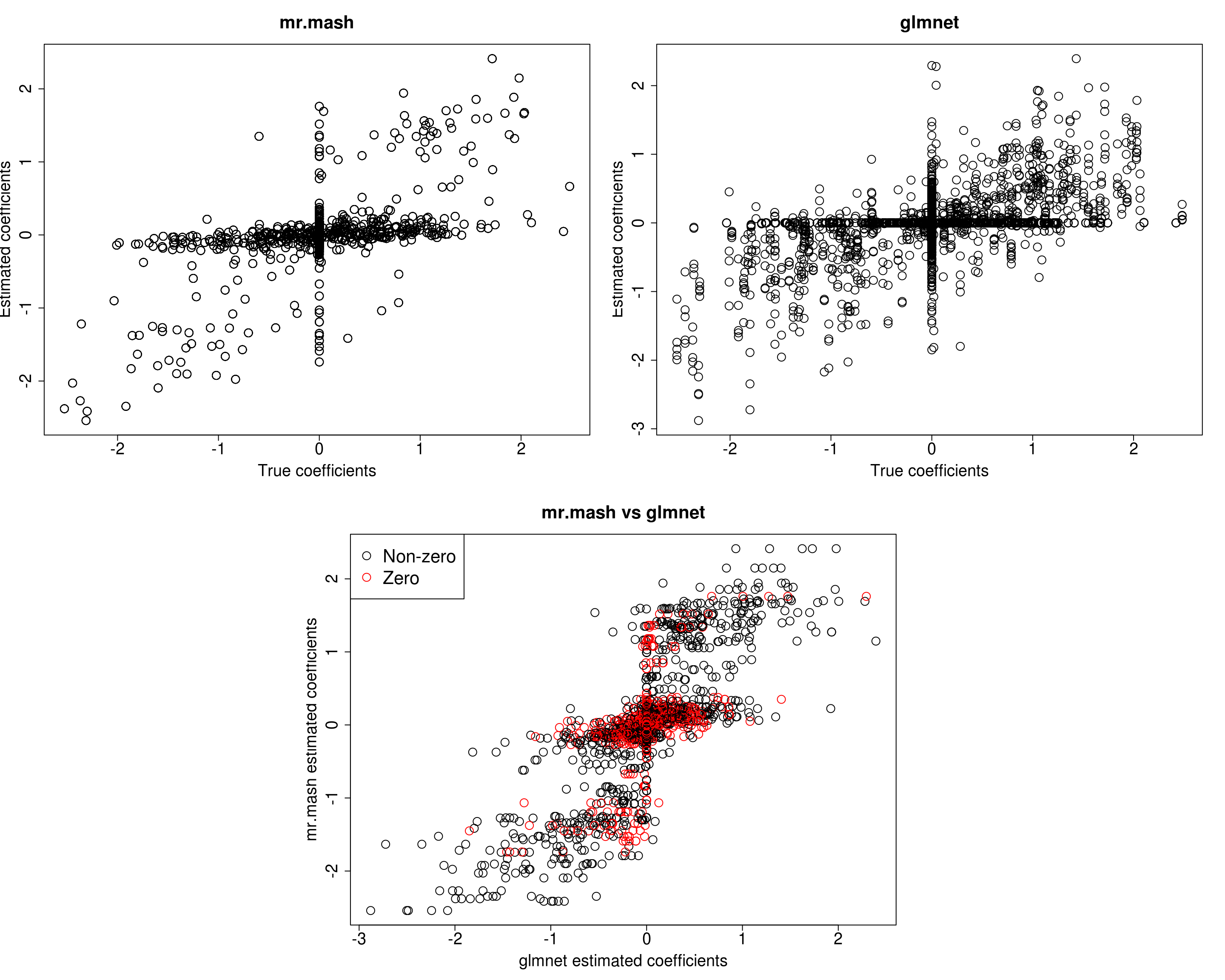
| Version | Author | Date |
|---|---|---|
| 5328c22 | fmorgante | 2020-06-02 |
print("Prediction performance with glmnet")[1] "Prediction performance with glmnet"compute_accuracy(Ytest, Yhat_test_glmnet)$bias
[1] 0.7973441 0.7171240 1.1201318 0.9992656 0.9375002
$r2
[1] 0.12560024 0.10044653 0.14357016 0.13204939 0.09516285
$mse
[1] 502.2840 531.2713 573.5326 575.3974 722.7162print("Prediction performance with mr.mash")[1] "Prediction performance with mr.mash"compute_accuracy(Ytest, Yhat_test_mrmash_trueV_truew0)$bias
[1] 0.7029293 0.6891626 0.9544747 0.9387136 0.8622740
$r2
[1] 0.1516346 0.1464096 0.2389721 0.2360162 0.1627364
$mse
[1] 498.3975 517.7781 507.2839 510.7310 671.4638Not surprisingly we now achieve the best accuracy of all models.
However, looking at ELBO for all the models fitted so far reveals something interesting. The models that provide the best prediction performance in the test set are those with smaller ELBO, and viceversa. My intuition is that the largest ELBO is due to those models having more free parameters (since the include updating the weights and V with no structure imposed).
print(paste("Update w0, update V:", fit_mrmash$ELBO))[1] "Update w0, update V: -10789.3132448488"print(paste("Update w0, fix V to the truth:", fit_mrmash_fixV$ELBO))[1] "Update w0, fix V to the truth: -10858.0496418998"print(paste("Update w0, update V initializing it to the truth:", fit_mrmash_initV$ELBO))[1] "Update w0, update V initializing it to the truth: -10789.303405305"print(paste("Update w0, update V imposing a diagonal structure:", fit_mrmash_diagV$ELBO))[1] "Update w0, update V imposing a diagonal structure: -10855.1638789792"print(paste("Update w0 initializing them to the truth, update V imposing a diagonal structure:", fit_mrmash_diagV_initw0$ELBO))[1] "Update w0 initializing them to the truth, update V imposing a diagonal structure: -10869.1875885718"print(paste("Fix w0 to the truth, update V imposing a diagonal structure:", fit_mrmash_diagV_truew0$ELBO))[1] "Fix w0 to the truth, update V imposing a diagonal structure: -10936.6653594846"print(paste("Fix w0 and V to the truth:", fit_mrmash_trueV_truew0$ELBO))[1] "Fix w0 and V to the truth: -10942.8402970471"Sparser scenario
For comparison let’s try to repeat the analysis above (updating V) on a sparser scenario, i.e., p_causal=50.
###Set parameters
n <- 600
p <- 1000
p_causal <- 50
r <- 5
r_causal <- r
pve <- 0.5
B_cor <- 1
X_cor <- 0
V_cor <- 0

###Simulate V, B, X and Y
out50 <- mr.mash.alpha:::simulate_mr_mash_data(n, p, p_causal, r, r_causal=r, intercepts = rep(1, r),
                                             pve=pve, B_cor=B_cor, B_scale=0.8, X_cor=X_cor, X_scale=0.8, V_cor=V_cor)

colnames(out50$Y) <- paste0("Y", seq(1, r))
rownames(out50$Y) <- paste0("N", seq(1, n))
colnames(out50$X) <- paste0("X", seq(1, p))
rownames(out50$X) <- paste0("N", seq(1, n))

###Split the data in training and test sets
test_set50 <- sort(sample(x=c(1:n), size=round(n*0.2), replace=FALSE))
Ytrain50 <- out50$Y[-test_set50, ]
Xtrain50 <- out50$X[-test_set50, ]
Ytest50 <- out50$Y[test_set50, ]
Xtest50 <- out50$X[test_set50, ]

###Fit group-lasso
cvfit_glmnet50 <- cv.glmnet(x=Xtrain50, y=Ytrain50, family="mgaussian", alpha=1)
coeff_glmnet50 <- coef(cvfit_glmnet50, s="lambda.min")
Bhat_glmnet50 <- matrix(as.numeric(NA), nrow=p, ncol=r)
ahat_glmnet50 <- vector("numeric", r)
for(i in 1:length(coeff_glmnet50)){
  Bhat_glmnet50[, i] <- as.vector(coeff_glmnet50[[i]])[-1]
  ahat_glmnet50[i] <- as.vector(coeff_glmnet50[[i]])[1]
}
Yhat_test_glmnet50 <- drop(predict(cvfit_glmnet50, newx=Xtest50, s="lambda.min"))

###Fit mr.mash
fit_mrmash50 <- mr.mash(Xtrain50, Ytrain50, S0, tol=1e-2, convergence_criterion="ELBO", update_w0=TRUE,
                     update_w0_method="EM", compute_ELBO=TRUE, standardize=TRUE, verbose=FALSE, update_V=TRUE,
                     mu1_init = Bhat_glmnet50, w0_threshold=1e-8)
Processing the inputs... Done!
Fitting the optimization algorithm... Done!
Processing the outputs... Done!
mr.mash successfully executed in 0.9007726 minutes!Yhat_test_mrmash50 <- predict(fit_mrmash50, Xtest50)layout(matrix(c(1, 1, 2, 2,
1, 1, 2, 2,
0, 3, 3, 0,
0, 3, 3, 0), 4, 4, byrow = TRUE))
###Plot estimated vs true coeffcients
##mr.mash
plot(out50$B, fit_mrmash50$mu1, main="mr.mash", xlab="True coefficients", ylab="Estimated coefficients",
cex=2, cex.lab=1.8, cex.main=2, cex.axis=1.8)
##glmnet
plot(out50$B, Bhat_glmnet50, main="glmnet", xlab="True coefficients", ylab="Estimated coefficients",
cex=2, cex.lab=1.8, cex.main=2, cex.axis=1.8)
###Plot mr.mash vs glmnet estimated coeffcients
colorz <- matrix("black", nrow=p, ncol=r)
zeros <- apply(out50$B, 2, function(x) x==0)
for(i in 1:ncol(colorz)){
colorz[zeros[, i], i] <- "red"
}
plot(Bhat_glmnet50, fit_mrmash50$mu1, main="mr.mash vs glmnet",
xlab="glmnet estimated coefficients", ylab="mr.mash estimated coefficients",
col=colorz, cex=2, cex.lab=1.8, cex.main=2, cex.axis=1.8)
legend("topleft",
legend = c("Non-zero", "Zero"),
col = c("black", "red"),
pch = c(1, 1),
horiz = FALSE,
cex=2) 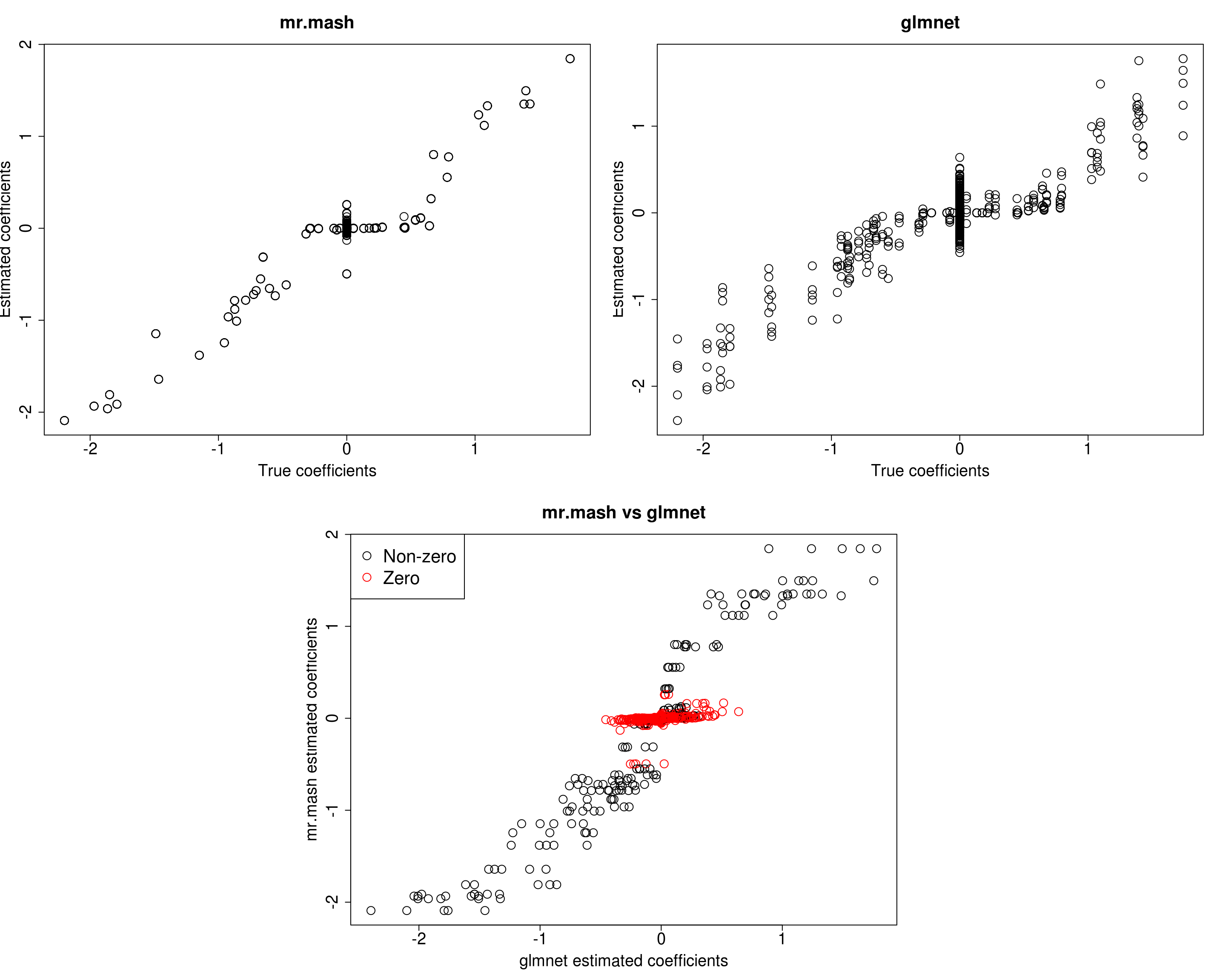
| Version | Author | Date |
|---|---|---|
| 42ec51c | fmorgante | 2020-06-01 |
print("Prediction performance with glmnet")[1] "Prediction performance with glmnet"compute_accuracy(Ytest50, Yhat_test_glmnet50)$bias
[1] 1.1055781 1.2342390 0.8929952 1.2093933 1.1997154
$r2
[1] 0.3720343 0.4451268 0.2709590 0.3909355 0.4424055
$mse
[1] 50.11301 49.98023 54.17894 53.96508 46.36995print("Prediction performance with mr.mash")[1] "Prediction performance with mr.mash"compute_accuracy(Ytest50, Yhat_test_mrmash50)$bias
[1] 0.9295387 1.1205934 0.8382439 0.9741666 1.0034935
$r2
[1] 0.4227190 0.5544520 0.3641726 0.4142314 0.4747928
$mse
[1] 46.04314 39.62819 48.00426 51.00798 42.98684print("True V (full data)")[1] "True V (full data)"out50$V [,1] [,2] [,3] [,4] [,5]
[1,] 43.262 0.000 0.000 0.000 0.000
[2,] 0.000 43.262 0.000 0.000 0.000
[3,] 0.000 0.000 43.262 0.000 0.000
[4,] 0.000 0.000 0.000 43.262 0.000
[5,] 0.000 0.000 0.000 0.000 43.262print("Estimated V (training data)")[1] "Estimated V (training data)"fit_mrmash50$V Y1 Y2 Y3 Y4 Y5
Y1 37.0783688 2.693322 2.7229456 3.426152 -0.6935028
Y2 2.6933223 42.243137 2.0293575 1.966294 2.6486737
Y3 2.7229456 2.029357 37.9331012 -2.456907 -0.2269764
Y4 3.4261520 1.966294 -2.4569072 42.752140 -3.0717702
Y5 -0.6935028 2.648674 -0.2269764 -3.071770 43.5576891The results of this simulation look very good in terms of prediction performance, estimation of the coefficients, and estimation of the residual covariance.
Dense scenario (fewer variables)
Just as an additional test let’s now try to maintain the same signal-to-noise ratio as the first simulation but with fewer total variables, i.e., p=500 and p_causal=250.
###Set parameters
n <- 600
p <- 500
p_causal <- 250
r <- 5
r_causal <- r
pve <- 0.5
B_cor <- 1
X_cor <- 0
V_cor <- 0

###Simulate V, B, X and Y
out500 <- mr.mash.alpha:::simulate_mr_mash_data(n, p, p_causal, r, r_causal=r, intercepts = rep(1, r),
                                             pve=pve, B_cor=B_cor, B_scale=0.8, X_cor=X_cor, X_scale=0.8, V_cor=V_cor)

colnames(out500$Y) <- paste0("Y", seq(1, r))
rownames(out500$Y) <- paste0("N", seq(1, n))
colnames(out500$X) <- paste0("X", seq(1, p))
rownames(out500$X) <- paste0("N", seq(1, n))

###Split the data in training and test sets
test_set500 <- sort(sample(x=c(1:n), size=round(n*0.2), replace=FALSE))
Ytrain500 <- out500$Y[-test_set500, ]
Xtrain500 <- out500$X[-test_set500, ]
Ytest500 <- out500$Y[test_set500, ]
Xtest500 <- out500$X[test_set500, ]

###Fit group-lasso
cvfit_glmnet500 <- cv.glmnet(x=Xtrain500, y=Ytrain500, family="mgaussian", alpha=1)
coeff_glmnet500 <- coef(cvfit_glmnet500, s="lambda.min")
Bhat_glmnet500 <- matrix(as.numeric(NA), nrow=p, ncol=r)
ahat_glmnet500 <- vector("numeric", r)
for(i in 1:length(coeff_glmnet500)){
  Bhat_glmnet500[, i] <- as.vector(coeff_glmnet500[[i]])[-1]
  ahat_glmnet500[i] <- as.vector(coeff_glmnet500[[i]])[1]
}
Yhat_test_glmnet500 <- drop(predict(cvfit_glmnet500, newx=Xtest500, s="lambda.min"))

###Fit mr.mash
fit_mrmash500 <- mr.mash(Xtrain500, Ytrain500, S0, tol=1e-2, convergence_criterion="ELBO", update_w0=TRUE,
                     update_w0_method="EM", compute_ELBO=TRUE, standardize=TRUE, verbose=FALSE, update_V=TRUE,
                     mu1_init = Bhat_glmnet500, w0_threshold=1e-8)
Processing the inputs... Done!
Fitting the optimization algorithm... Done!
Processing the outputs... Done!
mr.mash successfully executed in 1.153135 minutes!Yhat_test_mrmash500 <- predict(fit_mrmash500, Xtest500)layout(matrix(c(1, 1, 2, 2,
1, 1, 2, 2,
0, 3, 3, 0,
0, 3, 3, 0), 4, 4, byrow = TRUE))
###Plot estimated vs true coeffcients
##mr.mash
plot(out500$B, fit_mrmash500$mu1, main="mr.mash", xlab="True coefficients", ylab="Estimated coefficients",
cex=2, cex.lab=1.8, cex.main=2, cex.axis=1.8)
##glmnet
plot(out500$B, Bhat_glmnet500, main="glmnet", xlab="True coefficients", ylab="Estimated coefficients",
cex=2, cex.lab=1.8, cex.main=2, cex.axis=1.8)
###Plot mr.mash vs glmnet estimated coeffcients
colorz <- matrix("black", nrow=p, ncol=r)
zeros <- apply(out500$B, 2, function(x) x==0)
for(i in 1:ncol(colorz)){
colorz[zeros[, i], i] <- "red"
}
plot(Bhat_glmnet500, fit_mrmash500$mu1, main="mr.mash vs glmnet",
xlab="glmnet estimated coefficients", ylab="mr.mash estimated coefficients",
col=colorz, cex=2, cex.lab=1.8, cex.main=2, cex.axis=1.8)
legend("topleft",
legend = c("Non-zero", "Zero"),
col = c("black", "red"),
pch = c(1, 1),
horiz = FALSE,
cex=2) 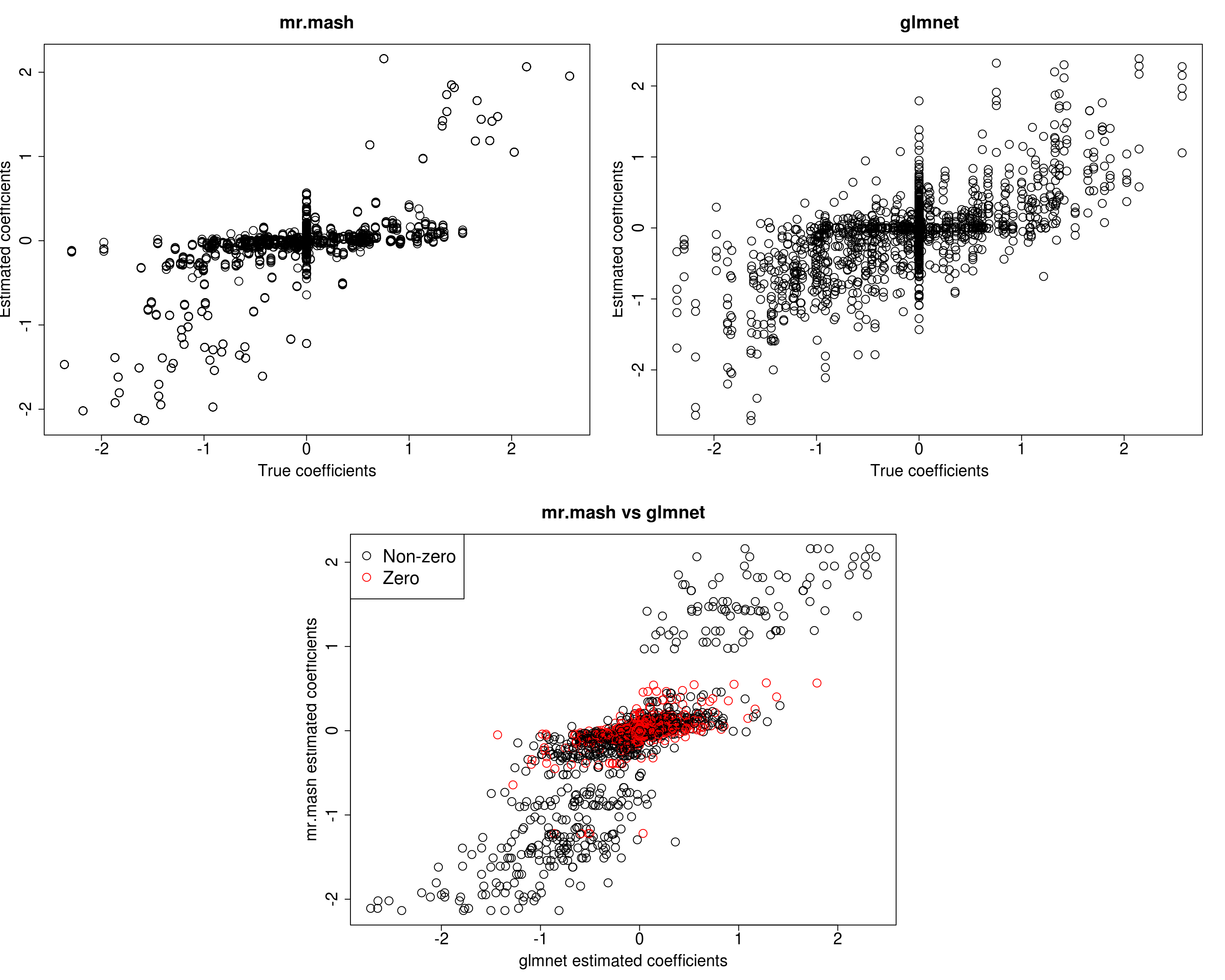
| Version | Author | Date |
|---|---|---|
| 42ec51c | fmorgante | 2020-06-01 |
print("Prediction performance with glmnet")[1] "Prediction performance with glmnet"compute_accuracy(Ytest500, Yhat_test_glmnet500)$bias
[1] 0.7460558 0.8379627 0.8827708 1.0150154 0.8988217
$r2
[1] 0.1566151 0.1754140 0.2246133 0.2126951 0.2354353
$mse
[1] 262.5938 307.5913 280.3553 259.2769 265.2623print("Prediction performance with mr.mash")[1] "Prediction performance with mr.mash"compute_accuracy(Ytest500, Yhat_test_mrmash500)$bias
[1] 0.8007963 1.0543346 0.9437460 0.9812104 1.0269983
$r2
[1] 0.1917870 0.2740736 0.2402338 0.2626540 0.2816563
$mse
[1] 249.0113 269.0810 268.4814 242.8198 247.6815print("True V (full data)")[1] "True V (full data)"out500$V [,1] [,2] [,3] [,4] [,5]
[1,] 168.3364 0.0000 0.0000 0.0000 0.0000
[2,] 0.0000 168.3364 0.0000 0.0000 0.0000
[3,] 0.0000 0.0000 168.3364 0.0000 0.0000
[4,] 0.0000 0.0000 0.0000 168.3364 0.0000
[5,] 0.0000 0.0000 0.0000 0.0000 168.3364print("Estimated V (training data)")[1] "Estimated V (training data)"fit_mrmash500$V Y1 Y2 Y3 Y4 Y5
Y1 190.385218 4.826421 31.00999 22.18042 5.743413
Y2 4.826421 181.999035 16.65374 8.40475 9.590063
Y3 31.009989 16.653736 198.77957 39.23005 35.494926
Y4 22.180421 8.404750 39.23005 209.04480 25.167324
Y5 5.743413 9.590063 35.49493 25.16732 194.837000In this last simulation, we can see that mr.mash performs pretty well, even in a denser scenario with fewer variables.
sessionInfo()R version 3.5.1 (2018-07-02)
Platform: x86_64-pc-linux-gnu (64-bit)
Running under: Scientific Linux 7.4 (Nitrogen)
Matrix products: default
BLAS/LAPACK: /software/openblas-0.2.19-el7-x86_64/lib/libopenblas_haswellp-r0.2.19.so
locale:
[1] LC_CTYPE=en_US.UTF-8 LC_NUMERIC=C
[3] LC_TIME=en_US.UTF-8 LC_COLLATE=en_US.UTF-8
[5] LC_MONETARY=en_US.UTF-8 LC_MESSAGES=en_US.UTF-8
[7] LC_PAPER=en_US.UTF-8 LC_NAME=C
[9] LC_ADDRESS=C LC_TELEPHONE=C
[11] LC_MEASUREMENT=en_US.UTF-8 LC_IDENTIFICATION=C
attached base packages:
[1] stats graphics grDevices utils datasets methods base
other attached packages:
[1] glmnet_2.0-16 foreach_1.4.4 Matrix_1.2-15
[4] mr.mash.alpha_0.1-76
loaded via a namespace (and not attached):
[1] MBSP_1.0 Rcpp_1.0.4.6 compiler_3.5.1
[4] later_0.7.5 git2r_0.26.1 workflowr_1.6.1
[7] iterators_1.0.10 tools_3.5.1 digest_0.6.25
[10] evaluate_0.12 lattice_0.20-38 GIGrvg_0.5
[13] yaml_2.2.1 SparseM_1.77 mvtnorm_1.0-12
[16] coda_0.19-3 stringr_1.4.0 knitr_1.20
[19] fs_1.3.1 MatrixModels_0.4-1 rprojroot_1.3-2
[22] grid_3.5.1 glue_1.4.0 R6_2.4.1
[25] rmarkdown_1.10 mixsqp_0.3-43 irlba_2.3.3
[28] magrittr_1.5 whisker_0.3-2 codetools_0.2-15
[31] backports_1.1.5 promises_1.0.1 htmltools_0.3.6
[34] matrixStats_0.55.0 mcmc_0.9-6 MASS_7.3-51.1
[37] httpuv_1.4.5 quantreg_5.36 stringi_1.4.3
[40] MCMCpack_1.4-4