Last updated: 2022-01-16

Checks: 7 0

Knit directory: false.alarm/

This reproducible R Markdown analysis was created with workflowr (version 1.7.0). The Checks tab describes the reproducibility checks that were applied when the results were created. The Past versions tab lists the development history.

R Markdown file: up-to-date

Great! Since the R Markdown file has been committed to the Git repository, you know the exact version of the code that produced these results.

Environment: empty

Great job! The global environment was empty. Objects defined in the global environment can affect the analysis in your R Markdown file in unknown ways. For reproduciblity it’s best to always run the code in an empty environment.

Seed: set.seed(20201020)

The command set.seed(20201020) was run prior to running the code in the R Markdown file. Setting a seed ensures that any results that rely on randomness, e.g. subsampling or permutations, are reproducible.

Session information: recorded

Great job! Recording the operating system, R version, and package versions is critical for reproducibility.

Cache: none

Nice! There were no cached chunks for this analysis, so you can be confident that you successfully produced the results during this run.

File paths: relative

Great job! Using relative paths to the files within your workflowr project makes it easier to run your code on other machines.

Repository version: afebf46

Great! You are using Git for version control. Tracking code development and connecting the code version to the results is critical for reproducibility.

The results in this page were generated with repository version afebf46. See the Past versions tab to see a history of the changes made to the R Markdown and HTML files.

Note that you need to be careful to ensure that all relevant files for the analysis have been committed to Git prior to generating the results (you can use wflow_publish or wflow_git_commit). workflowr only checks the R Markdown file, but you know if there are other scripts or data files that it depends on. Below is the status of the Git repository when the results were generated:


Ignored files:
    Ignored:    .Renviron
    Ignored:    .Rhistory
    Ignored:    .Rproj.user/
    Ignored:    .devcontainer/exts/
    Ignored:    .history
    Ignored:    .httr-oauth
    Ignored:    R/RcppExports.R
    Ignored:    _classifier/.gittargets
    Ignored:    _classifier/meta/process
    Ignored:    _classifier/meta/progress
    Ignored:    _classifier/objects/
    Ignored:    _classifier/user/
    Ignored:    _targets/.gitattributes
    Ignored:    _targets/.gittargets
    Ignored:    _targets/meta/process
    Ignored:    _targets/meta/progress
    Ignored:    _targets/objects/
    Ignored:    _targets/user/
    Ignored:    analysis/blog_cache/
    Ignored:    dev/
    Ignored:    inst/extdata/
    Ignored:    output/images/
    Ignored:    papers/aime2021/aime2021.md
    Ignored:    protocol/SecondReport.pdf
    Ignored:    protocol/SecondReport_cache/
    Ignored:    protocol/SecondReport_files/
    Ignored:    renv/library/
    Ignored:    renv/python/
    Ignored:    renv/staging/
    Ignored:    src/RcppExports.cpp
    Ignored:    src/RcppExports.o
    Ignored:    src/contrast.o
    Ignored:    src/false.alarm.so
    Ignored:    src/fft.o
    Ignored:    src/mass.o
    Ignored:    src/math.o
    Ignored:    src/mpx.o
    Ignored:    src/scrimp.o
    Ignored:    src/stamp.o
    Ignored:    src/stomp.o
    Ignored:    src/windowfunc.o
    Ignored:    tests/testthat/_snaps/
    Ignored:    tmp/

Note that any generated files, e.g. HTML, png, CSS, etc., are not included in this status report because it is ok for generated content to have uncommitted changes.

These are the previous versions of the repository in which changes were made to the R Markdown (analysis/report.Rmd) and HTML (docs/report.html) files. If you’ve configured a remote Git repository (see ?wflow_git_remote), click on the hyperlinks in the table below to view the files as they were in that past version.

File	Version	Author	Date	Message
Rmd	571ac34	Francisco Bischoff	2022-01-15	premerge
Rmd	dc34ece	Francisco Bischoff	2022-01-10	k_shapelets
html	95ae431	Francisco Bischoff	2022-01-05	blogdog
html	7278108	Francisco Bischoff	2021-12-21	update dataset on zenodo
Rmd	1ef8e75	Francisco Bischoff	2021-10-14	freeze for presentation
html	ca1941e	GitHub Actions	2021-10-12	Build site.
Rmd	6b03f43	Francisco Bischoff	2021-10-11	Squashed commit of the following:
html	c19ec01	Francisco Bischoff	2021-08-17	Build site.
html	a5ec160	Francisco Bischoff	2021-08-17	Build site.
html	b51dba2	GitHub Actions	2021-08-17	Build site.
Rmd	c88cbd5	Francisco Bischoff	2021-08-17	targets workflowr
html	c88cbd5	Francisco Bischoff	2021-08-17	targets workflowr
html	e7e5d48	GitHub Actions	2021-07-15	Build site.
Rmd	1473a05	Francisco Bischoff	2021-07-15	report
html	1473a05	Francisco Bischoff	2021-07-15	report
Rmd	7436fbe	Francisco Bischoff	2021-07-11	stage cpp code
html	7436fbe	Francisco Bischoff	2021-07-11	stage cpp code
html	52e7f0b	GitHub Actions	2021-03-24	Build site.
Rmd	7c3cc31	Francisco Bischoff	2021-03-23	Targets
html	7c3cc31	Francisco Bischoff	2021-03-23	Targets

1 Current Work Status

1.1 Principles

This research is being conducted using the Research Compendium principles¹:

Stick with the convention of your peers;
Keep data, methods, and output separated;
Specify your computational environment as clearly as you can.

Data management follows the FAIR principle (findable, accessible, interoperable, reusable)². Concerning these principles, the dataset was converted from Matlab’s format to CSV format, allowing more interoperability. Additionally, all the project, including the dataset, is in conformity with the Codemeta Project³.

1.2 The data

The current dataset used is the CinC/Physionet Challenge 2015 public dataset, modified to include only the actual data and the header files in order to be read by the pipeline and is hosted by Zenodo⁴ under the same license as Physionet.

The dataset is composed of 750 patients with at least five minutes records. All signals have been resampled (using anti-alias filters) to 12 bit, 250 Hz and have had FIR band-pass (0.05 to 40Hz) and mains notch filters applied to remove noise. Pacemaker and other artifacts are still present on the ECG⁵. Furthermore, this dataset contains at least two ECG derivations and one or more variables like arterial blood pressure, photoplethysmograph readings, and respiration movements.

The event we seek to improve is the detection of a life-threatening arrhythmia as defined by Physionet in Table 1.

Table 1 - Definition of the five alarm types used in CinC/Physionet Challenge 2015 challenge.
Alarm	Definition
Asystole	No QRS for at least 4 seconds
Extreme Bradycardia	Heart rate lower than 40 bpm for 5 consecutive beats
Extreme Tachycardia	Heart rate higher than 140 bpm for 17 consecutive beats
Ventricular Tachycardia	5 or more ventricular beats with heart rate higher than 100 bpm
Ventricular Flutter/Fibrillation	Fibrillatory, flutter, or oscillatory waveform for at least 4 seconds

The fifth minute is precisely where the alarm has been triggered on the original recording set. To meet the ANSI/AAMI EC13 Cardiac Monitor Standards⁶, the onset of the event is within 10 seconds of the alarm (i.e., between 4:50 and 5:00 of the record). That doesn’t mean that there are no other arrhythmias before, but those were not labeled.

1.3 Workflow

All steps of the process are being managed using the R package targets⁷ from data extraction to the final report, as shown in Fig. 1.

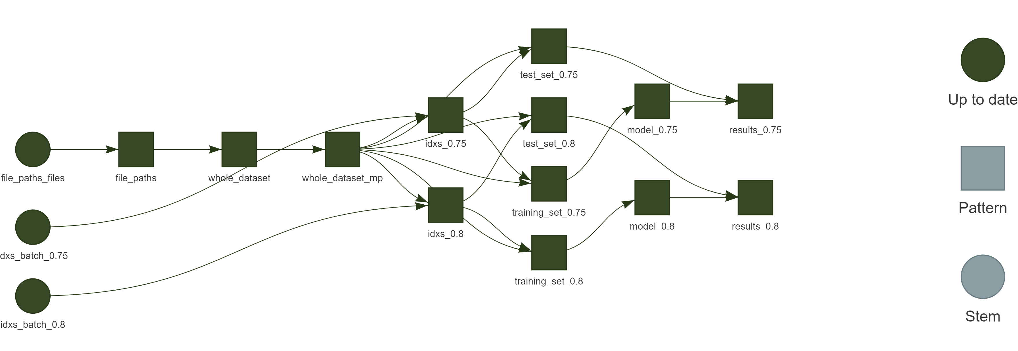
Figure 1 - Reproducible research workflow using targets.

Version	Author	Date
1473a05	Francisco Bischoff	2021-07-15

The report is available on the main webpage⁸, allowing inspection of previous versions managed by the R package workflowr⁹, as shown in Fig. 2.

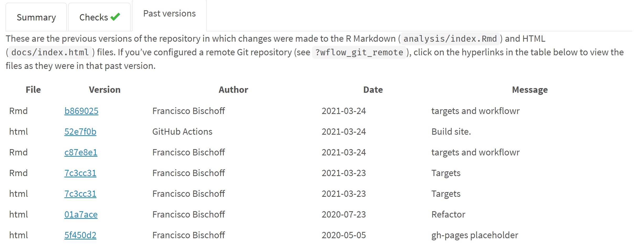
Figure 2 - Reproducible reports using workflowr.

Version	Author	Date
1473a05	Francisco Bischoff	2021-07-15

1.4 Work in Progress

1.4.1 Project start

The project started with a literature survey on the databases Scopus, Pubmed, Web of Science, and Google Scholar with the following query (the syntax was adapted for each database):

TITLE-ABS-KEY ( algorithm OR ‘point of care’ OR ‘signal processing’ OR ‘computer assisted’ OR ‘support vector machine’ OR ‘decision support system’ OR ’neural network’ OR ‘automatic interpretation’ OR ‘machine learning’) AND TITLE-ABS-KEY ( electrocardiography OR cardiography OR ‘electrocardiographic tracing’ OR ecg OR electrocardiogram OR cardiogram ) AND TITLE-ABS-KEY ( ‘Intensive care unit’ OR ‘cardiologic care unit’ OR ‘intensive care center’ OR ‘cardiologic care center’ )

The inclusion and exclusion criteria were defined as in Table 2.

Table 2 - Literature review criteria.
Inclusion criteria	Exclusion criteria
ECG automatic interpretation	Manual interpretation
ECG anomaly detection	Publication older than ten years
ECG context change detection	Do not attempt to identify life-threatening arrhythmias, namely asystole, extreme bradycardia, extreme tachycardia, ventricular tachycardia, and ventricular flutter/fibrillation
Online Stream ECG analysis	No performance measurements reported
Specific diagnosis (like a flutter, hyperkalemia, etc.)

The current stage of the review is on Data Extraction, from the resulting screening shown in Fig. 3.

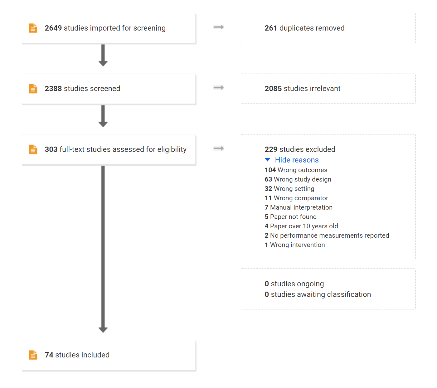
Figure 3 - Prisma results

Version	Author	Date
1473a05	Francisco Bischoff	2021-07-15

Meanwhile, the project pipeline has been set up on GitHub, Inc. ¹⁰ leveraging on Github Actions¹¹ for the Continuous Integration lifecycle. The repository is available at¹⁰, and the resulting report is available at⁸ for transparency while the roadmap and tasks are managed using the integrated Zenhub¹².

As it is known worldwide, since 2020, the measures taken to control the SARS-Cov2 pandemic have had a great impact on any development lifecycle.

At this moment, this project went through two timeline changes. In Fig. 4 it is shown the initial roadmap (as of May 2020), Fig. 5 the modified roadmap (as of July 2021), and Fig. 6 (as of Jan 2022). The literature survey is currently in the extraction phase, which includes about 74 articles from the full-text screening.

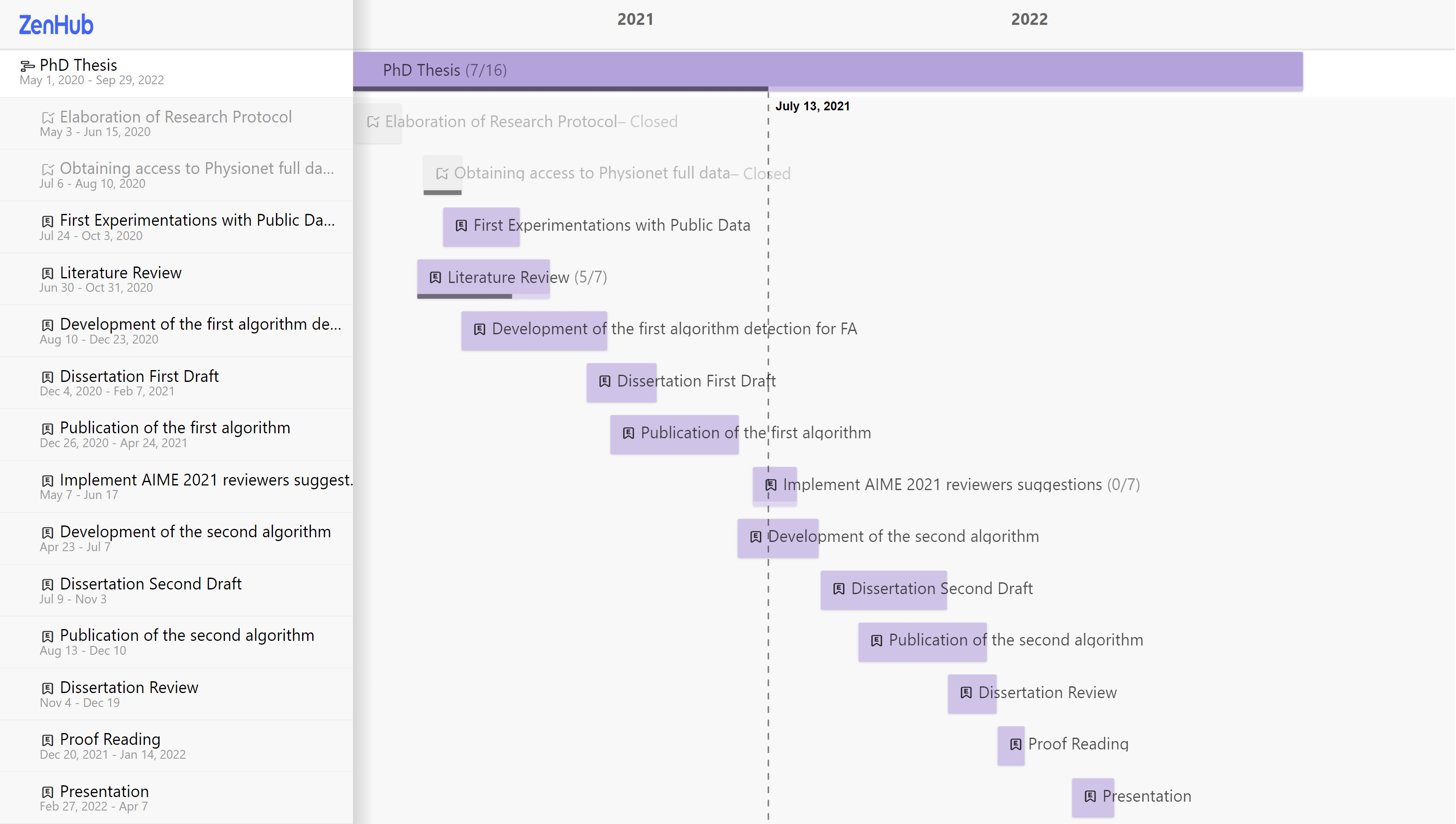
Figure 4 - Roadmap original

Version	Author	Date
1473a05	Francisco Bischoff	2021-07-15

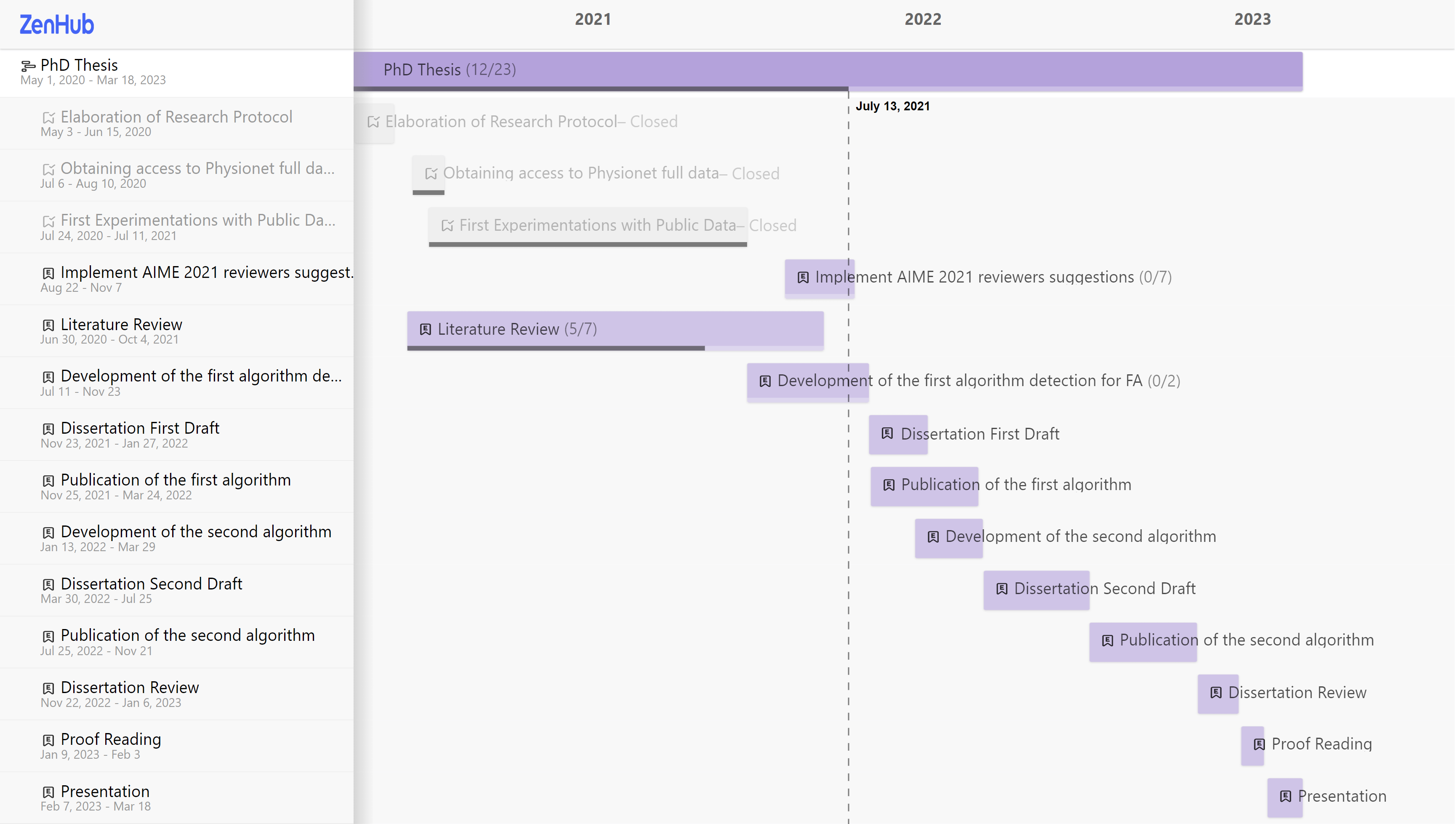
Figure 5 - Roadmap updated on August 2021

Version	Author	Date
1473a05	Francisco Bischoff	2021-07-15

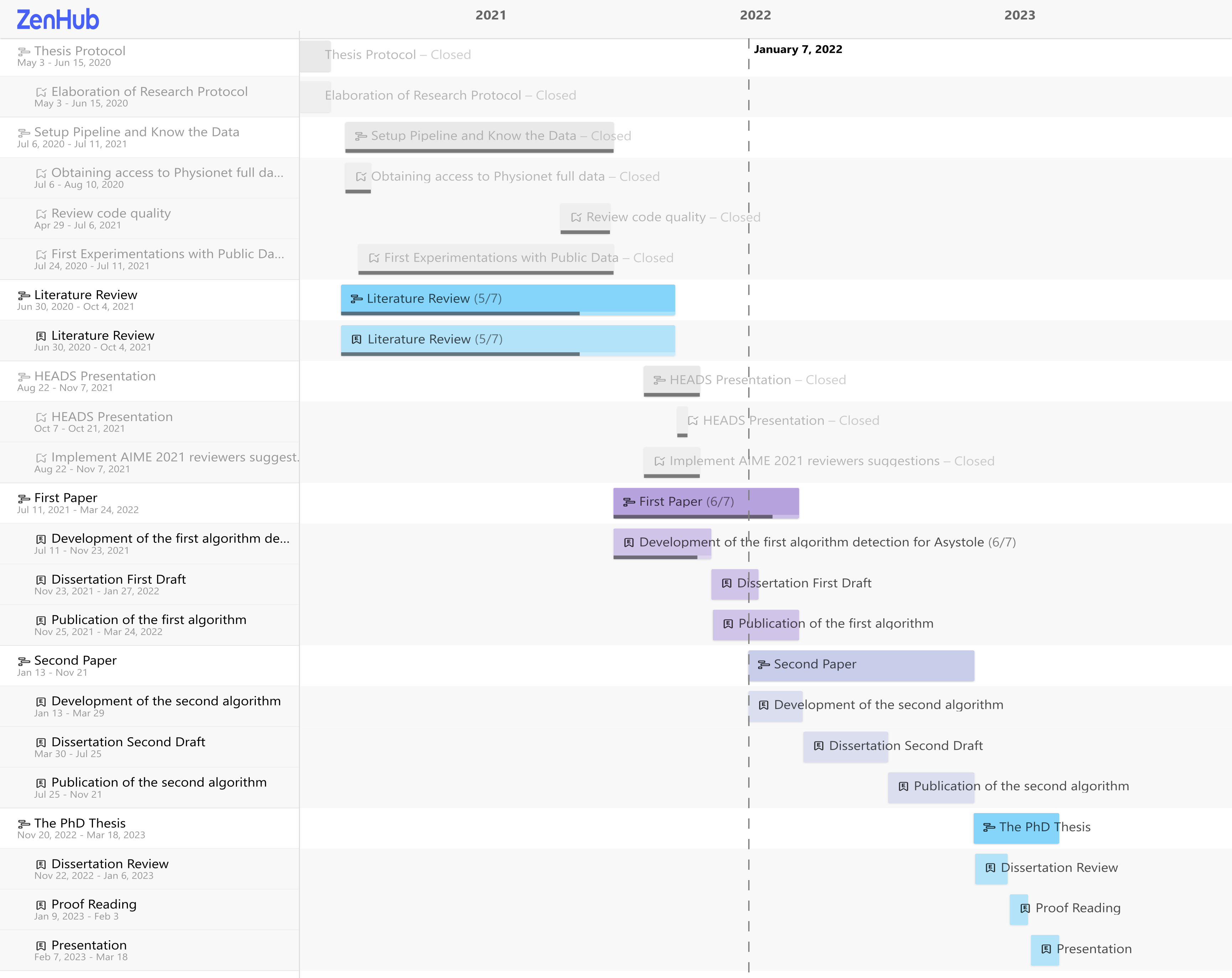
Figure 6 - Roadmap updated on January 2022

Version	Author	Date
571ac34	Francisco Bischoff	2022-01-15

1.4.2 Preliminary Experimentations

1.4.3 RAW Data

While programming the pipeline for the current dataset, it has been acquired a Single Lead Heart Rate Monitor breakout from Sparkfun^TM¹³ using the AD8232¹⁴ microchip from Analog Devices Inc., compatible with Arduino^(R)¹⁵, for an in-house experiment (Figs. 7 and 8).

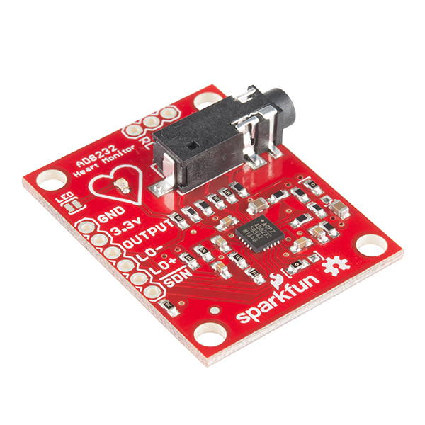
Figure 7 - Single Lead Heart Rate Monitor

Version	Author	Date
1473a05	Francisco Bischoff	2021-07-15

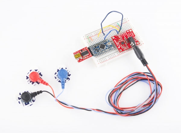
Figure 8 - Single Lead Heart Rate Monitor

Version	Author	Date
1473a05	Francisco Bischoff	2021-07-15

The output gives us a RAW signal as shown in Fig. 9.

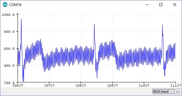
Figure 9 - RAW output from Arduino at ~300hz

Version	Author	Date
1473a05	Francisco Bischoff	2021-07-15

After applying the same settings as the Physionet database (collecting the data at 500hz, resample to 250hz, pass-filter, and notch filter), the signal is much better as shown in Fig. 10. Note: the leads were not placed on the correct location.

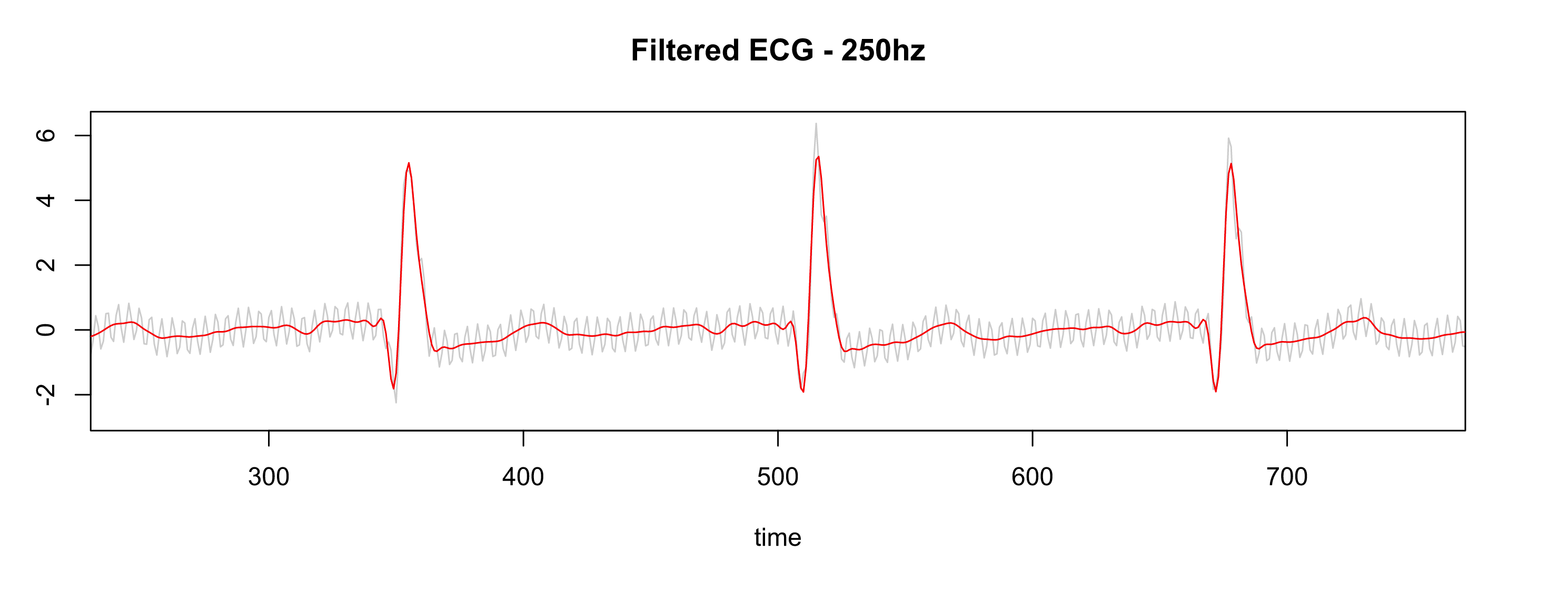
Figure 10 - Gray is RAW, Red is filtered

Version	Author	Date
1473a05	Francisco Bischoff	2021-07-15

So in this way, we allow us to import RAW data from other devices and build our own test dataset in the future.

1.4.3.1 Detecting Regime Changes

The regime change approach will be using the Arc Counts, as explained elsewhere¹⁶. The current implementation of the Matrix Profile in R, maintained by the first author of this thesis, is being used to accomplish the computations. This package was published in R Journal¹⁷.

A new concept was needed to be implemented on the algorithm in order to emulate (in this first iteration) the behavior of the real-time sensor: the search must only look for previous information within a time constraint. Thus, both the Matrix Profile computation and the Arc Counts needed to be adapted for this task.

At the same time, the ECG data needs to be “cleaned” for proper evaluation. That is different from the initial filtering process. Several SQIs (Signal Quality Indexes) are used on literature¹⁸, some trivial measures as kurtosis, skewness, median local noise level, other more complex as pcaSQI (the ratio of the sum of the five largest eigenvalues associated with the principal components over the sum of all eigenvalues obtained by principal component analysis applied to the time aligned ECG segments in the window). By experimentation (yet to be validated), a simple formula gives us the “complexity” of the signal and correlates well with the noisy data is shown in Equation \(\eqref{noise}\).

\[ \sqrt{\sum_{i=1}^w((x_{i+1}-x_i)^2)}, \quad \text{where}\; w \; \text{is the window size} \tag{1} \label{noise} \]

The Fig. 11 shows some SQIs.

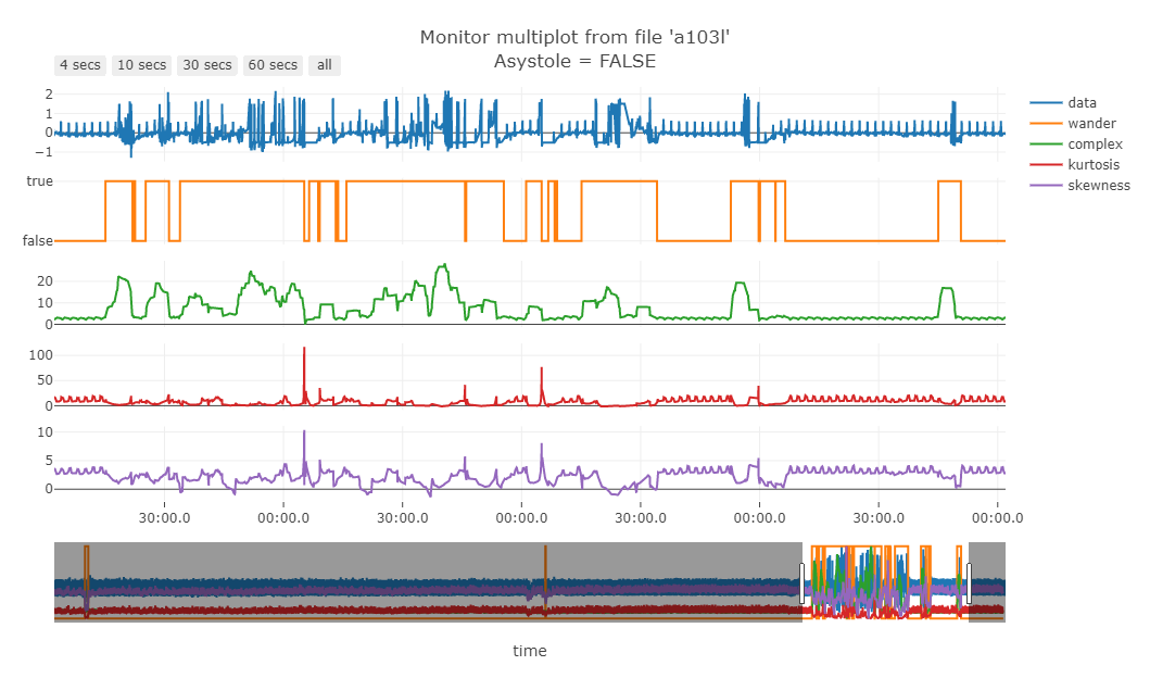
Figure 11 - Green line is the “complexity” of the signal

Version	Author	Date
1473a05	Francisco Bischoff	2021-07-15

Finally, a sample of the regime change detection is shown in Figs. 12 to 13.

Fig. 12 shows that noisy data (probably patient muscle movements) are marked with a blue point and thus are ignored by the algorithm. Also, valid for the following plots, the green and red lines on the data mark the 10 seconds window where the “event” that triggers the alarm is supposed to happen.

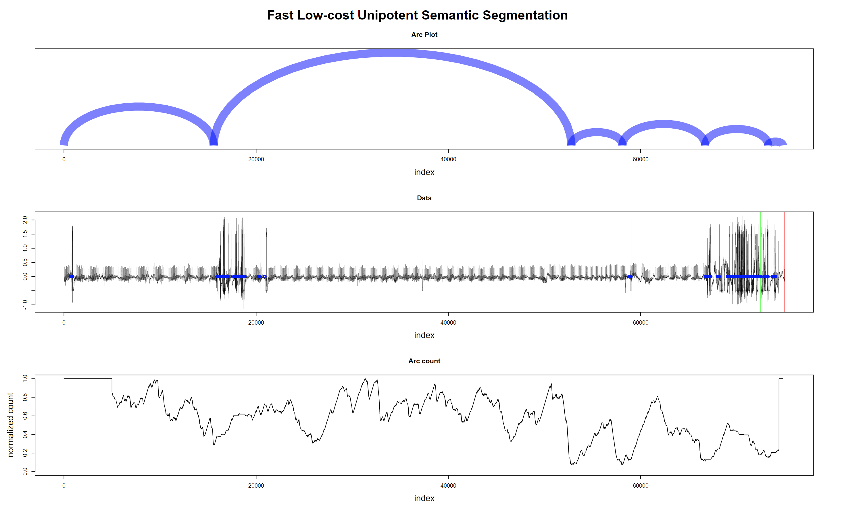
Figure 12 - Regime changes with noisy data - false alarm

Version	Author	Date
1473a05	Francisco Bischoff	2021-07-15

In Fig. 14, the data is clean; thus, nothing is excluded. Interestingly one of the detected regime changes is inside the “green-red” window. But it is a false alarm.

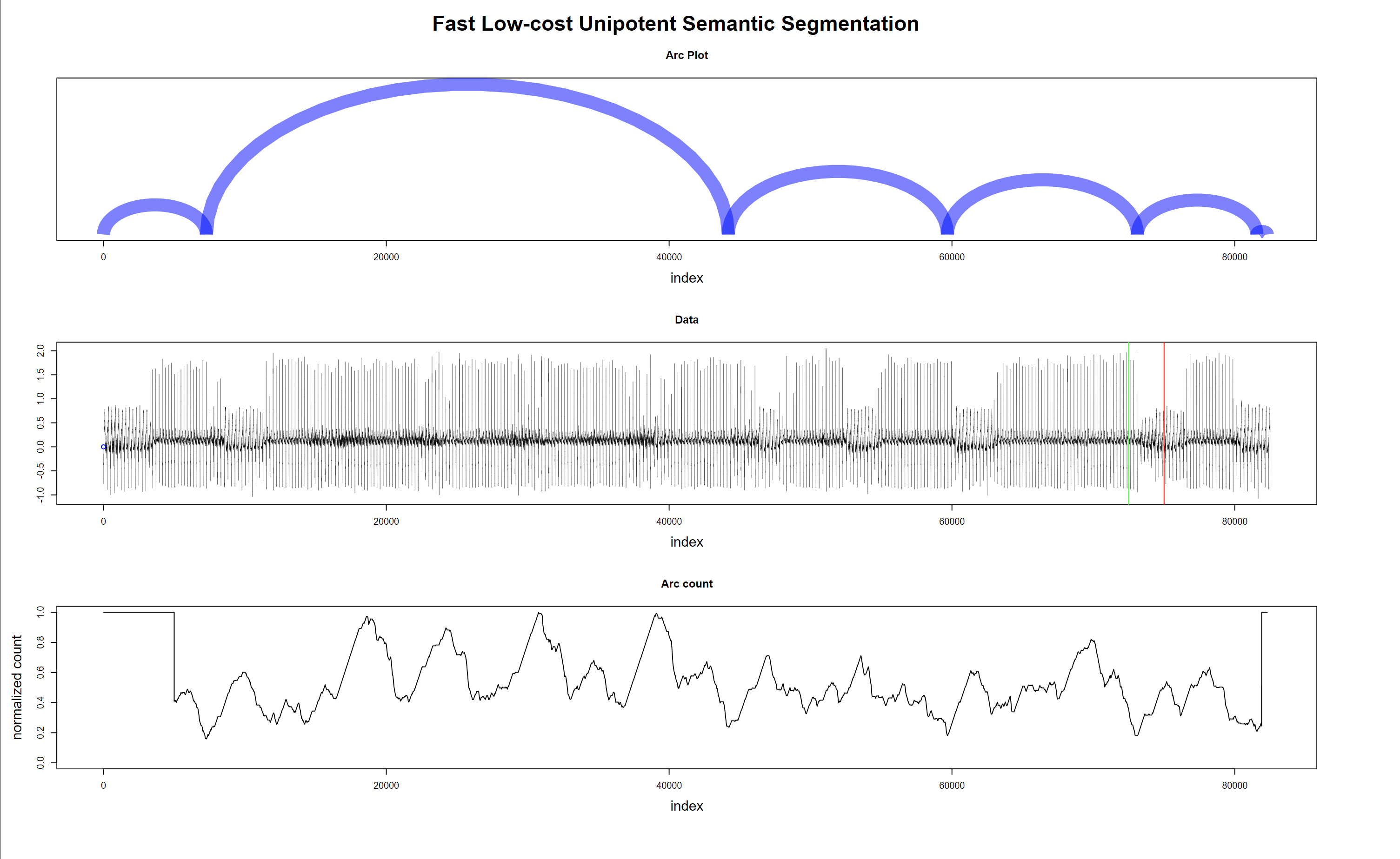
Figure 14 - Regime changes with good data - false alarm

Version	Author	Date
1473a05	Francisco Bischoff	2021-07-15

The last plot (Fig. 13) shows the algorithm’s robustness, not excluding good data with a wandering baseline, and the last regime change is correctly detected inside the “green-red” window.

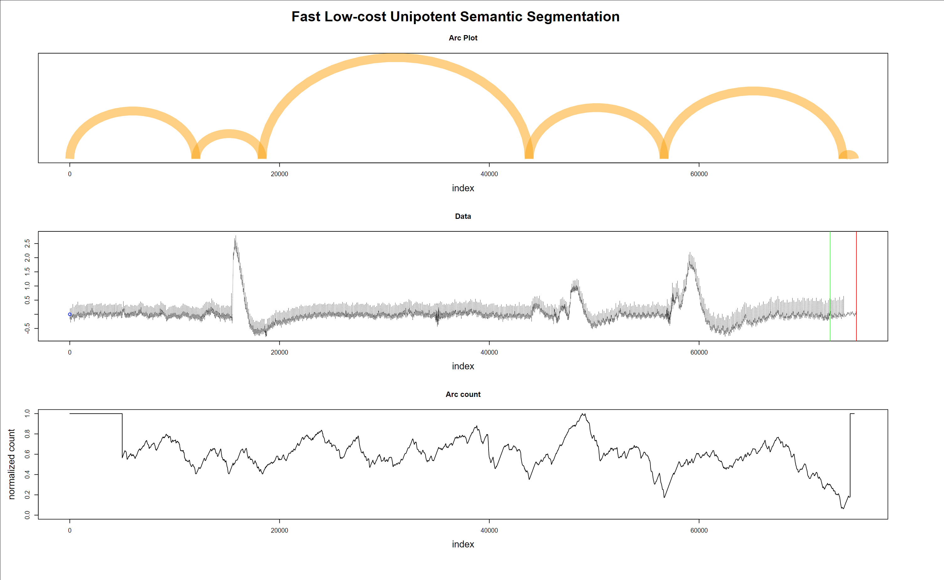
Figure 13 - Regime changes with good but wandering data - true alarm

Version	Author	Date
1473a05	Francisco Bischoff	2021-07-15

1.4.4 First General Assessment

By August 2021, it was clear that the chosen regime detection algorithm would be the (Fast Low-cost Online Semantic Segmentation) FLOSS¹⁹. Thus, the pipeline had to be adapted in order to allow the careful replication of the streaming process, even though several computations are made beforehand to keep the pipeline (i.e., the simulation) fast on exploring several parameters.

The choice of FLOSS is founded on the following arguments:

Domain Agnosticism: the algorithm makes no assumptions about the data as opposed to most available algorithms to date.
Streaming: the algorithm can provide real-time information.
Real-World Data Suitability: the objective is not to explain all the data. Therefore, areas marked as “don’t know” areas are acceptable.
FLOSS is not: a change point detection algorithm²⁰. The interest here is changes in the shapes of a sequence of measurements.

Other algorithms we can cite are based on Hidden Markov Models (HMM) that require at least two parameters set by domain experts: cardinality and dimensionality reduction. The most attractive alternative could be the Autoplait²¹, which is also domain agnostic and parameter-free. It segments the time series using Minimum Description Length (MDL) and recursively tests if the region is best modeled by one or two HMM. However, Autoplait is designed for batch operation, not streaming, and also requires discrete data. FLOSS was demonstrated to be superior in several datasets in its original paper. In addition, FLOSS is robust to several changes in data like downsampling, bit depth reduction, baseline wandering, noise, smoothing, and even deleting 3% of the data and filling with simple interpolation. Finally, the algorithm is light and suitable for low-power devices.

It is worth also mentioning the Time Series Snippets²², based on MPdist²³. The latter measures the distance between two sequences considering how many similar sub-sequences they share, no matter the order of matching. It proved to be a useful measure (not a metric) for meaningfully clustering similar sequences. Time Series Snippets exploits MPdist properties to summarize a dataset that contains representative sequences. This seems to be an alternative for detecting regime changes, but it is not. The purpose of this algorithm is to find which pattern(s) explains most of the dataset. Lastly, MPdist is quite expensive compared to the trivial Euclidean distance.

1.4.5 Second General Assessment

By January 2022, the following tasks were performed:

Restructuring the roadmap (again)
Refining the main pipeline (again)
Preparing for modeling and parameter tuning
Feasibility trial
And others

1.4.5.1 Refining the main pipeline

That can also be thought of as “rethinking” the pipeline. Which also leads to the roadmap restructuration. The new roadmap was already shown above in Fig. 6.

It is essential not only to write a pipeline that can “autoplot” itself for fine-grain inspection but also to design a high-level graph that can explain it “in a glance”. This exercise was helpful both ways: telling the story in a short version also reveals missing things and misleading paths that are not so obvious when thinking “low-level”.

Figs. 15, 16 and 17 show the overview of the processes involved.

Figure 15 - Pipeline for regime change detection

Version	Author	Date
571ac34	Francisco Bischoff	2022-01-15

Figure 16 - Pipeline for TRUE and FALSE alarm classification

Version	Author	Date
571ac34	Francisco Bischoff	2022-01-15

Figure 17 - Pipeline of the final process

Version	Author	Date
571ac34	Francisco Bischoff	2022-01-15

1.4.5.2 Preparing for modeling and parameter tuning

Here is one missing part that should have been addressed (formally) earlier. Although this work has its purpose of being finally deployed on small hardware, this prospective phase will need several hours of computing, tuning, evaluation, and validation of all findings.

Thus it was necessary to revisit the frameworks we are used to working on R: caret²⁴ and the newest tidymodels²⁵ collection. For sure, there are other frameworks and opinions²⁶. Notwithstanding, this project will follow the tidymodels road. Two significant arguments 1) constantly improving and constantly being re-checked for bugs; large community contribution; 2) allows to plug in a custom modeling algorithm that, in this case, will be the one needed for developing this work.

1.4.5.3 Feasibility trial

A side-project called “false.alarm.io” has been derived from this work (an unfortunate mix of “false.alarm” and “PlatformIO”²⁷, the IDE chosen to interface the panoply of embedded systems we can experiment with). The current results of this side-project are very enlightening and show that the final algorithm can indeed be used in small hardware. Further data will be available in the future.

1.4.5.4 And others

After this “step back” to look forward, it was time to define how the regime change algorithm would integrate with the actual decision of triggering or not the alarm. Some hypotheses were thought out: (1) clustering similar patterns, (2) anomaly detection, (3) classification, and (4) forecasting. Among these methods, it was thought, in order to avoid exceeding processor capacity, an initial set of shapelets²⁸ can be sufficient to rule in or out the TRUE/FALSE challenge. Depending on the accuracy of this approach and the resources available, another method can be introduced for both (1) improving the “negative”¹ samples and (2) learning more shapelets to improve the TRUE/FALSE alarm discrimination.

1.4.6 Scientific Contributions

On regime change detection: in the original paper, the FLOSS algorithm assumes the Arc Counts follow a “uniform distribution” when we add a temporal constraint (not considering arcs coming from older data), and the Arc Counts of newly incoming data are truncated by the same amount of temporal constraint. This prevents completely the detection of a regime change in the last 10 seconds as required. This issue is overcome using the theoretical distributions as shown in Fig. 18.
On the Matrix Profile: since the first paper presenting this new concept²⁹, lots of investigations were made to speed up its computation. It is notable how all computations are not dependent on the rolling window size as previous works not using Matrix Profile. Aside from this, we can see that the first STAMP²⁹ algorithm has the time complexity of \(O(n^2log{n})\) while STOMP³⁰ \(O(n^2)\) (a significant improvement), but STOMP lacks the “any-time” property. Later SCRIMP³¹ solves this problem keeping the same time complexity of \(O(n^2)\). Here we are in the “exact” algorithms domain and will not extend the scope for conciseness.
1. The main issue with the algorithms above is the dependency on a fast Fourier transform (FFT) library. FFT has been extensively optimized and architecture/CPU bounded to exploit the most of speed. Also, padding data to some power of 2 happens to increase the efficiency of the algorithm. We can argue that time complexity doesn’t mean “faster” when we can exploit low-level instructions. In our case, using FFT in a low-power device is overkilling. For example, a quick search over the internet gives us a hint that computing FFT on a 4096 data in an ESP32 takes about 21ms (~47 computations in 1 second). This means ~79 seconds for computing all FFT’s (~3797) required for STAMP using a window of 300. Currently, we can compute 50k full matrices in less time using no FFT in an ESP32 MCU (Fig. 19).
2. Recent works using exact algorithms are using an unpublished algorithm called MPX, which computes the Matrix Profile using cross-correlation methods ending up faster and is easily portable.
3. The main contribution of this work on this area is adding the online capability to MPX, which means we can update the Matrix Profile as new data comes in.
On extending the Matrix Profile: an unexplored constraint that we could apply on building the Matrix Profile we are calling Similarity Threshold (ST). The original work outputs the similarity values in Euclidean Distance (ED) values, while MPX naturally outputs the values in Pearson’s correlation coefficients (CC). Both ED and CC are interchangeable using the equation \(\eqref{edcc}\). However, we may argue that it is easier to compare values that do not depend on the window size during an exploratory phase. MPX happens to naturally return values in CC, saving a few more computation time. The ST is an interesting factor that we can use, especially when detecting pattern changes during time. The FLOSS algorithm relies on counting references between indexes in the time series. ST can help remove “noise” from these references since only similar patterns above a certain threshold are referenced, and changes have more impact on these counts. The best ST threshold is still to be determined.

\[ CC = 1 - \frac{ED}{(2 \times WindowSize)} \tag{2} \label{edcc} \]

Figure 18 - 1D-IAC distributions for earlier temporal constraint (on Matrix Profile)

Version	Author	Date
571ac34	Francisco Bischoff	2022-01-15

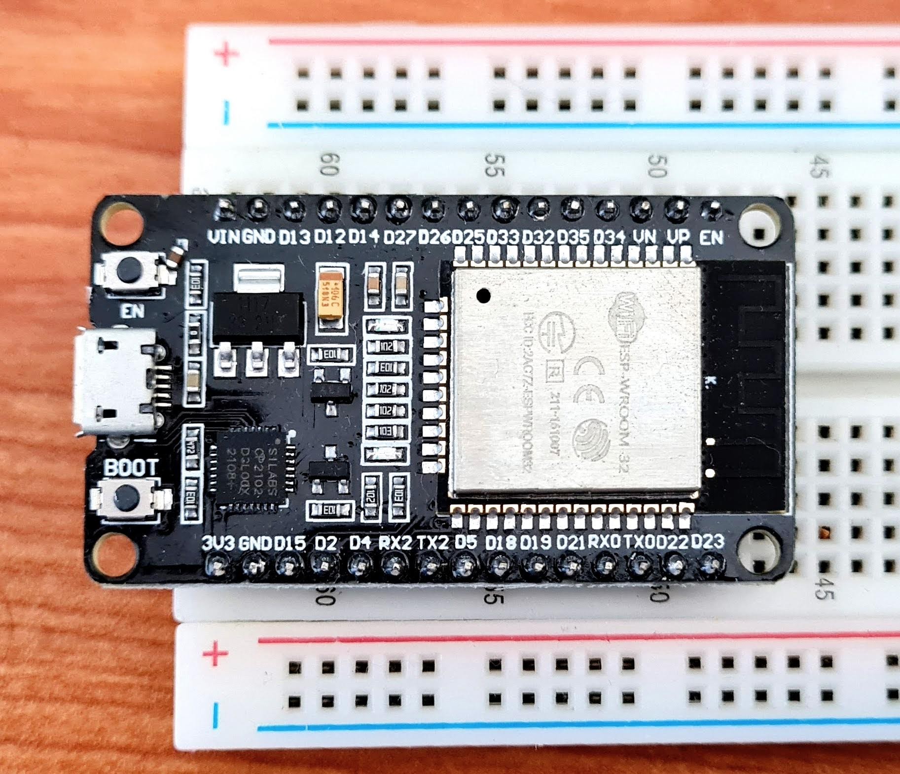
Figure 19 - ESP32 MCU

Version	Author	Date
571ac34	Francisco Bischoff	2022-01-15

1. Research compendium. Published 2019. Accessed April 8, 2021. https://research-compendium.science

2. Wilkinson M, Dumontier M, Aalbersberg I, et al. The fair guiding principles for scientific data management and stewardship. Scientific Data. 2016;3(1). doi:10.1038/sdata.2016.18

3. The codemeta project. Published 2017. Accessed January 10, 2022. https://codemeta.github.io/

4. Reducing false arrhythmia alarms in the icu - the physionet computing in cardiology challenge 2015. Published online March 24, 2021. doi:10.5281/zenodo.4634013

5. Clifford GD, Silva I, Moody B, et al. The physionet/computing in cardiology challenge 2015: Reducing false arrhythmia alarms in the icu. In: Computing in Cardiology.; 2015. doi:10.1109/cic.2015.7408639

6. Association for the Advancement of Medical Instrumentation. Cardiac monitors, heart rate meters, and alarms. Association for the Advancement of Medical Instrumentation; 2002.

7. Landau W, Landau W, Warkentin M, et al. Ropensci/Targets, Dynamic Function-Oriented ’Make’-Like Declarative Workflows. Zenodo; 2021. doi:10.5281/ZENODO.4062936

8. Franzbischoff/false.alarm: Reproducible reports. Published 2021. Accessed April 8, 2021. https://franzbischoff.github.io/false.alarm

9. Blischak JD, Carbonetto P, Stephens M. Creating and sharing reproducible research code the workflowr way [version 1; peer review: 3 approved]. F1000Research. 2019;8(1749). doi:10.12688/f1000research.20843.1

10. Bischoff F. GitHub false.alarm repository. Accessed July 14, 2021. https://github.com/franzbischoff/false.alarm

11. GitHub Actions. Accessed July 14, 2021. https://github.com/features/actions

12. Zenhub workspace. Accessed July 14, 2021. https://app.zenhub.com/workspaces/phd-thesis-5eb2ce34f5f30b3aed0a35af/board

13. SparkFun Single Lead Heart Rate Monitor - AD8232 - SEN-12650 - SparkFun Electronics. Accessed July 14, 2021. https://www.sparkfun.com/products/12650

14. Analog Devices. AD8232 Single-Lead, Heart Rate Monitor Front End. Published online 2020. Accessed July 14, 2021. https://www.analog.com/media/en/technical-documentation/data-sheets/ad8232.pdf

15. Arduino. Accessed July 14, 2021. https://www.arduino.cc/

16. Gharghabi S, Yeh C, Ding Y, et al. Domain agnostic online semantic segmentation for multi-dimensional time series. Data Mining and Knowledge Discovery. 2018;33(1):96-130. doi:10.1007/s10618-018-0589-3

17. Bischoff F, Rodrigues PP. tsmp: An R Package for Time Series with Matrix Profile. The R Journal. 2020;12(1):76-86. doi:10.32614/RJ-2020-021

18. Eerikainen L, Vanschoren J, Rooijakkers M, Vullings R, Aarts R. 2015 computing in cardiology conference (cinc). In: IEEE; 2015. doi:10.1109/cic.2015.7408644

19. Gharghabi S, Ding Y, Yeh C-CM, Kamgar K, Ulanova L, Keogh E. 2017 ieee international conference on data mining (icdm). In: IEEE; 2017. doi:10.1109/icdm.2017.21

20. Aminikhanghahi S, Cook DJ. A survey of methods for time series change point detection. Knowledge and Information Systems. 2016;51(2):339-367. doi:10.1007/s10115-016-0987-z

21. Matsubara Y, Sakurai Y, Faloutsos C. AutoPlait: Automatic mining of co-evolving time sequences. Proceedings of the ACM SIGMOD International Conference on Management of Data. Published online 2014:193-204. doi:10.1145/2588555.2588556

22. Imani S, Madrid F, Ding W, Crouter S, Keogh E. Matrix profile xiii : Time series snippets : A new primitive for time series data mining. In: 2018 Ieee International Conference on Data Mining (Icdm).; 2018.

23. Gharghabi S, Imani S, Bagnall A, Darvishzadeh A, Keogh E. Matrix profile xii: MPdist: A novel time series distance measure to allow data mining in more challenging scenarios. In: IEEE; 2018:965-970. doi:10.1109/ICDM.2018.00119

24. Kuhn M. Building predictive models in r using the caret package. Journal of Statistical Software, Articles. 2008;28(5):1-26. doi:10.18637/jss.v028.i05

25. Kuhn M, Wickham H. Tidymodels: A Collection of Packages for Modeling and Machine Learning Using Tidyverse Principles.; 2020. https://www.tidymodels.org

26. Thompson J. On not using tidymodels. Published October 2020. Accessed January 5, 2022. https://staffblogs.le.ac.uk/teachingr/2020/10/05/on-not-using-tidymodels/

27. PlatformIO, a professional collaborative platform for embedded development. Accessed January 5, 2022. https://platformio.org/

28. Rakthanmanon T, Keogh E. Fast shapelets: A scalable algorithm for discovering time series shapelets. In: Proceedings of the 2013 Siam International Conference on Data Mining. Society for Industrial; Applied Mathematics; 2013:668-676. doi:10.1137/1.9781611972832.74

29. Yeh C-CM, Zhu Y, Ulanova L, et al. Matrix profile i: All pairs similarity joins for time series: A unifying view that includes motifs, discords and shapelets. In: 2016 Ieee 16th International Conference on Data Mining (Icdm). IEEE; 2016:1317-1322. doi:10.1109/ICDM.2016.0179

30. Zhu Y, Zimmerman Z, Senobari NS, et al. 2016 ieee 16th international conference on data mining (icdm). In: IEEE; 2016. doi:10.1109/icdm.2016.0085

31. Zhu Y, Yeh C-CM, Zimmerman Z, Kamgar K, Keogh E. 2018 ieee international conference on data mining (icdm). In: IEEE; 2018. doi:10.1109/icdm.2018.00099

R version 4.1.2 (2021-11-01)
Platform: x86_64-pc-linux-gnu (64-bit)
Running under: Ubuntu 20.04.3 LTS

Matrix products: default
BLAS:   /usr/lib/x86_64-linux-gnu/blas/libblas.so.3.9.0
LAPACK: /usr/lib/x86_64-linux-gnu/lapack/liblapack.so.3.9.0

locale:
 [1] LC_CTYPE=C.UTF-8       LC_NUMERIC=C           LC_TIME=C.UTF-8       
 [4] LC_COLLATE=C.UTF-8     LC_MONETARY=C.UTF-8    LC_MESSAGES=C.UTF-8   
 [7] LC_PAPER=C.UTF-8       LC_NAME=C              LC_ADDRESS=C          
[10] LC_TELEPHONE=C         LC_MEASUREMENT=C.UTF-8 LC_IDENTIFICATION=C   

attached base packages:
[1] stats     graphics  grDevices datasets  utils     methods   base     

other attached packages:
 [1] stringr_1.4.0     ggplot2_3.3.5     gridExtra_2.3     kableExtra_1.3.4 
 [5] tibble_3.1.6      visNetwork_2.1.0  gittargets_0.0.1  tarchetypes_0.4.1
 [9] targets_0.10.0    workflowr_1.7.0   here_1.0.1       

loaded via a namespace (and not attached):
 [1] Rcpp_1.0.8            gert_1.5.0            svglite_2.0.0.9000   
 [4] languageserver_0.3.12 getPass_0.2-2         ps_1.6.0             
 [7] rprojroot_2.0.2       digest_0.6.29         utf8_1.2.2           
[10] R6_2.5.1              backports_1.4.1       sys_3.4              
[13] evaluate_0.14         highr_0.9             httr_1.4.2           
[16] pillar_1.6.4          rlang_0.99.0.9003     uuid_1.0-3           
[19] rstudioapi_0.13       data.table_1.14.2     whisker_0.4          
[22] callr_3.7.0           jquerylib_0.1.4       rmarkdown_2.11       
[25] labeling_0.4.2        webshot_0.5.2         htmlwidgets_1.5.4    
[28] igraph_1.2.11         munsell_0.5.0         compiler_4.1.2       
[31] httpuv_1.6.5          xfun_0.29             systemfonts_1.0.3    
[34] pkgconfig_2.0.3       askpass_1.1           htmltools_0.5.2      
[37] openssl_1.4.6         tidyselect_1.1.1      codetools_0.2-18     
[40] viridisLite_0.4.0     fansi_1.0.2           crayon_1.4.2         
[43] dplyr_1.0.7           withr_2.4.3           later_1.3.0          
[46] grid_4.1.2            gtable_0.3.0          jsonlite_1.7.2       
[49] lifecycle_1.0.1       git2r_0.29.0          magrittr_2.0.1       
[52] credentials_1.3.2     scales_1.1.1          cli_3.1.0            
[55] stringi_1.7.6         debugme_1.1.0         farver_2.1.0         
[58] renv_0.15.1           fs_1.5.2              promises_1.2.0.1     
[61] xml2_1.3.3            bslib_0.3.1           ellipsis_0.3.2       
[64] generics_0.1.1        vctrs_0.3.8           tools_4.1.2          
[67] glue_1.6.0            purrr_0.3.4           processx_3.5.2       
[70] fastmap_1.1.0         yaml_2.2.1            colorspace_2.0-2     
[73] base64url_1.4         rvest_1.0.2           knitr_1.37           
[76] sass_0.4.0

The term “negative” does not imply that the patient has a “normal” ECG. It means that the “negative” section is not a life-threatening condition that needs to trigger an alarm.↩

Report

Francisco Bischoff

on Jan 15, 2022