Last updated: 2021-05-12
Checks: 7 0
Knit directory:
thesis/analysis/
This reproducible R Markdown analysis was created with workflowr (version 1.6.2). The Checks tab describes the reproducibility checks that were applied when the results were created. The Past versions tab lists the development history.
Great! Since the R Markdown file has been committed to the Git repository, you know the exact version of the code that produced these results.
Great job! The global environment was empty. Objects defined in the global environment can affect the analysis in your R Markdown file in unknown ways. For reproduciblity it’s best to always run the code in an empty environment.
The command set.seed(20210321) was run prior to running the code in the R Markdown file.
Setting a seed ensures that any results that rely on randomness,
e.g. subsampling or permutations, are reproducible.
Great job! Recording the operating system, R version, and package versions is critical for reproducibility.
Nice! There were no cached chunks for this analysis, so you can be confident that you successfully produced the results during this run.
Great job! Using relative paths to the files within your workflowr project makes it easier to run your code on other machines.
Great! You are using Git for version control. Tracking code development and connecting the code version to the results is critical for reproducibility.
The results in this page were generated with repository version 7fd4ff2. See the Past versions tab to see a history of the changes made to the R Markdown and HTML files.
Note that you need to be careful to ensure that all relevant files for the
analysis have been committed to Git prior to generating the results (you can
use wflow_publish or wflow_git_commit). workflowr only
checks the R Markdown file, but you know if there are other scripts or data
files that it depends on. Below is the status of the Git repository when the
results were generated:
Ignored files:
    Ignored:    .Rproj.user/
    Ignored:    data/DB/
    Ignored:    data/raster/
    Ignored:    data/raw/
    Ignored:    data/vector/
    Ignored:    docker_command.txt
    Ignored:    output/acc/
    Ignored:    output/bayes/
    Ignored:    output/ffs/
    Ignored:    output/models/
    Ignored:    output/plots/
    Ignored:    output/test-results/
    Ignored:    renv/library/
    Ignored:    renv/staging/
    Ignored:    report/presentation/

Untracked files:
    Untracked:  analysis/assets/
Note that any generated files, e.g. HTML, png, CSS, etc., are not included in this status report because it is ok for generated content to have uncommitted changes.
These are the previous versions of the repository in which changes were made
to the R Markdown (analysis/thesis-methods.Rmd) and HTML (docs/thesis-methods.html)
files. If you’ve configured a remote Git repository (see
?wflow_git_remote), click on the hyperlinks in the table below to
view the files as they were in that past version.
| File | Version | Author | Date | Message |
|---|---|---|---|---|
| Rmd | 7fd4ff2 | Darius Görgen | 2021-05-12 | workflowr::wflow_publish(files = list.files(“.”, “Rmd$”)) |
| Rmd | de8ce5a | Darius Görgen | 2021-04-05 | add content |
| html | de8ce5a | Darius Görgen | 2021-04-05 | add content |
1 Methods
1.1 Model Specifications
In the following section, the model specifications and the training and validation procedures are outlined. The core model of this thesis consists of a Convolutional-Long-Short-Term-Memory Neural Network (CNN-LSTM). However, as a baseline reference to asses the CNN-LSTM performance, a standard logistic regression model (LR) is also constructed. Starting from the LR model, relevant concepts for the establishment of the training architecture are introduced.
1.1.1 Logistic Regression
LR models have been the standard in conflict research for some time. One advantage of regression models is that the model outcome is easy to interpret by humans, which is of primary importance when research results are used to inform policy decisions. Recently, Halkia et al. (2020) published the methodology for the GCRI developed for the European Union Conflict Early Warning System which is based on LR. Their model outperforms or achieves comparable accuracy metrics compared to several conflict prediction tools based on more complex modeling procedures. This indicates that a LR model constitutes a viable choice to compare it with the results of more advanced modeling techniques such as neural networks. A binomial LR predicts the probability of an observation belonging to either one of two categories of a dichotomous dependent variable based on a number of independent variables following Equation (1.1).
\[\begin{equation} P(Y) = \frac{e^\gamma}{1+e^\gamma}; \gamma = \beta_0 + \beta_1x_1 + \beta_2x_2 + ... +\beta_nx_n \tag{1.1} \end{equation}\]
In this form, \(P(Y)\) will take a value between 0 and 1 and represents the probability of a conflict occurrence. \(x_1 ... x_n\) represent the predictor variables while \(\beta_0 ... \beta_n\) represent the model coefficients to be fitted. From the equation, it becomes evident that logistic regressions assume a linear relationship between the predictors and the response variable. Secondly, LR is not intrinsically designed to handle a time axis, even though one could include time as an additional independent variable. It also means that LR can only produce one output at a time for each observation. If one wants to predict conflict for several months into the future, a specific model must be trained for each month in the prediction horizon.
Additionally, LR models are highly sensitive to class imbalances in the training data set. Conflict prediction is a classification task with a very high class imbalance (Table ??). Various techniques exist to cope with class imbalance (Ali et al., 2015). One among them which has been previously used in conflict research is downsampling (Hegre et al., 2019). Here, before fitting the model, the majority class, which is represented by non-conflict district-months, is randomly downsampled to match the size of the minority class. This balanced subset is then used to fit the model parameters. Metric evaluations can be applied on a hold-out test data set, characterized by the original imbalanced distribution between conflict and non-conflict district months. The procedure to map the probabilistic model output to a binary classification follows Equation (1.2):
\[\begin{equation} \hat{Y} = \begin{cases} 1 & \text{if } P(Y) \geq \lambda \\ 0 & \text{otherwise} \end{cases} \tag{1.2} \end{equation}\]
Here, \(\lambda\) is a threshold value usually selected to be \(0.5\). However, specifically in modeling tasks with a high class imbalance such as conflict prediction, an optimal threshold might be searched for a given accuracy metric - a process referred to as threshold tuning (Zou et al., 2016).
1.1.2 CNN-LSTM
1.2 Basic Concepts of Neural Networks.
Before explaining the fundamentals of CNN-LSTMs, a first step is to define the modeling task which might guide the reader through the descriptions to follow. In the present case, the modeling task is one of a multivariate time series prediction with a multi-step prediction horizon. The available training data set can be formally described as in Equation (1.3),
\[\begin{equation} X_t^L= x_t^1,x_{t+1}^1...,x_{t-N+1}^1,...\ ..., x_t^L,...,x_{t-N+1}^L \tag{1.3} \end{equation}\]
where \(X_t^L\) is the predictor matrix with \(L\) predictors and \(t\) available timesteps. The training process then comprises the search for a function \(f(X_t^L)\) which maps the input features to a multi-step prediction vector following Equation (1.4),
\[\begin{equation} \hat{Y} = f(X_t^L) = {\hat{y}_{t+1},\hat{y}_{t+2},...,\hat{y}_{t+h}} \tag{1.4} \end{equation}\]
where \(\hat{Y}\) is the predicted outcome vector of \(h\) time steps into the future. Commonly, the modeling function is trained on equal length inputs, such as the last 24 hours for energy price forecasting (Cordoni, 2020), the last week in the case of particle matter concentration forecasting (Li et al., 2020), or even several years worth of data in the case of solar irradiance and photovoltaic power prediction (Rajagukguk et al., 2020). However, sophisticated deep learning models are also able to model variable-length inputs to variable-length outputs, i.e., in the case of language translation models (Yang et al., 2020).
The most fundamental concept in neural networks is that of a single neuron. This neuron receives some inputs \(X\), learns a weight matrix \(W\) which then is used for a multiplicative interaction with the inputs, and an additional bias term \(b\) is added. The final output \(\hat{Y}\) is obtained by passing the results of this interaction through a possibly non-linear activation function, also called activation function, here represented by a \(\sigma\)-function (1.5):
\[\begin{equation} \hat{Y} = \sigma \Big(WX+b \Big). \tag{1.5} \end{equation}\]
These predicted outcomes can be used to calculate the error in comparison to the observed outcomes based on a specific loss function also referred to as cost function \(C\). In a general notation, a given loss function calculates the loss between predicted and observed values which in itself is a function of the weights, the bias, the activation function and the inputs and observed values based on Equation (1.6):
\[\begin{equation} Loss = C(Y-\hat{Y}) = C(W b \sigma X Y). \tag{1.6} \end{equation}\]
The loss is used to adjust the weight matrix \(W\) and the bias term \(b\) to more precisely match the expected outputs. This is achieved through a process called backpropagation. It is the process governing how a network learns to optimize the model function from Equation (1.4). To apply backpropagation, partial derivatives of the loss function in relation to its components are calculated from the output towards the inputs. This way, the gradient of change in the loss conditioned by the single components can be estimated. The gradients’ calculation is not included in detail for brevity. However, a comprehensive explanation of the process can be found in Parr and Howard (2018).
In relation to the weight matrix \(W\), the gradients are defined by the partial derivatives of the loss in relation to the single weights according to Equation (1.7):
\[\begin{equation} \nabla{C_{W}} = \begin{bmatrix} \frac{\partial{C}}{\partial{w_1}} \\ \frac{\partial{C}}{\partial{w_2}} \\ \vdots \\ \frac{\partial{C}}{\partial{w_n}} \end{bmatrix} \tag{1.7} \end{equation}\]
The gradients are used to update the weight matrix in the direction the loss function is suspected to decrease most rapidly following Equation (1.8)
\[\begin{equation} W^* = W - \eta \nabla{C_{W}}, \tag{1.8} \end{equation}\]
where \(\eta\) is a constant steering how much the weight matrix is adjusted in the gradients’ direction referred to as learning rate, and \(W^*\) is the adjusted weight matrix. The same principle applies to the bias term. It should be noted that the process of backpropagation described here is simplified to a single-layer network. For multi-layer networks, the error terms have to be backpropagated from one layer to the next, in the direction from the output layer towards the input layer. However, the general concept remains the same. In this context, it is essential to differentiate between different training strategies which differ from each other mainly by the fact when gradients are calculated, and weights are adjusted during training. The first is called batch gradient descent. Here the gradients are calculated on based on all available observations. Once all training samples have been passed through the network, the cost function evaluates the loss and the errors are then backpropagated to adjust the weight matrix and bias terms. The second strategy is referred to as stochastic gradient descent or online learning, where a backpropagation takes place for every single sample. The last one is called mini-batch gradient descent and is the most widely used strategy. Based on a pre-defined batch size, the training data set is separated into equally sized batches. Backpropagation is then applied once a batch has been passed through the network. Additionally, several functions governing the adaptation process exist. They are referred to as optimizers and they mainly differ in the way the learning rate is adapted during the training process. An analysis of these differences is out of this thesis’ scope, and the reader is referred to Sun et al. (2019) for a comprehensive overview.
1.3 Convolutional Neural Networks.
In contrast to the simple neural network structure explained in the section above, CNNs work by applying a convolution kernel to the inputs. This operation effectively summarizes the input values based on a specific number of different kernels with a shared kernel width (Figure 1.1). This behavior of CNNs made them most attractive to tasks involving 2D-data such as image classification (Krizhevsky et al., 2017) or the analysis of remote sensing imagery (Song et al., 2019). Despite this traditional usage, CNNs successfully have been employed with 1D data structures with a time-component such as audio signals (Lee et al., 2009), activity detection and heart failure (Zheng et al., 2014) or stock price forecasting (Mehtab et al., 2020).
bracket_text = tibble(x=4, y=5.8 , text=TeX("$\\beta = 3$"))
kernel = tibble(x = c(3:5), y = rep(5.5,3), text = TeX(paste("$w_{k,", 1:3, "}$", sep="")))
arrow = tibble(x=5.6, y=5.5, xend=6.5, yend=5.5)
points = tibble(x = 4.5, y = c(2.7,2.5,2.3))
anno_left = tibble(x=rep(-1,5), y = c(5.5,4.5, 3.5, 1.5, 0), text = TeX(c("$W_k$", "$L_1$", "$L_2$", "$L_i$", "$X^*_k$")))
input_1 = tibble(x = c(0:9), y = rep(4.5, 10), group = factor(c(0,1,1,2,2,2,rep(1,4)),
                                                              label = c("0","1","2","3","4"),
                                                              levels = 0:4),
                 text = c("0", TeX(paste("$x_", 1:7, "$", sep="")),"...", TeX("$x_t$")))

input_2 = tibble(x = c(0:9), y = rep(3.5, 10),  group = factor(c(0,1,1,2,2,2,rep(1,4)),
                                                               label = c("0","1","2","3","4"),
                                                               levels = 0:4),
                 text = c("0", TeX(paste("$x_", 1:7, "$", sep="")),"...", TeX("$x_t$")))

input_3 = tibble(x = c(0:9), y = rep(1.5, 10),  group = factor(c(0,1,1,2,2,2,rep(1,4)),
                                                               label = c("0","1","2","3","4"),
                                                               levels = 0:4),
                 text = c("0", TeX(paste("$x_", 1:7, "$", sep="")),"...", TeX("$x_t$")))

output = tibble(x = c(1:9), y = rep(0, 9), group = factor(c(3,3,3,2,rep(4,5)),
                                                          label = c("0","1","2","3","4"),
                                                          levels = 0:4),
                text = c(TeX(paste("$y_{k,", 1:4, "}$", sep="")), rep("",5)))

ggplot() +
  annotate(geom="text", x=4, y=6.5, label=TeX("$\\beta = 3$"), size=5, parse=TRUE)+
  # annotate(geom="text", x=4, y=6, label=TeX("$\\{$"), parse=TRUE, angle=-90, size=50)+
  geom_rect(data=kernel, aes(xmin=x-.5, xmax=x+.5, ymin=y-.4, ymax=y+.4),
            fill = "#E6AB02",color = "black") +
  geom_text(data=kernel, aes(x=x, y=y, label=text),
            parse=T, size=4.5) +
  geom_segment(data=arrow, aes(x=x,y=y,xend=xend,yend=yend),
               arrow = arrow(length=unit(0.5,"cm")), size = 1) +
  geom_rect(data=input_1, aes(xmin=x-.5, xmax=x+.5, ymin=y-.4, ymax=y+.4, fill=group),
            color = "black", show.legend = F) +
  geom_text(data=input_1, aes(x=x,y=y,label=text), parse=T, size=4.5) +
  geom_point(data=points, aes(x=x,y=y)) +
  geom_rect(data=input_2, aes(xmin=x-.5, xmax=x+.5, ymin=y-.4, ymax=y+.4, fill=group),
            color = "black", show.legend = F) +
  geom_text(data=input_2, aes(x=x,y=y,label=text), parse=T, size=4.5) +
  geom_rect(data=input_3, aes(xmin=x-.5, xmax=x+.5, ymin=y-.4, ymax=y+.4, fill=group),
            color = "black", show.legend = F) +
  geom_text(data=input_3, aes(x=x,y=y,label=text), parse=T, size=4.5) +
  geom_rect(data=output, aes(xmin=x-.5, xmax=x+.5, ymin=y-.4, ymax=y+.4, fill=group),
            color = "black", show.legend = F) +
  geom_text(data=output, aes(x=x,y=y,label=text), parse=T, size=4.5) +
  geom_text(data=anno_left, aes(x=x,y=y,label=text), parse=T, size=6) +
  scale_fill_manual(values=c("#999999","#7570B3","#E6AB02","#1B9E77","transparent")) +
  theme_classic() +
  ylim(-1,7) +
  labs(x=NULL, y=NULL)+
  theme(line = element_blank(),
        text = element_blank())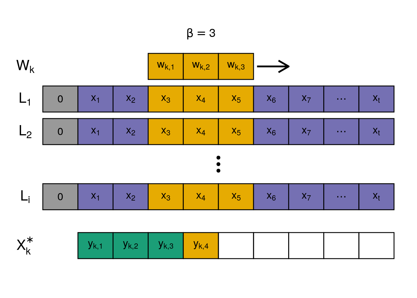
Figure 1.1: Scheme of a 1D convolution operation for a specific kernel k with width \(\beta = 3\). Yellow squares indicate the current convolution at \(t=4\).
| Version | Author | Date |
|---|---|---|
| de8ce5a | Darius Görgen | 2021-04-05 |
Figure 1.1 is an exemplary convolution operation for a specific kernel \(k\) with the kernel width \(\beta=3\). The input matrix \(X\) consists of \(L_i\) individual predictors with \(t\) time steps. The computation of the output involves sliding the kernel window \(W_k\) along the time axis. At the edges of the time series, there is not enough data for the convolution operation. One way to overcome this limitation is called zero-padding. A value of 0 is assumed for unavailable data, indicated by the gray boxes on the left. Another method, which would eventually alter the size of the time axis, is to simply drop the observations for which no calculation with the kernel width \(\beta\) is possible. This behavior is leveraged in many applications to effectively reduce the size of the data sequence at higher abstraction levels within the network, e.g., in applications of CNNs in image recognition (Krizhevsky et al., 2017). The individual outputs \(y_{k,t}\) are obtained by summing up the products of the inputs and the weights within the kernel window, indicated by the yellow boxes. The weights of \(W_k\) remain the same for one kernel but not across different kernels. Note that the result of the operation was denoted \(X^*_k\) to indicate it is an intermediate output, so one does not confuse it with the final network output \(\hat{Y}\). Convolutional layers rarely represent the final layer in a network. It is prevalent to stack multiple convolutional layers on top of each other so that the outputs of the first are used as the inputs to the next (Rawat and Wang, 2017). For this reason, a given 1D convolutional layer at position \(l\) within the network and an input \(X^{l-1}\) is defined by Equation (1.9),
\[\begin{equation} X^l_\beta = \sigma \Big( \sum\limits^L_{i=1} X^{l-1}_i \cdot k^l_{i\beta} + b^l_{i\beta} \Big) \tag{1.9} \end{equation}\]
where \(k\) is the number of kernels, \(\beta\) indicates the size of the filter kernels, \(L\) is the number of input features in \(X^{l-1}\), the bias is represented with \(b\), \(\sigma\) is an activation function and \((\cdot)\) represents the convolutional operation explained in Figure 1.1. In practice, convolutional layers are often combined with so-called pooling layers, which combine the advantages of further reducing the dimensionality of the inputs and extracting latent patterns in the data (Rawat and Wang, 2017). The pooling layers exist in two favors, namely average and maximum pooling. It requires the specification of a pooling window, like the kernel window in the convolutional layer, which will then be applied over the input data to generate the average or maximum value of the observation window. A difference to the convolution kernel is that the pooling will be applied to each kernel individually and that most commonly, the pooling windows will be non-overlapping. Again, by using a zero-padding strategy, the shortening of the time series can be averted.
1.4 Long Short-Term Memory Network.
The basic building block of LSTMs is recurrency. In deep learning, this is implemented by a simple recurrent cell which is defined by Equation (1.10).
\[\begin{equation} Y_t = h_t; h_t = \sigma \Big( W_h h_{t-1} + W_xX_t + b \Big) \tag{1.10} \end{equation}\]
Here, the recurrent information, also referred to as hidden state, \(h_t\) is defined by the previous hidden state \(h_{t-1}\), the current input \(X_t\) and the associated learnable weights \(W_{h}\), \(W_x\) and the bias \(b\). \(\sigma\) is an activation function. That way, recurrent networks have information from earlier time steps available when \(X_t\) is processed. However, long-term dependencies in the input sequence are not very well captured by this simple recurrent cell because of the exploding or vanishing gradient problem (Yu et al., 2019). To capture long-term dependencies in the data, Hochreiter and Schmidhuber (1997) proposed an extension to the simple recurrent cell referred to as Long Short-Term Memory cell, which was later modified to today’s most common LSTM architecture by Gers et al. (2000).
knitr::include_graphics("./assets/img/LSTM.png")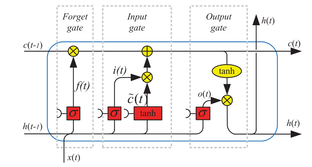
Figure 1.2: Scheme of a Long Short-Term Memory cell. (Source: Yu et al. (2019))
Figure 1.2 depicts the inner structure of a LSTM cell. The input data flows from left to right. There are two inputs to the cell, namely the inputs \(x_t\) as well as \(h_{t-1}\), similar to the basic recurrent cell. The difference is found within the LSTM cell, where red boxes represent so-called gates which are functions with trainable parameters controlling the information flow inside the cell. The cell state \(c_{t-1}\) moves from left to right on the top of the box. At the first intersection, the cell state is updated by a point-wise multiplication with the result of \(\sigma(h_{t-1}x_t)\), which is either 0 or 1 for specific locations. This gate governs which parts of the cell state are set to 0, which is why one refers to it as the forget gate \(f(t)\). The second gate is slightly more complex. First, another variant with individual weights of \(\sigma(h_{t-1}x_t)\) is calculated. Then a point-wise multiplication with \(\widetilde{c}(x_t)\) determines which new information is added linearly to the cell state. Because new information is added to the cell state, this gate is referred to as the input gate. At the final gate, referred to as the output gate \(o(t)\), another multiplicative interaction with the updated cell state and the input determines the cell output \(h_t\). Additionally, the new cell state \(c_t\) is an output, both of which will be used in the next step of an unfolded LSTM to process the input at \(x_{t+1}\). Mathematically, such an LSTM cell is defined by the following equations:
\[\begin{equation} \begin{aligned} & f(t) = \sigma (W_{fh} h_{t-1} + W_{fx}x_t + b_f), \\ & i(t) = \sigma (W_{ih} h_{t-1} + W_{ix}x_t + b_i), \\ & \widetilde{c}(t) = tanh(W_{\widetilde{c}h} h_{t-1} + W_{\widetilde{c}x}x_t + b_{\widetilde{c}}), \\ & c(t) = f(t) \cdot c_{t-1} + i(t) \cdot \widetilde{c}_t, \\ & o(t) = \sigma (W_{oh} h_{t-1} + W_{ox}x_t + b_0), \\ & h_t = o_t \cdot tanh(c_t). \end{aligned} \tag{1.11} \end{equation}\]
A common regularization strategy to reduce the tendency to overfit the training data is to include dropout layers after an LSTM layer. The dropout layer randomly silences a specific percentage of the neurons in a LSTM, thus directing each neuron’s learning process towards learning more general features in the input sequence. Also, multiple LSTM layers can be stacked on top of each other, similar to CNNs, so that the first layer’s output will be used as the input to the next. LSTMs have been reported to achieve considerable results in various problem fields for their capacity to capture both long and short-term dependencies. Researchers from Google achieved a high accuracy by using a LSTM in a sequence-to-sequence problem in machine translation (Wu et al., 2016). Other use cases are the prediction of stream flows in rivers (Hu et al., 2020), estimates of monthly rainfall (Chhetri et al., 2020), or predicting the occurrences of armed conflict in India (Hao et al., 2020).
1.5 Model architecture.
The proposed model leverages both CNNs and LSTMs by combining them in a multi-input model. CNNs are used at the top of the model in order to yield representative feature map encodings of the high-dimensional conditions of a district and its spatial neighborhood. There are four parallel branches in the network for the model to pick up differences between a district and its buffer zones. Each of these branches processes the available predictors for the respective zone, i.e., the district or its buffers. Figure 1.3 shows one such branch as an example for the network architecture. Note that all four branches follow the same concept but that the specific architecture, i.e., the number of layers and neurons is determined during a hyperparameter optimization explained in the following section.
The first component of a branch consists of a 1D-CNN based on zero-padding that a second CNN layer can follow before the signal goes through a local pooling layer that averages or maximizes a sequence based on a temporal window determined by the pool size. Note that because the network is fed with variable-length input sequences, explained in detail in Section 1.8, a global pooling operation is necessary before the LSTM layers. For equal length input sequences, a flattening layer is typically used to flatten the time sequence to one dimension. With variable-length inputs, this would result in different output sizes, which the LSTM layers could not process. Thus, the global pooling layer reduces the input sequences to the number of kernels in the previous layer. This reduction is then repeated \(h\) times according to the desired prediction horizon and fed into a sequence of a maximum of three LSTM layers coupled with individual dropout layers.
Because this general network structure is applied to a total of four different inputs, the network will produce four distinct sequences. These sequences represent what the network has learned from the input data for each of the buffer zones. They are concatenated and put through a small, fully connected model with three layers to retrieve a single output. Each of these layers shares the same activation function and number of neurons. Since each neuron is fully connected to every neuron in the next layer, this part of the model is referred to as a fully connected model. Figure 1.4 shows the model structure from the concatenation of the four input sequences to the final output. The final layer only has one neuron but is time distributed so that it outputs a single value for every time step in the prediction horizon, which is set here to 12 months. For its activation function, it must output values between 0 and 1 so that it can be interpreted as a probability for the occurrence of conflict, which can be mapped to a specific prediction following Equation (1.2).
cnn <- tibble(x = c(5, 5, 5, 5, 5) ,
              y = c(10, 9, 8, 7, 6),
              text = c("**1-D CNN Layer**",
                       "**1-D CNN Layer**",
                       "**Local Pooling**",
                       "**Global Pooling**",
                       "**Repeat Layer**"),
              specs = c(TeX("$number \\, of \\, kernels: \\; k_1 \\; kernel width: \\; \\beta_1 \\; activation: \\; a_1$"),
                        TeX("$number \\, of \\, kernels: \\; k_2 \\; kernel width: \\; \\beta_2 \\; activation: \\; a_2$"),
                        TeX("$pooling \\, operation: \\; pool_1  \\; pool size:    \\; pool-size$"),
                        TeX("$pooling \\, operation: \\; pool_2$"),
                        TeX("$number \\, of \\, repeats: \\; h = 12$")),
              group = as.factor(c(1, 2, 1, 1, 1)) # 1: mandatory, 2: possible
)
arrows_cnn <- tibble(x = c(5,5,5,5),
                     y = c(9.7, 8.7, 7.7, 6.7),
                     xend = c(5,5,5,5),
                     yend = c(9.4, 8.4, 7.4, 6.4)
)

lstm <- tibble(x = c(5,5,5,5,5,5),
               y = c(5,4,3,2,1,0),
               text = c(
                 "**LSTM Layer**",
                 "**Dropout**",
                 "**LSTM Layer**",
                 "**Dropout**",
                 "**LSTM Layer**",
                 "**Dropout**"),
               specs = c(
                 TeX("number of neurons: $n_1$"),
                 TeX("dropout rate: $d_1$"),
                 TeX("number of neurons: $n_2$"),
                 TeX("dropout rate: $d_2$"),
                 TeX("number of neurons: $n_3$"),
                 TeX("dropout rate: $d_3$")),
               group = as.factor(c(1,1,2,2,2,2))
)

arrows_lstm <- tibble(x = c(5,5,5,5,5,5),
                      y = c(5.7, 4.7, 3.7, 2.7, 1.7, 0.7),
                      xend = c(5,5,5,5,5,5),
                      yend = c(5.4, 4.4, 3.4, 2.4, 1.4, 0.4)
)


ggplot()+
  geom_rect(data = cnn, aes(xmin=x-2, xmax=x+2, ymin=y-.25, ymax=y+.35, linetype=group),
            fill=NA, show.legend = F, color = "black") +
  geom_richtext(data=cnn, aes(x=x,y=y+.18,label=text),  fill = NA, label.color = NA) +
  geom_text(data=cnn, aes(x=x,y=y-.1,label=specs), size=3, parse = T) +
  geom_segment(data=arrows_cnn, aes(x=x,y=y,xend=xend,yend=yend),
               arrow = arrow(length=unit(0.3,"cm")), size = 1) +
  geom_rect(data = lstm, aes(xmin=x-2, xmax=x+2, ymin=y-.25, ymax=y+.35, linetype=group),
            fill=NA, show.legend = F, color = "black") +
  geom_richtext(data=lstm, aes(x=x,y=y+.18,label=text),  fill = NA, label.color = NA) +
  geom_text(data=lstm, aes(x=x,y=y-.1,label=specs), size=3, parse = T) +
  geom_segment(data=arrows_lstm, aes(x=x,y=y,xend=xend,yend=yend),
               arrow = arrow(length=unit(0.3,"cm")), size = 1) +
  theme_classic() +
  labs(x=NULL, y=NULL)+
  theme(line = element_blank(),
        text = element_blank())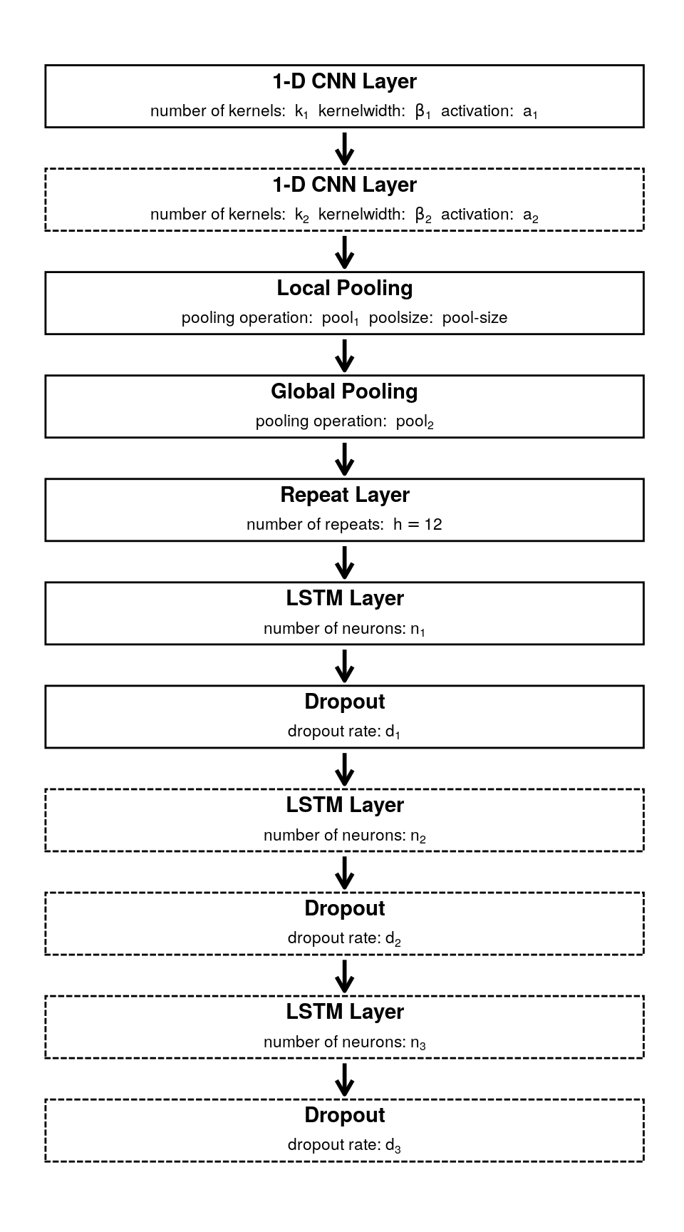
Figure 1.3: Proposed architecture of a single CNN-LSTM branch. Bold lines indicate mandatory layers, dashed lines indicate potential layers which are determined together with other parameters during a hyperparamter optimization process.
| Version | Author | Date |
|---|---|---|
| de8ce5a | Darius Görgen | 2021-04-05 |
fc <- tibble(x = c(5, 5, 5, 5, 5) ,
             y = c(10, 9, 8, 7, 6),
             text = c("**Concatentation Layer**",
                      "**Fully Connected Dense Layer**",
                      "**Fully Connected Dense Layer**",
                      "**Fully Connected Dense Layer**",
                      "**Time Distributed Dense Layer**"),
             specs = c(TeX("$number\\,of\\,input\\,sequences:\\;4$"),
                       TeX("$number\\,of\\,neurons:  \\; n_{dense}  \\; \\; activation:  \\; a_{dense}$"),
                       TeX("$number\\,of\\,neurons:  \\; n_{dense}  \\; \\; activation:  \\; a_{dense}$"),
                       TeX("$number\\,of\\,neurons:  \\; n_{dense}  \\; \\; activation:  \\; a_{dense}$"),
                       TeX("$number\\,of\\,neurons:  \\; 1   \\;\\; activation:  \\; a_{out}  \\; bias \\, initialization: \\; \\pi$")),
             group = as.factor(c(1, 1, 1, 1, 1)) # 1: mandatory, 2: possible
)

arrows_fc <- tibble(x = c(5,5,5,5),
                    y = c(9.7, 8.7, 7.7, 6.7),
                    xend = c(5,5,5,5),
                    yend = c(9.4, 8.4, 7.4, 6.4)
)

ggplot()+
  geom_rect(data = fc, aes(xmin=x-2, xmax=x+2, ymin=y-.25, ymax=y+.35, linetype=group),
            fill=NA, show.legend = F, color = "black") +
  geom_richtext(data=fc, aes(x=x,y=y+.18,label=text),  fill = NA, label.color = NA) +
  geom_text(data=fc, aes(x=x,y=y-.1,label=specs), size=3, parse = T) +
  geom_segment(data=arrows_fc, aes(x=x,y=y,xend=xend,yend=yend),
               arrow = arrow(length=unit(0.3,"cm")), size = 1) +
  theme_classic() +
  labs(x=NULL, y=NULL)+
  theme(line = element_blank(),
        text = element_blank())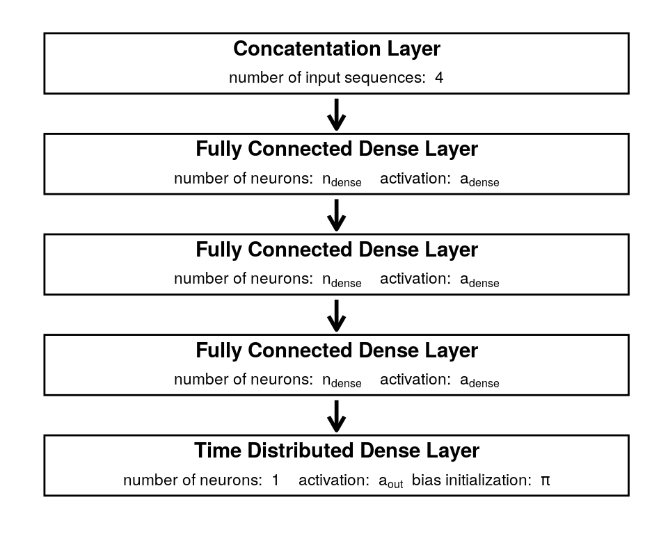
Figure 1.4: Proposed architechture of the fully connected output model.
| Version | Author | Date |
|---|---|---|
| de8ce5a | Darius Görgen | 2021-04-05 |
As mentioned before, the outcome variable is characterized by a very high class imbalance (Table ??). In traditional approaches, researchers have counterbalanced this fact by artificially altering the distribution during training (Halkia et al., 2020; Schellens and Belyazid, 2020). Using downsampling approaches, however, means that there is a reduction in available training data. Because of the relatively short available sequences and a low number of observations, downsampling was not conducted when training the neural network. Instead, a specialized loss function was used to differentiate between easy-to-learn examples, referred to as the background class, and hard-to-classify examples also called foreground class. This function is called focal loss and was initially designed to detect rare objects in image segmentation tasks (Lin et al., 2018). As indicated, the focal loss down-weights the contribution of easy-to-classify examples to the overall loss, thus directing the training process towards optimizing for hard-to-classify examples. It is defined mathematically by Equation (1.12)
\[\begin{equation} \begin{aligned} & p_t = \begin{cases} p & \text{if } y = 1 \\ 1-p & \text{otherwise} \end{cases} \\ & FL(p_t) = -\alpha(1-p_t)^{\gamma} \, log(p_t) , \end{aligned} \tag{1.12} \end{equation}\]
where \(p\) is the probability estimation for an observation outputted by the model, \(\alpha\) is a weighting factor that attributes different weights to the background and foreground class and \(\gamma\) is a parameter governing the magnitude with which easy examples are down-weighted. The original authors state that this loss function has two beneficial properties for contexts with high class imbalance. The first is that for an observation wrongly classified as the background class, while \(p_t\) is small, the loss remains nearly unaffected because the modulating factor \((1-p_t)^{\gamma}\) tends towards 1. However, when \(p_t\rightarrow1\), the term goes towards 0, which means that the contribution of well-classified examples is weighted down. The second property is that the focusing parameter \(\gamma\) leans itself to adjusting the rate at which easy examples are down-weighted based on the problem at hand. When \(\gamma = 0\), the loss is equal to cross-entropy loss, i.e., all examples contribute equally to the overall loss. Both \(\alpha\) and \(\gamma\) are parameters that are optimized during the hyperparameters optimization stage. Additionally, the authors initiate the final output layer with a small value \(\pi\), effectively reducing the probability the network will estimate the occurrence of the foreground class during the early stages of training. They report that this has positive impacts on training stability in high class imbalance scenarios (Lin et al., 2018). This initialization bias is also determined during the optimization stage.
1.6 Bayesian Hyperparameter Optimization
Hyperparameters are not directly involved in predicting a particular output, so they are often contrasted with model parameters. They substantially influence the overall training process and the accuracy of the predictions (Albahli et al., 2020). Table 1.1 summaries the notation of hyperparameters and the associated value ranges. Note that the branch-specific hyperparameters will be optimized for the four different branches in the network corresponding to the districts and the three buffer zones. Various strategies to apply hyperparameter optimization exist. Among the most widely used are grid search, random search, Bayesian Optimization (BO), and more recently the training of machine-learning models to predict the accuracy of different model configurations, also called meta-learning (Baik et al., 2020; Yu and Zhu, 2020).
hyperparas <- tibble(name = c("lstm\\_layers",
                              "double\\_cnn",
                              "a_{cnn}",
                              "k_{cnn}",
                              "\\beta_{cnn}",
                              "pool_1",
                              "pool\\_size",
                              "pool_2",
                              "n_{1}",
                              "d_{1}",
                              "n_{2}",
                              "d_{2}",
                              "n_{3}",
                              "d_{3}",
                              "a_{dense}",
                              "n_{dense}",
                              "a_{out}",
                              "\\pi",
                              "\\alpha",
                              "\\gamma",
                              "opti",
                              "lr"),
                     descr = c("Number of LSTM Layers",
                               "Use of a second CNN layer",
                               "Activation function for CNN layers",
                               "Number of kernels in CNN layers",
                               "Kernel width for CNN layers",
                               "Pooling operation for local pooling",
                               "Pool size for local pooling",
                               "Pooling operation for global pooling",
                               "Number of neurons in first LSTM layer",
                               "Rate of dropout in first LSTM layer",
                               "Number of neurons in second LSTM layer",
                               "Rate of dropout in second LSTM layer",
                               "Number of neurons in third LSTM layer",
                               "Rate of dropout in third LSTM layer",
                               "Activation of the dense model",
                               "Neurons per layer in the dense model",
                               "Activation of the output layer",
                               "Value of bias initialization of output layer",
                               "Alpha parameter of focal loss function",
                               "Gamma parameter of focal loss function",
                               "Optimizer function",
                               "Learning rate of the optimizer function"),
                     values = c("1-3",
                                "Yes, No",
                                "sigmoid, hard\\_sigmoid, softmax,\\\\softplus, softsign",
                                "12-128",
                                "3-24",
                                "maximum, average",
                                "3-24",
                                "maximum, average",
                                "12-128",
                                "0-0.5",
                                "12-128",
                                "0-0.5",
                                "12-128",
                                "0-0.5",
                                "sigmoid, hard\\_sigmoid, softmax,\\\\softplus, softsign, relu,\\\\elu, selu, tanh",
                                "12-128",
                                "sigmoid, hard\\_sigmoid, softmax",
                                "0-1",
                                "0-1",
                                "0-10",
                                "rmsprop, adam, adadelta,\\\\adagrad, adamax, sgd",
                                "1^{-10} - 1"))

hyperparas$name = paste("$", hyperparas$name, "$", sep = "")
hyperparas$values = paste("$", hyperparas$values, "$", sep = "")

hyperparas %>%
  rename(Name = name, Description = descr, 'Value Ranges' = values) %>%
  thesis_kable(linesep = c(""),
        align = "lll",
        caption = c("Overview of model hyperparameters."),
        escape = F,
        longtable = T) %>%
  kable_styling(latex_options = c("HOLD_position", "repeat_header"),
                font_size = 10) %>%
  group_rows("Branch specific hyperparameters", 1, 14) %>%
  group_rows("Global hyperparameters", 15, 22) %>%
  footnote(general = "Branch specific parameters are optimized individually for the 0/50/100/200 km input branches. Global parameters are optimized once per model.",
           threeparttable = T,
           escape = FALSE,
           general_title = "General:",
footnote_as_chunk = T)| Name | Description | Value Ranges |
|---|---|---|
| Branch specific hyperparameters | ||
| \(lstm\_layers\) | Number of LSTM Layers | \(1-3\) |
| \(double\_cnn\) | Use of a second CNN layer | \(Yes, No\) |
| \(a_{cnn}\) | Activation function for CNN layers | \(sigmoid, hard\_sigmoid, softmax,\\softplus, softsign\) |
| \(k_{cnn}\) | Number of kernels in CNN layers | \(12-128\) |
| \(\beta_{cnn}\) | Kernel width for CNN layers | \(3-24\) |
| \(pool_1\) | Pooling operation for local pooling | \(maximum, average\) |
| \(pool\_size\) | Pool size for local pooling | \(3-24\) |
| \(pool_2\) | Pooling operation for global pooling | \(maximum, average\) |
| \(n_{1}\) | Number of neurons in first LSTM layer | \(12-128\) |
| \(d_{1}\) | Rate of dropout in first LSTM layer | \(0-0.5\) |
| \(n_{2}\) | Number of neurons in second LSTM layer | \(12-128\) |
| \(d_{2}\) | Rate of dropout in second LSTM layer | \(0-0.5\) |
| \(n_{3}\) | Number of neurons in third LSTM layer | \(12-128\) |
| \(d_{3}\) | Rate of dropout in third LSTM layer | \(0-0.5\) |
| Global hyperparameters | ||
| \(a_{dense}\) | Activation of the dense model | \(sigmoid, hard\_sigmoid, softmax,\\softplus, softsign, relu,\\elu, selu, tanh\) |
| \(n_{dense}\) | Neurons per layer in the dense model | \(12-128\) |
| \(a_{out}\) | Activation of the output layer | \(sigmoid, hard\_sigmoid, softmax\) |
| \(\pi\) | Value of bias initialization of output layer | \(0-1\) |
| \(\alpha\) | Alpha parameter of focal loss function | \(0-1\) |
| \(\gamma\) | Gamma parameter of focal loss function | \(0-10\) |
| \(opti\) | Optimizer function | \(rmsprop, adam, adadelta,\\adagrad, adamax, sgd\) |
| \(lr\) | Learning rate of the optimizer function | \(1^{-10} - 1\) |
| General: Branch specific parameters are optimized individually for the 0/50/100/200 km input branches. Global parameters are optimized once per model. | ||
Different approaches have in common what Shahriari et al. (2016) called “taking the human out of the loop.” Hyperparameter tuning in this way can be understood as a process of reducing the impact of a researcher’s subjectivity on the model construction towards the machine and the data controlling the training process. In its most extreme form, this thought leads towards machines being able to determine how they can learn a specific problem by themselves (Yao et al., 2019). The approaches, however, differ in complexity and the way they cope with the problem to balance between search time and accuracy. For example, grid search might yield equally high accuracies but the training time needed to achieve these can be very high compared with BO (Wu et al., 2019). While the meta-learning approach certainly is beyond this thesis’s scope, an optimization strategy was searched with a reasonable balance between computing efficiency in terms of time and high accuracy. The choice was made to apply BO because it explicitly leverages prior information on the performance of hyperparameters to determine the next set to be explored and has a proven record of delivering robust results since its original publication in the 1970s (Mockus et al., 2014). In essence, BO works by iteratively updating the beliefs on the distribution of an accuracy metric for an objective function \(f\) based on the knowledge of prior samples of parameter \(x\). The goal is to find the global maximum for \(x^+\) within a pre-defined search space \(A\) following Equation (1.13)
\[\begin{equation} x^+ = arg\;\underset{x \in A}{max} \, f(x). \tag{1.13} \end{equation}\]
This is achieved by updating the prior probability \(P(f(x))\) given data \(D\) to get the posterior probability \(P(f(x)|D)\), which is referred to as the Bayes’ theorem (Bayes and Price, 1763). Assume that we have accumulated a dataset \(D_{1:t-1} = [(x_1,y_1) \dots (x_{t-1},y_{t-1})]\) where \(x_1\) is the value of a hyperparameter at trial \(t = 1\) and \(y_1\) is the result of the objective function \(y_1 = f(x_1)\) which, in the case at hand, is the performance of the proposed model measured by a specific accuracy metric. This knowledge data can be queried by an acquisition function \(u\) to retrieve the next promising candidate \(x_t\) following Equation (1.14)
\[\begin{equation} x_{t} = arg \;\underset{x}{max} \, u(x|D_{1:t-1}) \tag{1.14} \end{equation}\]
With this candidate at hand the model is retrained to obtain an additional measurement on the performance. The knowledge data set is updated by \(D_{1:t} = \{D_{1:t-1},(x_t,y_t)\}\) and a new posterior probability for \(f(x)\) can be estimated. BO works by calculating the probability density function for a given parameter \(x\) based on a Gaussian process. The details of these calculations are beyond this thesis’s scope, but the reader is referred to Rasmussen and Williams (2006) for a comprehensive analysis of its application in machine learning. As an acquisition function, the Upper Confidence Bound (UCB) function was used to calculate the next candidate parameter \(x_t\). For a comprehensive overview of a BO process using UCB be referred to (Srinivas et al., 2012). It should be noted that BO, in its essence, is a sequential problem because the results of one iteration will impact the next. Even though there have been efforts to parallelize BO (Nomura, 2020), these approaches do not alter the basic sequential characteristic of the algorithm and come with higher management costs for the researcher.
1.7 Performance Metrics
The performance of a model is validated on a specific set of accuracy metrics. However, performance is often a multi-dimensional problem, which is why several metrics are used in this thesis. These were selected to represent different dimensions of a model’s performance to differentiate between the occurrence of conflicts versus peace.
In its essence, the problem of this thesis is one of a binary classification. The core component for the performance assessment of a binary classification problem is a simple two-class confusion matrix depicted in Table 1.2 (Tharwat, 2020).
cnf <- tibble(col1 = c("", "*Positives*", "*Negatives*"),
              col2 = c("*Positives*", "True Positives (TP)", "False Negatives (FN)"),
              col3 = c("*Negatives*", "False Positives (FP)", "True Negatives (TN)"))

thesis_kable(cnf,
      col.names = c("","", ""),
      align = "ccc",
      escape = F,
      caption = "Concept of a binary confusion matrix.") %>%
  kable_styling(latex_options = c("HOLD_position", "repeat_header"),
                font_size = 10) %>%
  add_header_above(c("", "Observation" = 2), bold = T) %>%
group_rows("Prediction", 2,3)| Positives | Negatives | |
| Prediction | ||
| Positives | True Positives (TP) | False Positives (FP) |
| Negatives | False Negatives (FN) | True Negatives (TN) |
From the table above, it is evident that there are two types of errors. False Positives (FP), also referred to as Type I error, are observations that were falsely classified as the positive class while in reality they belong to the negative class. False Negatives (FN), referred to as the Type II error, are observations that were predicted as the negative class, however, they belong to the positive class (Tharwat, 2020). The most widely used accuracy metric derived from a confusion matrix is Overall Accuracy (OA). It is simply calculated as the rate of correctly classified observations (Equation (1.15))
\[\begin{equation} OA = \frac{TP+TN}{TP+TN+FP+FN}\;. \tag{1.15} \end{equation}\]
However, OA is not very well suited for classification problems with high class imbalance (Tharwat, 2020). A model for a classification problem where the positive class only covers 1 % of the observations can achieve an OA of 99 % only by always predicting the negative class. In the context of class imbalance, other metrics derived from the confusion matrix help to paint a more concise picture of a model’s capability to predict a particular outcome. The rate at which positive examples are correctly classified (True Positive Rate), also called sensitivity or recall, sheds light on a models capability to correctly identify positive observations (Equation (1.16))
\[\begin{equation} Sensitivity = TPR = \frac{TP}{TP+FN}\;. \tag{1.16} \end{equation}\]
The False Positive Rate (FPR) contains information on the rate a model falsely predicts a positive outcome in relation to all observations with a negative outcome thus indicating the rate negative observations are treated as positives (Equation (1.17))
\[\begin{equation} FPR = \frac{FP}{FP+TN}\;. \tag{1.17} \end{equation}\]
Shifting the focus towards the negative class, specificity also called True Negative Rate (TNR) describes the rate negative observations are correctly identified (Equation (1.18))
\[\begin{equation} Specificity = TNR = \frac{TN}{TN+FP}\;. \tag{1.18} \end{equation}\]
The False Negative Rate (FNR) then describes the rate that positive observations are falsely classified as the negative class (Equation (1.19))
\[\begin{equation} FNR = \frac{FN}{FN+TP}\;. \tag{1.19} \end{equation}\]
In addition to these metrics, the precision of a model, also referred to as Positive Predictive Value (PPV) captures the rate examples classified as the positive class actually represent positive observations (Equation (1.20))
\[\begin{equation} Precision = PPV = \frac{TP}{TP+FP}\;. \tag{1.20} \end{equation}\]
Note that sensitivity and precision always are in a fragile balance with each other. While higher sensitivity values can be achieved by decreasing the number of false negatives, there naturally will be a higher number of false positives, and the precision is decreased. The same holds if one tries to increase the precision, which will lead to lower sensitivity values. To harmonize this relationship into a single metric the \(F_\beta\)-score is used (Equation (1.21))
\[\begin{equation} F_\beta = (1+\beta^2)\frac{Precision*Sensitivity}{\beta^2*Precision+Sensitivity}\;. \tag{1.21} \end{equation}\]
The most widely used is \(\beta = 1\), which will result in a harmonic mean between precision and sensitivity, also referred to as \(F_1\)-score (Tharwat, 2020). With increasing values of \(\beta\), sensitivity is emphasized over precision. \(\beta=2\) will put the double weight of sensitivity compared to precision. This metric, referred to as \(F_2\)-score, is the central metric for this thesis. It was chosen because a model’s capability to not miss out on the occurrence of conflict district-months was considered more important than a model’s tendency towards so-called false alarms, i.e., the prediction of conflict when in reality, there was peace. If this model was used in conflict prevention or crisis early warning systems, missing out on a potential conflict can lead to the loss of lives. It is therefore considered advantageous when a model can correctly detect positive examples at a high rate. However, using the \(F_2\)-score as the central optimization metric ensures that the precision of a model still influences its performance evaluation so that frequently predicting the positive class itself would not lead to very high performance scores.
Two additional metrics which can not directly be derived from the confusion matrix are included as well. These are the Area Under the Receiver Operating Characteristic (AUROC - AUC for short) as well as the Area Under the Precision-Recall Curve (AUPRC - AUPR for short) (Fawcett, 2006). These metrics represent the relative tradeoffs between sensitivity and FPR, and precision and sensitivity, respectively. To get an intuition about the calculation, one can imagine that the threshold value to map a model’s output to a specific class prediction steadily increases from 0 to 1. In the former case, for each threshold, the values for sensitivity and FPR are recorded. In the latter case, precision and sensitivity are the metrics of interest. In reality, a more efficient algorithm is used to calculate these metrics (Fawcett, 2006). Both metrics are then plotted against each other. The area under theses curves generalizes the performance of a classifier into a single metric. The generated plots of both the ROC and the PRC, can be used to compare the performance of different classifiers visually (Fawcett, 2006).
1.8 Training & Validation Process
Recall that the training data is available as a sequence of \(L\) predictors of \(t\) time steps in the form of \(X^L_t\) from Equation (1.3). In total, there are \(t = 228\) time steps available from January 2001 to December 2019. The total number of predictors is \(L = 176\), but only a subset is fed to the respective models, except for the regression baseline and the environmental models which are trained on the complete data set. The prediction horizon is set to 12 months so that for each \(x_t\) there is an associated outcome vector of the form \(y = [{y_{t+1},y_{t+2},...,y_{t+12}}]\).
In order to be able to evaluate the potential of a model to generalize, out-of-sample evaluation data sets are needed. The available data is split into three different sets, which are used for training, validation, and testing according to Table 1.3.
data_sets <- tibble(Name = c("Training",
                             "Validation",
                             "Test"),
                    Purpose = c("Fit model parameters",
                                "Fit model hyperparameters",
                                "Performance estimation"),
                    'Range' = c("Jan. 2001 - Dec. 2016",
                                "Jan. 2017 - Dec. 2018",
                                "Jan. 2019 - Dec. 2019"))

thesis_kable(data_sets,
      align = "lll",
      caption = "Split of the available data to training, validation and testing data sets.",
      escape = F,
      longtable = T) %>%
  kable_styling(latex_options = c("HOLD_position"),
font_size = 10)| Name | Purpose | Range |
|---|---|---|
| Training | Fit model parameters | Jan. 2001 - Dec. 2016 |
| Validation | Fit model hyperparameters | Jan. 2017 - Dec. 2018 |
| Test | Performance estimation | Jan. 2019 - Dec. 2019 |
For the LR baseline, all available predictors are used. Because no hyperparameter tuning is involved in fitting the model, the training and validation data sets are combined to estimate the model parameters. Undersampling is performed so that an equal amount of observations with conflict and peace district-months is included. While all conflict observations are included, peace observations are randomly sampled. This process is repeated ten times, each with different selected peace observations. For each month in the prediction horizon, models are trained individually. Time is not included as a predictor variable, so that the model predictions e.g. for six month into the future are based solely on the predictors at time step \(t\): \(\hat{y}_{t+6} = f(x_t)\). The predictor variables are normalized based on the distribution in the combined training and validation set. District-months with missing data are dropped for the logistic regression model. Threshold tuning on the model’s probability predictions is applied in the sense that the threshold is chosen which delivers the best \(F_2\)-score on the training data. With this threshold, the performance metrics are evaluated on the test set and averaged across the ten repeats. The average of the monthly performance metrics is calculated and referred to as the global performance.
Handling the data for training the neural networks differs considerably compared to the LR baseline. For all neural network models, the data is handed over as a time series with increasing length and a minimum length of 48 months. Batch gradient descent was chosen as a training strategy, meaning that the first step in an epoch of training a neural network consists of 48 months worth of data for all the districts. Then gradients are calculated, and the learnable model parameters are updated. The next step in an epoch then consists of training data worth of \(t = 48\, months + step\_size\) time steps for all available districts. During hyperparameter optimization, a \(step\_size = 4\) was chosen, effectively reducing the size of the training data set to \(\frac{1}{4}\). During the models’ final training, \(step\_size=1\) was chosen so that the complete data set is used to estimate the final model parameters. One epoch of training is completed once all time steps have been presented to the model. Performance on the validation set is calculated at the end of an epoch. A global termination criterion for training is implemented for all models, once 200 epochs have been trained. This is combined with different early stopping policies for the optimization and the final training stage, which will lead to varying numbers of epochs from one model to another. Similar to the logistic regression model, the predictor variables are normalized based on the distribution in the training data set. Missing values, in contrast, are not dropped but imputed with a value of -1. Due to normalization, valid values are in the range of \([0,1]\), so replacing missing data with a constant value represents a valid training strategy for deep learning frameworks (Ipsen et al., 2020). Also, missing values mainly occurred systematically in the present data set. For example, values of evapotranspiration are systematically missing for the Sahara region. Other imputation strategies, such as mean imputation of interpolation between the last and next observed value in a time series, cannot deliver robust results in such cases. Also, a comparable pattern of missingness is expected in the test set, and missing values are expected to occur not in relation to the outcome variable but due to the characteristics governing their respective generating process.
Hyperparameter optimization for the neural networks is performed only once with the outcome variable cb to minimize computation time. Even though it can be expected that the optimal configurations of the network architecture might differ for the outcome variables, this simplification drastically reduces training time. Additionally, the internal structure of the data does not change with the outcome variable, so that it can be expected that this one-to-serve-all approach will lead to satisfactory performance with other outcome variables. For both aggregation units, adm and bas, and the different predictor sets (CH, SV, EV) optimization is conducted individually, resulting in a total number of six optimization processes. For one optimization process, the first 100 trials are conducted with random initialization of the hyperparameters. These first trials serve as the knowledge base to estimate the performance of yet-to-be-tested parameters. Another iteration of 100 trials are then used to explore and optimize the parameter space. During this stage, the training set is used to optimize model parameters. The \(F_2\)-score is evaluated on the validation data set at the end of each epoch. During training, threshold tuning is not applied, which is why \(\lambda = 0.5\) is used as the cut-off value to calculate the \(F_2\)-score. Early stopping was included when the \(F_2\)-score on the validation data set does not improve for ten epochs above a threshold of \(0.001\).
The final training process is conducted for each predictor set on each of the four outcome variables for both aggregation units. The model is set up with the optimal hyperparameters found during the optimization stage. There are two steps involved in the final training stage. The first step consists of training the model parameters on the training set with a slightly changed early stopping policy on evaluating the validation set. Here, training is stopped after 20 epochs of no improvement in the \(F_2\)-score above a threshold of \(0.0001\). The policy is slightly changed because firstly, more training data is available, and secondly, the hyperparameters have been optimized for the response variable cb only. To account for possible variations during training, the stopping criterion is relaxed so that a higher number of training epochs are possible. Once training has been completed, threshold tuning is applied based on the validation data set to find the threshold which optimizes the \(F_2\)-score. During the second step, the model parameters are trained on the validation set, which has been held out during the first step. Because there is no other independent data set to validate this training process against, the early stopping criterion is set to a decrease in the overall loss smaller than 0.0001 within 10 epochs. After the second training step, the model performance is evaluated on the test set. For this, the model’s estimation for the probability of conflict is predicted, then the optimized threshold from the first training step is applied, and the performance metrics are recorded. Because the weights of different layers are randomly initialized, the prediction results can substantially differ when training is repeated. To account for this variability, training is repeated 10 times on each predictor set for both aggregation units and all outcome variables, resulting in a total number of 240 distinct DL models (10 repeats x 4 outcome classes x 3 predictor sets x 2 aggregation units).
1.9 Analysis of Variance
Leveraging the availability of ten repeats per outcome variable and predictor set a two-way analysis of variance (ANOVA) is used to derive statistical indications to answer hypothesis H1 and H2. ANOVA is used to analyze the impact of different treatment factors on the outcome of an experiment. The four different model and predictor themes (LR, CH, SV, and EV) in combination with the spatial representation (adm and bas) are conceptualized as two different levels of treatment. The outcome of the experiment is measured by the achieved global \(F_2\)-score. Three assumptions must hold for the classical Fisher’s ANOVA (Fisher, 1921). The first is the independence of observations between and within groups of treatment. This independence is given since the results of one predictor set do not impact the results of another. The ten repeats of the DL models for a given predictor-unit combination are independent from each other because instead of a cross-validation the total available data set is used for each repeat (Raschka, 2020). For the LR model, downsampling is conducted randomly so that for each repeat peace observations have the same probability to be included during training. The second assumption is that residuals are normally distributed and thirdly homogeneity of variance is assumed. Visualizations of the residuals are used to assess if the assumptions are violated. While the assumption of normal distribution holds (Figure ??), the assumptions on homogeneous variance is slightly violated (Figure ??). For that reason, instead of the classical ANOVA, the Welch-James test is applied (James, 1951; Welch, 1951) which tests for \(H_0\) that no statistical significant difference in the mean of the outcome is observed between treatments. It is a non-parametric test and thus can be applied for cases where variance is not homogeneous. When \(H_0\) can be refused, usually post-hoc tests are applied to investigate the differences between groups. For cases where two or more treatment groups are tested against, the test is specified by terms describing the individual group’s contributions (main effect) as well as the interaction terms between groups (interaction effect). When interaction effects are significant, main effects are excluded from further analysis. The Games-Howell test is applied as a post-hoc test. It can be applied when six or more observations for each group are present (Lee and Lee, 2018). It delivers an estimate of the absolute difference between treatment groups and reports on the statistical significance of these differences. The results thus allow a detailed comparison of the achieved performances for different predictor-unit combinations based on statistical significance and thus play a central role in the confirmation of hypothesis H1 and H2.
2 References
Albahli, S., Alhassan, F., Albattah, W., Khan, R.U., 2020. Handwritten Digit Recognition: Hyperparameters-Based Analysis. Applied Sciences 10, 5988. https://doi.org/10.3390/app10175988
Ali, A., Shamsuddin, S.M., Ralescu, A., 2015. Classification with class imbalance problem: A review. International Journal of Advances in Soft Computing and its Applications 5, 176–204.
Baik, S., Choi, M., Choi, J., Kim, H., Lee, K.M., 2020. Meta-Learning with Adaptive Hyperparameters, in: Larochelle, H., Ranzato, M., Hadsell, R., Balcan, M.F., Lin, H. (Eds.), Advances in Neural Information Processing Systems. pp. 20755–20765.
Bayes, M., Price, M., 1763. An Essay towards Solving a Problem in the Doctrine of Chances. By the Late Rev. Mr. Bayes, F. R. S. Communicated by Mr. Price, in a Letter to John Canton, A. M. F. R. S. Philosophical Transactions (1683-1775) 53, 370–418.
Chhetri, M., Kumar, S., Pratim Roy, P., Kim, B.-G., 2020. Deep BLSTM-GRU Model for Monthly Rainfall Prediction: A Case Study of Simtokha, Bhutan. Remote Sensing 12, 3174. https://doi.org/10.3390/rs12193174
Cordoni, F., 2020. A comparison of modern deep neural network architectures for energy spot price forecasting. Digital Finance 2, 189–210. https://doi.org/10.1007/s42521-020-00022-2
Fawcett, T., 2006. An introduction to ROC analysis. Pattern Recognition Letters, ROC Analysis in Pattern Recognition 27, 861–874. https://doi.org/10.1016/j.patrec.2005.10.010
Fisher, R.A., 1921. Studies in crop variation. I. An examination of the yield of dressed grain from Broadbalk. The Journal of Agricultural Science 11, 107–135. https://doi.org/10.1017/S0021859600003750
Gers, F.A., Schmidhuber, J., Cummins, F., 2000. Learning to forget: Continual prediction with LSTM. Neural Computation 12, 2451–2471. https://doi.org/10.1162/089976600300015015
Halkia, M., Ferri, S., Schellens, M.K., Papazoglou, M., Thomakos, D., 2020. The Global Conflict Risk Index: A quantitative tool for policy support on conflict prevention. Progress in Disaster Science 6, 100069. https://doi.org/10.1016/j.pdisas.2020.100069
Hao, M., Fu, J., Jiang, D., Ding, F., Chen, S., 2020. Simulating the Linkages Between Economy and Armed Conflict in India With a Long Short-Term Memory Algorithm. Risk Analysis 40, 1139–1150. https://doi.org/10.1111/risa.13470
Hegre, H., Allansson, M., Basedau, M., Colaresi, M., Croicu, M., Fjelde, H., Hoyles, F., Hultman, L., Högbladh, S., Jansen, R., Mouhleb, N., Muhammad, S.A., Nilsson, D., Nygård, H.M., Olafsdottir, G., Petrova, K., Randahl, D., Rød, E.G., Schneider, G., von Uexkull, N., Vestby, J., 2019. ViEWS: A political violence early-warning system. Journal of Peace Research 56, 155–174. https://doi.org/10.1177/0022343319823860
Hochreiter, S., Schmidhuber, J., 1997. Long Short-Term Memory. Neural Computation 9, 1735–1780. https://doi.org/10.1162/neco.1997.9.8.1735
Hu, Y., Yan, L., Hang, T., Feng, J., 2020. Stream-Flow Forecasting of Small Rivers Based on LSTM. arXiv:2001.05681 [cs].
Ipsen, N., Mattei, P.-A., Frellsen, J., 2020. How to deal with missing data in supervised deep learning?, in: Art of Learning with MissingValues (Artemiss).
James, G.S., 1951. The Comparison of Several Groups of Observations When the Ratios of the Population Variances are Unknown. Biometrika 38, 324–329. https://doi.org/10.2307/2332578
Krizhevsky, A., Sutskever, I., Hinton, G.E., 2017. ImageNet classification with deep convolutional neural networks. Communications of the ACM 60, 84–90. https://doi.org/10.1145/3065386
Lee, H., Largman, Y., Pham, P., Ng, A.Y., 2009. Unsupervised feature learning for audio classification using convolutional deep belief networks, in: Proceedings of the 22nd International Conference on Neural Information Processing Systems, NIPS’09. Curran Associates Inc., Red Hook, NY, USA, pp. 1096–1104.
Lee, S., Lee, D.K., 2018. What is the proper way to apply the multiple comparison test? Korean Journal of Anesthesiology 71, 353–360. https://doi.org/10.4097/kja.d.18.00242
Li, T., Hua, M., Wu, X., 2020. A Hybrid CNN-LSTM Model for Forecasting Particulate Matter (PM2.5). IEEE Access 8, 26933–26940. https://doi.org/10.1109/ACCESS.2020.2971348
Lin, T.-Y., Goyal, P., Girshick, R., He, K., Doll’ar, P., 2018. Focal Loss for Dense Object Detection. arXiv:1708.02002 [cs].
Mehtab, S., Sen, J., Dasgupta, S., 2020. Robust Analysis of Stock Price Time Series Using CNN and LSTM-Based Deep Learning Models, in: Proceedings of the 4th International Conference on Electronics, Communication and Aerospace Technology (ICECA). IEEE, Coimbatore, pp. 1481–1486. https://doi.org/10.1109/ICECA49313.2020.9297652
Mockus, J., Tiesis, V., Zilinskas, A., 2014. The application of Bayesian methods for seeking the extremum, in: Hey, A.M. (Ed.), Towards Global Optimization 2. pp. 117–129.
Nomura, M., 2020. Simple and Scalable Parallelized Bayesian Optimization. arXiv:2006.13600 [cs, stat].
Parr, T., Howard, J., 2018. The Matrix Calculus You Need For Deep Learning. arXiv:1802.01528 [cs, stat].
Rajagukguk, R.A., Ramadhan, R.A.A., Lee, H.-J., 2020. A Review on Deep Learning Models for Forecasting Time Series Data of Solar Irradiance and Photovoltaic Power. Energies 13, 6623. https://doi.org/10.3390/en13246623
Raschka, S., 2020. Model Evaluation, Model Selection, and Algorithm Selection in Machine Learning. arXiv:1811.12808 [cs, stat].
Rasmussen, C.E., Williams, C.K.I., 2006. Gaussian processes for machine learning, Adaptive computation and machine learning. MIT Press, Cambridge, Massachusetts.
Rawat, W., Wang, Z., 2017. Deep convolutional neural networks for image classification: A comprehensive review. Neural Computation 29, 2352–2449. https://doi.org/10.1162/NECO_a_00990
Schellens, M.K., Belyazid, S., 2020. Revisiting the Contested Role of Natural Resources in Violent Conflict Risk through Machine Learning. Sustainability 12, 6574. https://doi.org/10.3390/su12166574
Shahriari, B., Swersky, K., Wang, Z., Adams, R.P., de Freitas, N., 2016. Taking the Human Out of the Loop: A Review of Bayesian Optimization. Proceedings of the IEEE 104, 148–175. https://doi.org/10.1109/JPROC.2015.2494218
Song, J., Gao, S., Zhu, Y., Ma, C., 2019. A survey of remote sensing image classification based on CNNs. Big Earth Data 3, 232–254. https://doi.org/10.1080/20964471.2019.1657720
Srinivas, N., Krause, A., Kakade, S.M., Seeger, M., 2012. Gaussian Process Optimization in the Bandit Setting: No Regret and Experimental Design. IEEE Transactions on Information Theory 58, 3250–3265. https://doi.org/10.1109/TIT.2011.2182033
Sun, S., Cao, Z., Zhu, H., Zhao, J., 2019. A Survey of Optimization Methods from a Machine Learning Perspective. arXiv:1906.06821 [cs, math, stat].
Tharwat, A., 2020. Classification assessment methods. Applied Computing and Informatics 17. https://doi.org/10.1016/j.aci.2018.08.003
Welch, B.L., 1951. On the Comparison of Several Mean Values: An Alternative Approach. Biometrika 38, 330–336. https://doi.org/10.2307/2332579
Wu, J., Chen, X.-Y., Zhang, H., Xiong, L.-D., Lei, H., Deng, S.-H., 2019. Hyperparameter Optimization for Machine Learning Models Based on Bayesian Optimizationb. Journal of Electronic Science and Technology 17, 26–40. https://doi.org/10.11989/JEST.1674-862X.80904120
Wu, Y., Schuster, M., Chen, Z., Le, Q.V., Norouzi, M., Macherey, W., Krikun, M., Cao, Y., Gao, Q., Macherey, K., Klingner, J., Shah, A., Johnson, M., Liu, X., Kaiser, Gouws, S., Kato, Y., Kudo, T., Kazawa, H., Stevens, K., Kurian, G., Patil, N., Wang, W., Young, C., Smith, J., Riesa, J., Rudnick, A., Vinyals, O., Corrado, G., Hughes, M., Dean, J., 2016. Google’s Neural Machine Translation System: Bridging the Gap between Human and Machine Translation. arXiv:1609.08144 [cs].
Yang, S., Wang, Y., Chu, X., 2020. A Survey of Deep Learning Techniques for Neural Machine Translation. arXiv:2002.07526 [cs].
Yao, Q., Wang, M., Chen, Y., Dai, W., Li, Y.-F., Tu, W.-W., Yang, Q., Yu, Y., 2019. Taking Human out of Learning Applications: A Survey on Automated Machine Learning. arXiv:1810.13306 [cs, stat].
Yu, T., Zhu, H., 2020. Hyper-Parameter Optimization: A Review of Algorithms and Applications. arXiv:2003.05689 [cs, stat].
Yu, Y., Si, X., Hu, C., Zhang, J., 2019. A Review of Recurrent Neural Networks: LSTM Cells and Network Architectures. Neural Computation 31, 1235–1270. https://doi.org/10.1162/neco_a_01199
Zheng, Y., Liu, Q., Chen, E., Ge, Y., Zhao, J.L., 2014. Time Series Classification Using Multi-Channels Deep Convolutional Neural Networks, in: Hutchison, D., Kanade, T., Kittler, J., Kleinberg, J.M., Kobsa, A., Mattern, F., Mitchell, J.C., Naor, M., Nierstrasz, O., Pandu Rangan, C., Steffen, B., Terzopoulos, D., Tygar, D., Weikum, G., Li, F., Li, G., Hwang, S.-w., Yao, B., Zhang, Z. (Eds.), Web-Age Information Management. Springer International Publishing, Cham, pp. 298–310. https://doi.org/10.1007/978-3-319-08010-9_33
Zou, Q., Xie, S., Lin, Z., Wu, M., Ju, Y., 2016. Finding the Best Classification Threshold in Imbalanced Classification. Big Data Research 5, 2–8. https://doi.org/10.1016/j.bdr.2015.12.001
sessionInfo()R version 3.6.3 (2020-02-29)
Platform: x86_64-pc-linux-gnu (64-bit)
Running under: Debian GNU/Linux 10 (buster)
Matrix products: default
BLAS/LAPACK: /usr/lib/x86_64-linux-gnu/libopenblasp-r0.3.5.so
locale:
[1] LC_CTYPE=en_US.UTF-8 LC_NUMERIC=C
[3] LC_TIME=en_US.UTF-8 LC_COLLATE=en_US.UTF-8
[5] LC_MONETARY=en_US.UTF-8 LC_MESSAGES=C
[7] LC_PAPER=en_US.UTF-8 LC_NAME=C
[9] LC_ADDRESS=C LC_TELEPHONE=C
[11] LC_MEASUREMENT=en_US.UTF-8 LC_IDENTIFICATION=C
attached base packages:
[1] stats graphics grDevices utils datasets methods base
other attached packages:
[1] lubridate_1.7.9.2 rgdal_1.5-18 countrycode_1.2.0 welchADF_0.3.2
[5] rstatix_0.6.0 ggpubr_0.4.0 scales_1.1.1 RColorBrewer_1.1-2
[9] latex2exp_0.4.0 cubelyr_1.0.0 gridExtra_2.3 ggtext_0.1.1
[13] magrittr_2.0.1 tmap_3.2 sf_0.9-7 raster_3.4-5
[17] sp_1.4-4 forcats_0.5.0 stringr_1.4.0 purrr_0.3.4
[21] readr_1.4.0 tidyr_1.1.2 tibble_3.0.6 tidyverse_1.3.0
[25] huwiwidown_0.0.1 kableExtra_1.3.1 knitr_1.31 rmarkdown_2.7.3
[29] bookdown_0.21 ggplot2_3.3.3 dplyr_1.0.2 devtools_2.3.2
[33] usethis_2.0.0
loaded via a namespace (and not attached):
[1] readxl_1.3.1 backports_1.2.0 workflowr_1.6.2
[4] lwgeom_0.2-5 splines_3.6.3 crosstalk_1.1.0.1
[7] leaflet_2.0.3 digest_0.6.27 htmltools_0.5.1.1
[10] memoise_1.1.0 openxlsx_4.2.3 remotes_2.2.0
[13] modelr_0.1.8 prettyunits_1.1.1 colorspace_2.0-0
[16] rvest_0.3.6 haven_2.3.1 xfun_0.21
[19] leafem_0.1.3 callr_3.5.1 crayon_1.4.0
[22] jsonlite_1.7.2 lme4_1.1-26 glue_1.4.2
[25] stars_0.4-3 gtable_0.3.0 webshot_0.5.2
[28] car_3.0-10 pkgbuild_1.2.0 abind_1.4-5
[31] DBI_1.1.0 Rcpp_1.0.5 viridisLite_0.3.0
[34] gridtext_0.1.4 units_0.6-7 foreign_0.8-71
[37] htmlwidgets_1.5.3 httr_1.4.2 ellipsis_0.3.1
[40] farver_2.0.3 pkgconfig_2.0.3 XML_3.99-0.3
[43] dbplyr_2.0.0 labeling_0.4.2 tidyselect_1.1.0
[46] rlang_0.4.10 later_1.1.0.1 tmaptools_3.1
[49] munsell_0.5.0 cellranger_1.1.0 tools_3.6.3
[52] cli_2.3.0 generics_0.1.0 broom_0.7.2
[55] evaluate_0.14 yaml_2.2.1 processx_3.4.5
[58] leafsync_0.1.0 fs_1.5.0 zip_2.1.1
[61] nlme_3.1-150 whisker_0.4 xml2_1.3.2
[64] compiler_3.6.3 rstudioapi_0.13 curl_4.3
[67] png_0.1-7 e1071_1.7-4 testthat_3.0.1
[70] ggsignif_0.6.0 reprex_0.3.0 statmod_1.4.35
[73] stringi_1.5.3 highr_0.8 ps_1.5.0
[76] desc_1.2.0 lattice_0.20-41 Matrix_1.2-18
[79] markdown_1.1 nloptr_1.2.2.2 classInt_0.4-3
[82] vctrs_0.3.6 pillar_1.4.7 lifecycle_0.2.0
[85] data.table_1.13.2 httpuv_1.5.5 R6_2.5.0
[88] promises_1.1.1 KernSmooth_2.23-18 rio_0.5.16
[91] sessioninfo_1.1.1 codetools_0.2-16 dichromat_2.0-0
[94] boot_1.3-25 MASS_7.3-53 assertthat_0.2.1
[97] pkgload_1.1.0 rprojroot_2.0.2 withr_2.4.1
[100] parallel_3.6.3 hms_1.0.0 grid_3.6.3
[103] minqa_1.2.4 class_7.3-17 carData_3.0-4
[106] git2r_0.27.1 base64enc_0.1-3