Running the MCMC
Last updated: 2022-07-30
Checks: 3 3
Knit directory: workflowr/
This reproducible R Markdown analysis was created with workflowr (version 1.7.0). The Checks tab describes the reproducibility checks that were applied when the results were created. The Past versions tab lists the development history.
Great job! The global environment was empty. Objects defined in the global environment can affect the analysis in your R Markdown file in unknown ways. For reproduciblity it’s best to always run the code in an empty environment.
The command set.seed(20190717) was run prior to running
the code in the R Markdown file. Setting a seed ensures that any results
that rely on randomness, e.g. subsampling or permutations, are
reproducible.
- unnamed-chunk-3
To ensure reproducibility of the results, delete the cache directory
running_mcmc_cache and re-run the analysis. To have
workflowr automatically delete the cache directory prior to building the
file, set delete_cache = TRUE when running
wflow_build() or wflow_publish().
Great job! Using relative paths to the files within your workflowr project makes it easier to run your code on other machines.
Tracking code development and connecting the code version to the
results is critical for reproducibility. To start using Git, open the
Terminal and type git init in your project directory.
This project is not being versioned with Git. To obtain the full
reproducibility benefits of using workflowr, please see
?wflow_start.
—This is likely the most time-consuming step of CLIMB analysis—
The final step of CLIMB involves doing inference on the parsimonious Gaussian mixture using MCMC. MCMC is an iterative method, and thus the user needs to specify how many iterations to use. We recommend running a quick pilot analysis–say, for 10 iterations. This pilot analysis will give a good idea of how long an analysis will need to run for a given larger number of iterations (say, 20,000 iterations).
You can run an mcmc simply with the function run_mcmc().
This function calls a script written in Julia, and executes everything at the
default settings in the CLIMB methodology. The user needs to provide 4
arguments:
dat: the input data you’ve been using throughout the analysishyp: the hyperparameter values estimated in the previous stepnstep: number of MCMC iterations to runretained_classes: the parsimonious list of candidate latent classes, after finally filtering out by prior weights as done in the previous step
First, we load in our data, list of candidate latent classes, and estimated hyperparameters.
data("sim")
load("output/hyperparameters.Rdata")
retained_classes <- readr::read_tsv("output/retained_classes.txt", col_names = FALSE)
Now we are ready to launch an MCMC:
results <- run_mcmc(sim$data, hyp =  hyp, nstep = 1000, retained_classes = retained_classes)
out <- extract_chains(results)
Running the MCMC...100%|████████████████████████████████| Time: 0:02:14The object results contains 3 objects:
chain: the estimate parameters over the course ofnstepiterationsacceptane_rate_chain: an \(M\times\)nstepmatrix of the acceptance rates for each cluster covariance. The proposals for each cluster are adaptively tuned such that the acceptance rates converge to about 0.3tune_df_chain: the tuning degrees of freedom across the chain, adjusted to yield optimal acceptance rates
results is effectively a Julia object, so the first
thing you should do with this object is to extract the data for R’s
use:
out will contain all the different chains from the MCMC.
For example, you can check the MCMC trace plots. Here is the trace plot
of the mean from the first cluster in the third dimension:
plot(out$mu_chains[[1]][,3], type = "l", xlab = "iteration", ylab = expression(mu[3]))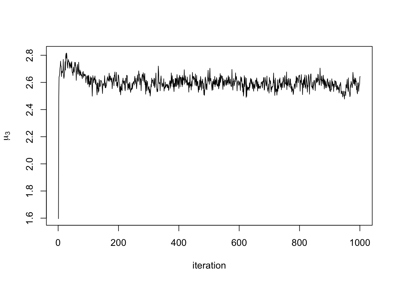
More specifically, extract_chains() returns a list with
4 elements. First, recall that M is the number of input
classes, D is the dimension of the data, and let
iterations be nstep+1. The output from
extract_chains() contains:
mu_chains: a list withMelements, each element a matrix of dimensioniterations x D.mu_chains[[i]]is the MCMC samples for the mean vector of clusteri.Sigma_chains: a list withMelements, each element an array of dimensionD x D x iterations.Sigma_chains[[i]]is the MCMC samples for the covariance matrix of clusteri.prop_chain: A matrix of dimensionM x iterations, containing the MCMC samples for the mixing proportions of each class.z_chain: A matrix of dimensionn x iterations, containing the MCMC samples for the class labels of each observation. These labels correspond to the row indices ofretained_classes(above).
These posterior samples can be used for many downstream analyses.