Computing prior probabilities
Last updated: 2019-07-17
Checks: 5 1
Knit directory: lieb/
This reproducible R Markdown analysis was created with workflowr (version 1.3.0). The Checks tab describes the reproducibility checks that were applied when the results were created. The Past versions tab lists the development history.
The R Markdown file has unstaged changes. To know which version of the R Markdown file created these results, you’ll want to first commit it to the Git repo. If you’re still working on the analysis, you can ignore this warning. When you’re finished, you can run wflow_publish to commit the R Markdown file and build the HTML.
Great job! The global environment was empty. Objects defined in the global environment can affect the analysis in your R Markdown file in unknown ways. For reproduciblity it’s best to always run the code in an empty environment.
The command set.seed(20190717) was run prior to running the code in the R Markdown file. Setting a seed ensures that any results that rely on randomness, e.g. subsampling or permutations, are reproducible.
Great job! Recording the operating system, R version, and package versions is critical for reproducibility.
Nice! There were no cached chunks for this analysis, so you can be confident that you successfully produced the results during this run.
Great! You are using Git for version control. Tracking code development and connecting the code version to the results is critical for reproducibility. The version displayed above was the version of the Git repository at the time these results were generated.
Note that you need to be careful to ensure that all relevant files for the analysis have been committed to Git prior to generating the results (you can use wflow_publish or wflow_git_commit). workflowr only checks the R Markdown file, but you know if there are other scripts or data files that it depends on. Below is the status of the Git repository when the results were generated:
Ignored files:
    Ignored:    .DS_Store
    Ignored:    .Rhistory
    Ignored:    analysis/.Rhistory
    Ignored:    analysis/pairwise_fitting_cache/
    Ignored:    docs/.DS_Store
    Ignored:    output/.DS_Store

Untracked files:
    Untracked:  docs/figure/

Unstaged changes:
    Modified:   analysis/priors.Rmd
Note that any generated files, e.g. HTML, png, CSS, etc., are not included in this status report because it is ok for generated content to have uncommitted changes.
These are the previous versions of the R Markdown and HTML files. If you’ve configured a remote Git repository (see ?wflow_git_remote), click on the hyperlinks in the table below to view them.
| File | Version | Author | Date | Message |
|---|---|---|---|---|
| Rmd | 2faf446 | hillarykoch | 2019-07-17 | update about page |
| html | 2faf446 | hillarykoch | 2019-07-17 | update about page |
| Rmd | 8278253 | hillarykoch | 2019-07-17 | update about page |
| html | 8278253 | hillarykoch | 2019-07-17 | update about page |
| html | 2177dfa | hillarykoch | 2019-07-17 | update about page |
| Rmd | 8b30694 | hillarykoch | 2019-07-17 | update about page |
| html | 8b30694 | hillarykoch | 2019-07-17 | update about page |
| html | e36b267 | hillarykoch | 2019-07-17 | update about page |
| html | a991668 | hillarykoch | 2019-07-17 | update about page |
| html | a36d893 | hillarykoch | 2019-07-17 | update about page |
| html | e8e54b7 | hillarykoch | 2019-07-17 | update about page |
| html | f47c013 | hillarykoch | 2019-07-17 | update about page |
| Rmd | 50cf23e | hillarykoch | 2019-07-17 | make skeleton |
| html | 50cf23e | hillarykoch | 2019-07-17 | make skeleton |
—Special considerations: this portion is highly parallelizable—
We are now just about ready to set up our MCMC. First, we need to determine the hyperparameters in the priors of our Gaussian mixture. These are all calculated in an empirical Bayesian manner – that is, we can recycle information from the pairwise fits to inform our priors in the full-information mixture. This task can be split into 2 sub-tasks:
computing the prior hyperparameters for the cluster mixing weights
computing every other hyperparameter
The former is the most essential, as it helps us remove more candidate latent classes, ensuring that the number of clusters is fewer than the number of observations. An important note: this is the only step of LIEB that requires some sort of human intervention, but it does need to happen. A threshold, called \(\delta\) in the manuscript, determines how strict one is about including classes in the final model. \(\delta\in\{0,1,\ldots,\hat{M}\}\), where \(\hat{M}\) is the number of candidate latent classes determined by the get_reduced_classes() function, as calculated in the previous step. We will get into selecting \(\delta\) shortly.
To get the prior weights on each candidate latent class, use the function get_prior_weights(). This function defaults to the settings used in the LIEB manuscript. The user can specify:
reduced_classes: the matrix of candidate latent classes generated byget_reduced_classes()fits: the list of pairwise fits generated byget_pairwise_fits()parallel: logical specifying if the analysis should be run in parallel (defaults to FALSE)ncores: if in parallel, how many cores to use. Defaults to 20.delta: this is the range of thresholds to try, but it will defaults to a sequence of all possible thresholds.
NB: while parallelization is always available here, it is not always necessary. Speed of this portion depends on sample size, dimension, and the number of candidate latent classes (in reduced_classes).
Now, we are ready to compute the prior weights.
# Read in the candidate latent classes produced in the last step
reduced_classes <- readr::read_tsv("output/red_class.txt", col_names = FALSE)

# load in the pairwise fits from the first step
# (in this example case, I am simply loading the data from the package)
data("fits")

# Compute the prior weights
prior_weights <- get_prior_weights(reduced_classes, fits, parallel = FALSE)
prior_weights is a list of vectors. Each vector corresponds to the computed prior weights for a given value of \(\delta\). Here, prior_weights[[m]] corresponds to the prior weights when \(\delta = m-1\). We can plot how the number of latent classes included in the final model changes as we relax \(\delta\).
# this is just grabbing the sample size and dimension
n <- length(fits[[1]]$cluster)
D <- as.numeric(strsplit(tail(names(fits),1), "_")[[1]][2])

# to avoid degenerate distributions, we will only keep clusters such that the prior
# weight times the sample size is greater than the dimension.
plot(0:nrow(reduced_classes), sapply(prior_weights, function(X) sum(X * n > D)), ylab = "number of retained classes", xlab = expression(delta))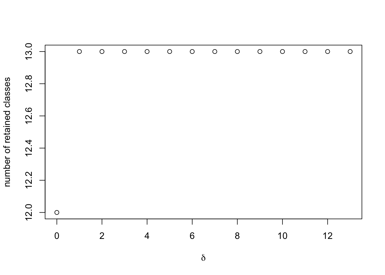
This toy example is much cleaner than a real data set, but typically we expect to see that, as we relax \(\delta\) away from 0, more classes are included in the final model. We have not identified a uniformly best way to select \(\delta\); a decent rule of thumb has simply been to include as many classes as one can while retaining computational feasibility, and selecting the smallest value of \(\delta\) that gives this result. In this toy example, we might as well retain all classes, and thus select the prior weights corresponding to \(\delta = 1\).
sessionInfo()R version 3.5.2 (2018-12-20)
Platform: x86_64-apple-darwin15.6.0 (64-bit)
Running under: macOS Sierra 10.12.6
Matrix products: default
BLAS: /Library/Frameworks/R.framework/Versions/3.5/Resources/lib/libRblas.0.dylib
LAPACK: /Library/Frameworks/R.framework/Versions/3.5/Resources/lib/libRlapack.dylib
locale:
[1] en_US.UTF-8/en_US.UTF-8/en_US.UTF-8/C/en_US.UTF-8/en_US.UTF-8
attached base packages:
[1] stats graphics grDevices utils datasets methods base
other attached packages:
[1] LIEB_0.1.0
loaded via a namespace (and not attached):
[1] Rcpp_1.0.1 compiler_3.5.2 pillar_1.3.1
[4] git2r_0.24.0 plyr_1.8.4 workflowr_1.3.0
[7] iterators_1.0.10 tools_3.5.2 testthat_2.0.1
[10] digest_0.6.18 lattice_0.20-38 evaluate_0.13
[13] tibble_2.0.1 pkgconfig_2.0.2 rlang_0.3.1
[16] igraph_1.2.4 foreach_1.4.4 rstudioapi_0.9.0
[19] yaml_2.2.0 parallel_3.5.2 mvtnorm_1.0-11
[22] LaplacesDemon_16.1.1 xfun_0.5 coda_0.19-2
[25] dplyr_0.8.0.1 stringr_1.4.0 knitr_1.22
[28] fs_1.2.6 hms_0.4.2 grid_3.5.2
[31] rprojroot_1.3-2 tidyselect_0.2.5 glue_1.3.0
[34] R6_2.4.0 JuliaCall_0.16.4 rmarkdown_1.12
[37] purrr_0.3.1 readr_1.3.1 magrittr_1.5
[40] whisker_0.3-2 backports_1.1.3 codetools_0.2-16
[43] htmltools_0.3.6 abind_1.4-5 assertthat_0.2.1
[46] nimble_0.7.0.1 stringi_1.3.1 doParallel_1.0.14
[49] crayon_1.3.4