Accounting for technical batch effects: Response to infection with Mycobacterium tuberculosis
John Blischak
2018-08-09
Last updated: 2019-02-26
Checks: 6 0
Knit directory: dc-bioc-limma/analysis/
This reproducible R Markdown analysis was created with workflowr (version 1.2.0.9000). The Report tab describes the reproducibility checks that were applied when the results were created. The Past versions tab lists the development history.
Great! Since the R Markdown file has been committed to the Git repository, you know the exact version of the code that produced these results.
Great job! The global environment was empty. Objects defined in the global environment can affect the analysis in your R Markdown file in unknown ways. For reproduciblity it’s best to always run the code in an empty environment.
The command set.seed(12345) was run prior to running the code in the R Markdown file. Setting a seed ensures that any results that rely on randomness, e.g. subsampling or permutations, are reproducible.
Great job! Recording the operating system, R version, and package versions is critical for reproducibility.
Nice! There were no cached chunks for this analysis, so you can be confident that you successfully produced the results during this run.
Great! You are using Git for version control. Tracking code development and connecting the code version to the results is critical for reproducibility. The version displayed above was the version of the Git repository at the time these results were generated.
Note that you need to be careful to ensure that all relevant files for the analysis have been committed to Git prior to generating the results (you can use wflow_publish or wflow_git_commit). workflowr only checks the R Markdown file, but you know if there are other scripts or data files that it depends on. Below is the status of the Git repository when the results were generated:
Ignored files:
    Ignored:    .Rhistory
    Ignored:    .Rproj.user/

Untracked files:
    Untracked:  analysis/table-s1.txt
    Untracked:  analysis/table-s2.txt
    Untracked:  code/tb-scratch.R
    Untracked:  data/counts_per_sample.txt
    Untracked:  docs/style.css
    Untracked:  docs/table-s1.txt
    Untracked:  docs/table-s2.txt
    Untracked:  factorial-dox.rds
Note that any generated files, e.g. HTML, png, CSS, etc., are not included in this status report because it is ok for generated content to have uncommitted changes.
These are the previous versions of the R Markdown and HTML files. If you’ve configured a remote Git repository (see ?wflow_git_remote), click on the hyperlinks in the table below to view them.
| File | Version | Author | Date | Message |
|---|---|---|---|---|
| html | 2372aa1 | John Blischak | 2019-01-09 | Build site. |
| html | f440a87 | John Blischak | 2018-08-20 | Build site. |
| html | f2c0198 | John Blischak | 2018-08-09 | Build site. |
| Rmd | 6893542 | John Blischak | 2018-08-09 | Organize analysis of batch effects in TB data. |
An example of diagnosing and correcting batch effects from one of my own studies on the response to infection with Mycobacterium tuberculosis (paper, code, data).
Setup
library(dplyr)
library(limma)
library(edgeR)
# Have to load Biobase after dplyr so that exprs function works
library(Biobase)
Download data.
file_url <- "https://bitbucket.org/jdblischak/tb-data/raw/bc0f64292eb8c42a372b3a2d50e3d871c70c202e/counts_per_sample.txt"
full <- read.delim(file_url, stringsAsFactors = FALSE)
Convert to ExpressionSet.
dim(full)[1] 156 19419full <- full[order(full$dir), ]
rownames(full) <- paste(full$ind, full$bact, full$time, sep = ".")
x <- t(full[, grep("ENSG", colnames(full))])
p <- full %>% select(ind, bact, time, extr, rin)
stopifnot(colnames(x) == rownames(p))
eset <- ExpressionSet(assayData = x,
phenoData = AnnotatedDataFrame(p))Filter lowly expressed genes.
keep <- rowSums(cpm(exprs(eset)) > 1) > 6
sum(keep)
[1] 12728eset <- eset[keep, ]
dim(eset)Features Samples
12728 156 Normalize with TMM.
norm_factors <- calcNormFactors(exprs(eset))
exprs(eset) <- cpm(exprs(eset), lib.size = colSums(exprs(eset)) * norm_factors,
                   log = TRUE)
plotDensities(eset, legend = FALSE)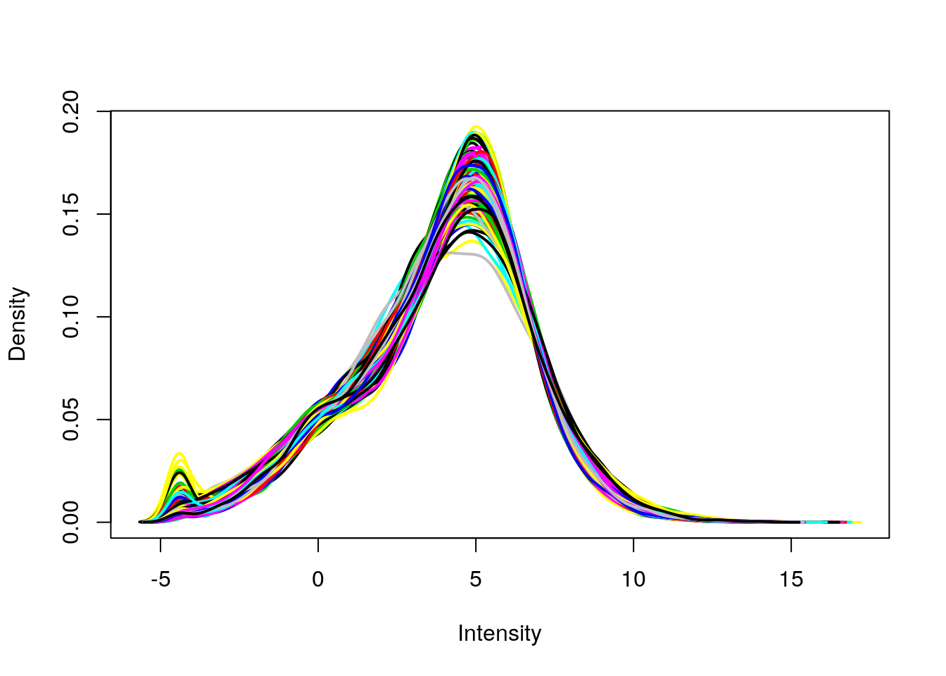
Clean up phenotype data frame to focus on early versus late timepoint for this example.
pData(eset)[, "infection"] <- ifelse(pData(eset)[, "bact"] == "none",
                                     "con", "inf")

pData(eset)[, "time"] <- ifelse(pData(eset)[, "time"] == 4,
                                "early", "late")

pData(eset)[, "batch"] <- sprintf("b%02d", pData(eset)[, "extr"])

table(pData(eset)[, c("time", "batch")])
batch
time b01 b02 b03 b04 b05 b06 b07 b08 b09 b10 b11 b12 b13
early 4 4 4 4 4 4 4 4 4 4 4 4 6
late 8 8 8 8 8 8 8 8 8 8 8 8 6Remove batch effect
Visualize principal components 1 and 2 for the original data.
plotMDS(eset, labels = pData(eset)[, "time"], gene.selection = "common")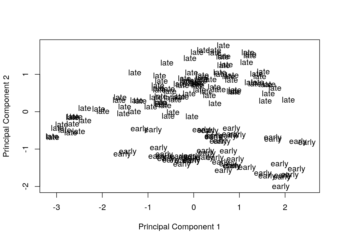
Remove the effect of the technical variables: batch (discrete) and RIN (continuous; a measure of RNA quality).
exprs(eset) <- removeBatchEffect(eset, batch = pData(eset)[, "batch"],
                                 covariates = pData(eset)[, "rin"])
Visualize principal components 1 and 2 for the corrected data.
plotMDS(eset, labels = pData(eset)[, "time"], gene.selection = "common")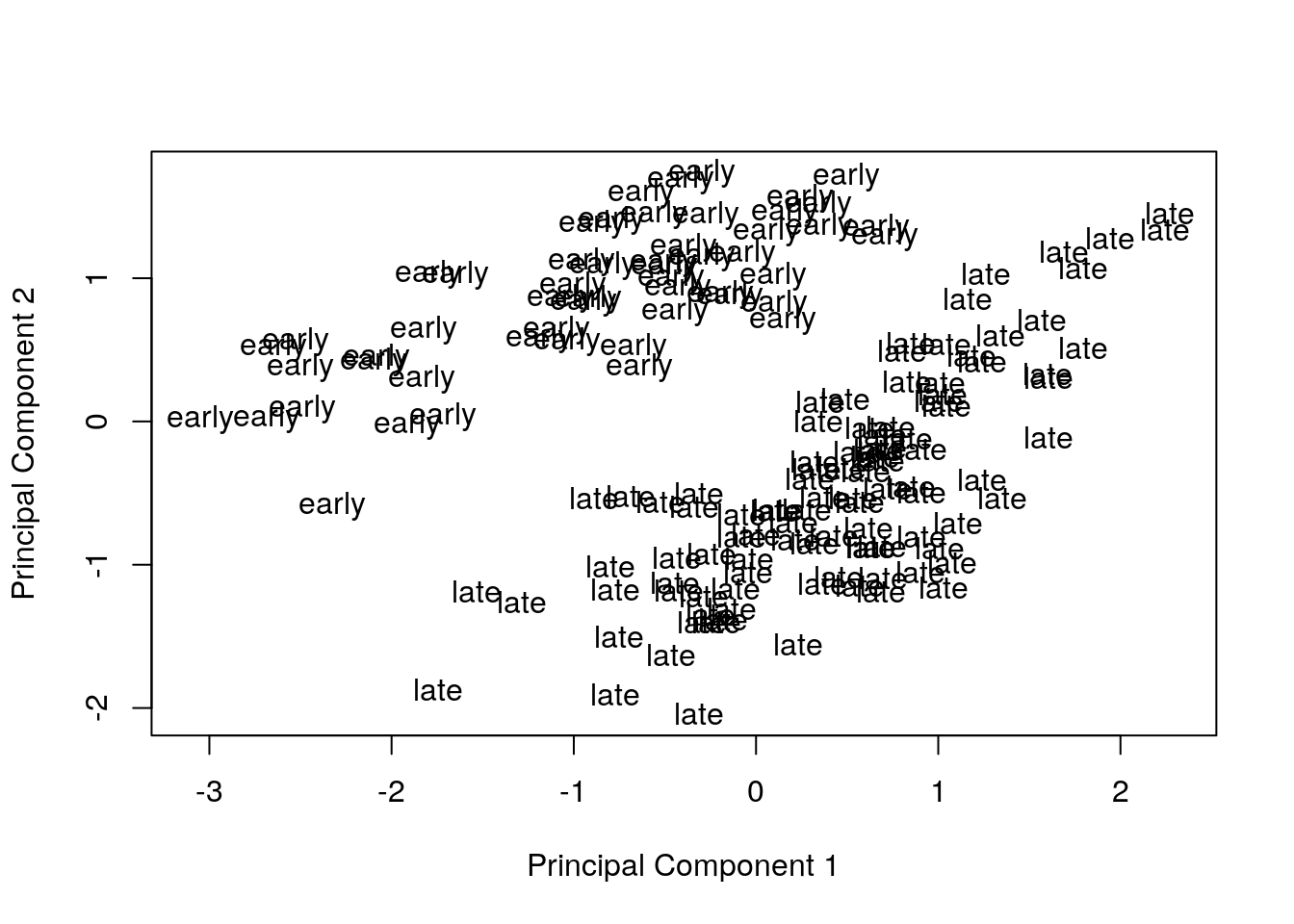
sessionInfo()R version 3.5.2 (2018-12-20)
Platform: x86_64-pc-linux-gnu (64-bit)
Running under: Ubuntu 18.04.2 LTS
Matrix products: default
BLAS: /usr/lib/x86_64-linux-gnu/atlas/libblas.so.3.10.3
LAPACK: /usr/lib/x86_64-linux-gnu/atlas/liblapack.so.3.10.3
locale:
[1] LC_CTYPE=en_US.UTF-8 LC_NUMERIC=C
[3] LC_TIME=en_US.UTF-8 LC_COLLATE=en_US.UTF-8
[5] LC_MONETARY=en_US.UTF-8 LC_MESSAGES=en_US.UTF-8
[7] LC_PAPER=en_US.UTF-8 LC_NAME=C
[9] LC_ADDRESS=C LC_TELEPHONE=C
[11] LC_MEASUREMENT=en_US.UTF-8 LC_IDENTIFICATION=C
attached base packages:
[1] parallel stats graphics grDevices utils datasets methods
[8] base
other attached packages:
[1] Biobase_2.42.0 BiocGenerics_0.28.0 edgeR_3.24.3
[4] limma_3.38.3 dplyr_0.8.0.1
loaded via a namespace (and not attached):
[1] Rcpp_1.0.0 knitr_1.21 whisker_0.3-2
[4] magrittr_1.5 workflowr_1.2.0.9000 tidyselect_0.2.5
[7] lattice_0.20-38 R6_2.4.0 rlang_0.3.1
[10] stringr_1.4.0 tools_3.5.2 grid_3.5.2
[13] xfun_0.5 git2r_0.24.0 htmltools_0.3.6
[16] yaml_2.2.0 rprojroot_1.2 digest_0.6.18
[19] assertthat_0.2.0 tibble_2.0.1 crayon_1.3.4
[22] purrr_0.3.0 fs_1.2.6 glue_1.3.0
[25] evaluate_0.13 rmarkdown_1.11 stringi_1.3.1
[28] compiler_3.5.2 pillar_1.3.1 backports_1.1.3
[31] locfit_1.5-9.1 pkgconfig_2.0.2