MLD_pCO2
Jens Daniel Müller & Lara Burchardt
16 March, 2020
Last updated: 2020-03-16
Checks: 7 0
Knit directory: Baltic_Productivity/
This reproducible R Markdown analysis was created with workflowr (version 1.6.0). The Checks tab describes the reproducibility checks that were applied when the results were created. The Past versions tab lists the development history.
Great! Since the R Markdown file has been committed to the Git repository, you know the exact version of the code that produced these results.
Great job! The global environment was empty. Objects defined in the global environment can affect the analysis in your R Markdown file in unknown ways. For reproduciblity it’s best to always run the code in an empty environment.
The command set.seed(20191017) was run prior to running the code in the R Markdown file. Setting a seed ensures that any results that rely on randomness, e.g. subsampling or permutations, are reproducible.
Great job! Recording the operating system, R version, and package versions is critical for reproducibility.
Nice! There were no cached chunks for this analysis, so you can be confident that you successfully produced the results during this run.
Great job! Using relative paths to the files within your workflowr project makes it easier to run your code on other machines.
Great! You are using Git for version control. Tracking code development and connecting the code version to the results is critical for reproducibility. The version displayed above was the version of the Git repository at the time these results were generated.
Note that you need to be careful to ensure that all relevant files for the analysis have been committed to Git prior to generating the results (you can use wflow_publish or wflow_git_commit). workflowr only checks the R Markdown file, but you know if there are other scripts or data files that it depends on. Below is the status of the Git repository when the results were generated:
Ignored files:
    Ignored:    .Rhistory
    Ignored:    .Rproj.user/
    Ignored:    data/ARGO/
    Ignored:    data/Finnmaid/
    Ignored:    data/GETM/
    Ignored:    data/OSTIA/
    Ignored:    data/_merged_data_files/
    Ignored:    data/_merged_data_files_2019V1/
    Ignored:    data/_summarized_data_files/
    Ignored:    data/_summarized_data_files_2019V1/

Unstaged changes:
    Deleted:    code/SSS.Rmd
Note that any generated files, e.g. HTML, png, CSS, etc., are not included in this status report because it is ok for generated content to have uncommitted changes.
There are no past versions. Publish this analysis with wflow_publish() to start tracking its development.
1 Regional pCO2 and mixed layer depths
Within this chapter we relate Finnmaid pCO2 observations and different mixed layer depths estimates from GETM within the Northern Gotland Sea area.
1.1 GETM mixed layer depths
As a first step we read-in following mixed layer depths estimated from GETM:
- MLD Age 1: Penetration depth of a surface tracer injected into the surface after 1 days
- MLD Age 3: Penetration depth of a surface tracer injected into the surface after 3 days
- MLD Age 5: Penetration depth of a surface tracer injected into the surface after 5 days
- MLD Rho: Mixed layer depth based on a density criterion
- MLD Tke: Mixing layer depth based on the turbulent kinetic energy and the density stratification
var_all <- c("mld_age_1", "mld_age_3", "mld_age_5", "mld_rho", "mld_tke")

filesList_2d <- list.files(path= "data", pattern = "Finnmaid.E.2d.20", recursive = TRUE)

file <- filesList_2d[8]
nc <- nc_open(paste("data/", file, sep = ""))

lon <- ncvar_get(nc, "lonc")
lat <- ncvar_get(nc, "latc", verbose = F)
corvector <- c(1:544)
nc_close(nc)

cor_space <- as.data.frame(cbind(lon, lat, corvector))


rm(file, nc)

for (a in 1:5){

  var <- var_all[a]


for (n in 1:length(filesList_2d)) {

#file <- filesList_2d[8]
file <- filesList_2d[n]

nc <- nc_open(paste("data/", file, sep = ""))

time_units <- nc$dim$time$units %>%     #we read the time unit from the netcdf file to calibrate the time
    substr(start = 15, stop = 33) %>%   #calculation, we take the relevant information from the string
    ymd_hms()                           # and transform it to the right format

t <- time_units + ncvar_get(nc, "time")

array <- ncvar_get(nc, var) # store the data in a 2-dimensional array
dim(array) # should be 2d with dimensions: 544 coordinate, 31d*(24h/d/3h)=248 time steps

array <- as.data.frame(t(array), xy=TRUE)
array <- as_tibble(array)

#use corvector (1:544)
gt_mld_hov_part <- array %>%
  set_names(as.character(corvector)) %>%
  mutate(date_time = t) %>%
  gather("corvector", "value", 1:length(corvector)) %>%
  mutate(corvector = as.numeric(corvector),
  date = as.Date(date_time)) %>%
  select(-date_time) %>%
  group_by(date, corvector) %>%
  summarise_all("mean") %>%
  ungroup() %>%
  rename(mld = value)


if (exists("gt_mld_hov")) {gt_mld_hov <- bind_rows(gt_mld_hov, gt_mld_hov_part)
  }else {gt_mld_hov <- gt_mld_hov_part}

  nc_close(nc)
  rm(array, nc, t, gt_mld_hov_part)
  print(n) # to see working progress
}

print(paste("gt_", var, "_hov.csv", sep = "")) # to see working progress

gt_mld_hov %>%
  vroom_write(here::here("data/_summarized_data_files/", file = paste("gt_", var, "_hov.csv", sep = "")))

rm(gt_mld_hov, n, file, time_units, var)
}

rm(a, filesList_2d, var_all, lat, lon)
1.2 Finnmaid pCO2
In the following we extract Finnmaid pCO2 data for the Northern Gotland Sea. For each crossing of the ferry, mean, minimum, maximum and the standard deviation of pCO2 are calculated.
nc <- nc_open(paste("data/Finnmaid/", "FM_all_2019_on_standard_tracks.nc", sep = ""))

var <- "pCO2_east"

# read required vectors from netcdf file
route <- ncvar_get(nc, "route")
route <- unlist(strsplit(route, ""))
date_time <- ncvar_get(nc, "time")
latitude_east <- ncvar_get(nc, "latitude_east")

array <- ncvar_get(nc, var) # store the data in a 2-dimensional array
#dim(array) # should have 2 dimensions: 544 coordinate, 2089 time steps

  fillvalue <- ncatt_get(nc, var, "_FillValue")
  array[array == fillvalue$value] <- NA
  rm(fillvalue)

  for (i in seq(1,length(route),1)){


    if(route[i] == select_route) {
      slice <- array[i,]

      value <- mean(slice[latitude_east > low_lat & latitude_east < high_lat], na.rm = TRUE)
      sd    <- sd(slice[latitude_east > low_lat & latitude_east < high_lat], na.rm = TRUE)
      min   <- min(slice[latitude_east > low_lat & latitude_east < high_lat], na.rm = TRUE)
      max   <- max(slice[latitude_east > low_lat & latitude_east < high_lat], na.rm = TRUE)
      date <- ymd("2000-01-01") + date_time[i]

      temp <- bind_cols(date = date, var=var, value = value, sd = sd, min = min, max = max)

      if (exists("fm_pco2_ngs", inherits = FALSE)){
        fm_pco2_ngs <- bind_rows(fm_pco2_ngs, temp)
      } else{fm_pco2_ngs <- temp}

      rm(temp, value, date, sd, min, max)

    }
  }
nc_close(nc)

fm_pco2_ngs$date_time <- as.POSIXct(fm_pco2_ngs$date) %>%
  cut.POSIXt(breaks = "days") %>%
  round.POSIXt(units = "days") %>%
  as.POSIXct(tz = "UTC")
fm_pco2_ngs <- fm_pco2_ngs %>%
  select(-c(date))

fm_pco2_ngs %>%
  vroom_write(here::here("data/_summarized_data_files/", file = "fm_pco2_ngs.csv"))

rm(array, nc, slice, var, fm_pco2_ngs, latitude_east, date_time, route,i)
1.3 Data merging
We want a datafile including the pCO2 values, as measured from the Finnmaid, as well as all five mixed layer depth parameters.
ts_pco2_ngs <- vroom::vroom(here::here("data/_summarized_data_files/", file = "fm_pco2_ngs.csv"))#, na = c("NA", "NaN", "Inf", "-Inf"))
ts_mld_age_1_hov <- vroom::vroom(here::here("data/_summarized_data_files/", file = "gt_mld_age_1_hov.csv"))
ts_mld_age_3_hov <- vroom::vroom(here::here("data/_summarized_data_files/", file = "gt_mld_age_3_hov.csv"))
ts_mld_age_5_hov <- vroom::vroom(here::here("data/_summarized_data_files/", file = "gt_mld_age_5_hov.csv"))
ts_mld_rho_hov <- vroom::vroom(here::here("data/_summarized_data_files/", file = "gt_mld_rho_hov.csv"))
ts_mld_tke_hov <- vroom::vroom(here::here("data/_summarized_data_files/", file = "gt_mld_tke_hov.csv"))

#pCO2 Finnmaid
ts_pco2_ngs <- ts_pco2_ngs %>%
  transmute( value_pCO2 = value, sd_pCO2 = sd, min_pCO2 = min, max_pCO2 = max, date = date_time)


filesList_2d <- list.files(path= "data", pattern = "Finnmaid.E.2d.20", recursive = TRUE)

file <- filesList_2d[8]
nc <- nc_open(paste("data/", file, sep = ""))
lon <- ncvar_get(nc, "lonc")
lat <- ncvar_get(nc, "latc", verbose = F)
corvector <- c(1:544)
nc_close(nc)
cor_space <- as.data.frame(cbind(lon, lat, corvector))

cor_space_restriction <- cor_space %>%
  filter(lat > low_lat, lat<high_lat)
low_cor <- min(cor_space_restriction$corvector)
high_cor <- max(cor_space_restriction$corvector)

#mld_age_1
ts_mld_age_1_ngs <- ts_mld_age_1_hov %>%
  filter(corvector > low_cor, corvector<high_cor) %>%
  group_by(date) %>%
  summarise_all(list(value=~mean(.,na.rm=TRUE))) %>%
  ungroup() %>%
  transmute( date = date, corvector = corvector_value, value_mld1 = mld_value)
#mld_age_3
ts_mld_age_3_ngs <- ts_mld_age_3_hov %>%
  filter(corvector > low_cor, corvector<high_cor) %>%
  group_by(date) %>%
  summarise_all(list(value=~mean(.,na.rm=TRUE))) %>%
  ungroup() %>%
  transmute( date = date, corvector = corvector_value, value_mld3 = mld_value)
#mld_age_5
ts_mld_age_5_ngs <- ts_mld_age_5_hov %>%
  filter(corvector > low_cor, corvector<high_cor) %>%
  group_by(date) %>%
  summarise_all(list(value=~mean(.,na.rm=TRUE))) %>%
  ungroup() %>%
  transmute( date = date, corvector = corvector_value, value_mld5 = mld_value)
#mld_rho
ts_mld_rho_ngs <- ts_mld_rho_hov %>%
  filter(corvector > low_cor, corvector<high_cor) %>%
  group_by(date) %>%
  summarise_all(list(value=~mean(.,na.rm=TRUE))) %>%
  ungroup() %>%
  transmute( date = date, corvector = corvector_value, value_mldrho = mld_value)
#mld_tke
ts_mld_tke_ngs <- ts_mld_tke_hov %>%
  filter(corvector > low_cor, corvector<high_cor) %>%
  group_by(date) %>%
  summarise_all(list(value=~mean(.,na.rm=TRUE))) %>%
  ungroup() %>%
  transmute( date = date, corvector = corvector_value, value_mldtke = mld_value)


ts_mld_ngs <- bind_cols(ts_mld_age_1_ngs, ts_mld_age_3_ngs, ts_mld_age_5_ngs, ts_mld_rho_ngs, ts_mld_tke_ngs)
ts_mld_ngs <- ts_mld_ngs %>%
  select(date, corvector, value_mld1, value_mld3, value_mld5, value_mldrho, value_mldtke) %>%
  mutate(date = as.POSIXct(date))

ts_mld_ngs$date <- ts_mld_ngs$date %>%
  cut.POSIXt(breaks = "days") %>%
  round.POSIXt(units = "days") %>%
  as.POSIXct(tz = "UTC")

ts_mld_pco2_ngs <- full_join(ts_pco2_ngs, ts_mld_ngs, by = "date")

ts_mld_pco2_ngs %>%
  vroom_write(here::here("data/_merged_data_files/", file = "gt_mld_fm_pco2_ngs.csv"))
1.4 Timeseries plots
ts_mld_pco2_ngs <- vroom::vroom(here::here("data/_merged_data_files/", file = "gt_mld_fm_pco2_ngs.csv"))

ts_xts <- xts(cbind(ts_mld_pco2_ngs$value_mld1,ts_mld_pco2_ngs$value_mld3, ts_mld_pco2_ngs$value_mld5, ts_mld_pco2_ngs$value_mldrho, ts_mld_pco2_ngs$value_mldtke), order.by = ts_mld_pco2_ngs$date)
names(ts_xts) <- c("MLD Age 1", "MLD Age 3", "MLD Age 5", "MLD Rho", "MLD Tke")
ts_pco2_xts <- xts(cbind(ts_mld_pco2_ngs$value_pCO2, ts_mld_pco2_ngs$min_pCO2, ts_mld_pco2_ngs$max_pCO2), order.by = ts_mld_pco2_ngs$date)
names(ts_pco2_xts) <- c("pCO2 Finnmaid", "lwr", "upr")

ts_xts %>%
  dygraph(group = "MLD") %>%
  dyRangeSelector(dateWindow = c("2014-01-01", "2016-12-31")) %>%
  dySeries("MLD Age 1") %>%
  dySeries("MLD Age 3", color = "red") %>%
  dyAxis("y", label = "MLD [m]") %>%
  dyOptions(drawPoints = TRUE, pointSize = 1.5, connectSeparatedPoints=TRUE, strokeWidth=0.5)
ts_pco2_xts %>%
dygraph(group = "MLD") %>%
dyRangeSelector(dateWindow = c("2014-01-01", "2016-12-31")) %>%
dySeries(c("lwr", "pCO2 Finnmaid","upr")) %>%
dyAxis("y", label = "") %>%
dyOptions(drawPoints = TRUE, pointSize = 1.5, connectSeparatedPoints=TRUE, strokeWidth=0.5,
drawAxesAtZero=TRUE)rm(ts_mld_pco2_ngs, ts_xts, ts_pco2_xts)2 Basin-wide pCO2 and mixed layer depth
2.1 GETM mixed layer depths
The dataset for the regional analysis of mixed layer depths and pCO2 were written such, that already the complete information was calculated for the GETM data.
2.2 Finnmaid pCO2
The pCO2 measurments are also to be analysed for the whole basin next. Same as for the SST analysis, the route is divided in 2 km grids (startpoint Travemuende). That results in 544 coordinate points in every transect. The corresponding coordinate number (1:544) is added to the dataset, with the exact longitude and lattitude coordinates.
#Prepare data for Hovmoeller Plot

nc <- nc_open(paste("data/Finnmaid/", "FM_all_2019_on_standard_tracks.nc", sep = ""))

var <- "pCO2_east"

# read required vectors from netcdf file
route <- ncvar_get(nc, "route")
route <- unlist(strsplit(route, ""))
date_time <- ncvar_get(nc, "time")
latitude_east <- ncvar_get(nc, "latitude_east")
longitude_east <-ncvar_get(nc, "longitude_east")
date_time_o <- ncvar_get(nc, "otime_east")

  array <- ncvar_get(nc, var) # store the data in a 2-dimensional array
  #dim(array) # should have 2 dimensions: 544 coordinate, 2089 time steps

  fillvalue <- ncatt_get(nc, var, "_FillValue")
  array[array == fillvalue$value] <- NA
  rm(fillvalue)

  cor_vector <- c(1:544)

  #i <- 5

  for (i in seq(1,length(route),1)){


    if(route[i] == select_route) {
      slice <- array[i,]          #define slice of the data, per row (per measurment day)
      value <- slice
      date <- ymd("2000-01-01") + date_time[i]

      #if detailed date/time information is needed: uncomment that
      #date <- as.Date(c(1:544))   # set up "date" variable to be overwritten later, needs to be "Date" object
      #for (a in seq(1,length(latitude_east),1)){              # for slice i the corresponding 544 transect steps are
      #temp_time <- ymd("2000-01-01") + date_time_o[i,a]       # adjoined by corresponding time ("otime_east")
      #date[a] <- temp_time
      #}
      #temp <- bind_cols(value = value, lon = longitude_east, lat = latitude_east,
      #corvector =   cor_vector, date_time = date)
      #temp$date_time <- as.POSIXct(temp$date_time)

      #when detailed time/date information is needed, comment the following
      temp <- bind_cols(value = value, lon = longitude_east, lat = latitude_east,
      corvector =  cor_vector)
      temp$date <- date
      #

      if (exists("fm_pco2_hov", inherits = FALSE)){
        fm_pco2_hov <- bind_rows(fm_pco2_hov, temp)
      } else{fm_pco2_hov <- temp}

      rm(temp, value, date)
    }
    print(i)
  }
nc_close(nc)

fm_pco2_hov <- fm_pco2_hov %>%
  mutate(value_pCO2_Finn = value) %>%
  select(-c(value))

fm_pco2_hov %>%
  vroom_write(here::here("data/_summarized_data_files/", file = "fm_pco2_hov.csv"))

rm(array, nc, slice, var, date_time_o, cor_vector, date_time, latitude_east,longitude_east,route,i)
2.3 Data Merging without lat restrictions
ts_pCO2_hov <- vroom::vroom(here::here("data/_summarized_data_files/", file = "fm_pco2_hov.csv"))
#ts_mld_age_1_hov <- vroom::vroom(here::here("data/_summarized_data_files/", file = "gt_mld_age_1_hov.csv"))
#ts_mld_age_3_hov <- vroom::vroom(here::here("data/_summarized_data_files/", file = "gt_mld_age_3_hov.csv"))
#ts_mld_age_5_hov <- vroom::vroom(here::here("data/_summarized_data_files/", file = "gt_mld_age_5_hov.csv"))
#ts_mld_rho_hov <- vroom::vroom(here::here("data/_summarized_data_files/", file = "gt_mld_rho_hov.csv"))
#ts_mld_tke_hov <- vroom::vroom(here::here("data/_summarized_data_files/", file = "gt_mld_tke_hov.csv"))


ts_mld_age_1_hov <- ts_mld_age_1_hov %>%
    transmute( date = date, corvector = corvector, value_mld1 = mld)

ts_mld_age_3_hov <- ts_mld_age_3_hov %>%
    transmute( date = date, corvector = corvector, value_mld3 = mld)

ts_mld_age_5_hov <- ts_mld_age_5_hov %>%
    transmute( date = date, corvector = corvector, value_mld5 = mld)

ts_mld_rho_hov <- ts_mld_rho_hov %>%
    transmute( date = date, corvector = corvector, value_mldrho = mld)

ts_mld_tke_hov <- ts_mld_tke_hov %>%
    transmute( date = date, corvector = corvector, value_mldtke = mld)

ts_mld_hov <- bind_cols(ts_mld_age_1_hov, ts_mld_age_3_hov, ts_mld_age_5_hov, ts_mld_rho_hov, ts_mld_tke_hov)
ts_mld_hov <- ts_mld_hov %>%
  select(date, corvector, value_mld1, value_mld3, value_mld5, value_mldrho, value_mldtke) %>%
  mutate(date = as.POSIXct(date))

ts_mld_hov$date <- ts_mld_hov$date %>%
  cut.POSIXt(breaks = "days") %>%
  round.POSIXt(units = "days") %>%
  as.POSIXct(tz = "UTC")

ts_pCO2_hov$date <- ts_pCO2_hov$date %>%
  as.POSIXct() %>%
  cut.POSIXt(breaks = "days") %>%
  round.POSIXt(units = "days") %>%
  as.POSIXct(tz = "UTC")

ts_mld_pco2_hov <- full_join(ts_pCO2_hov, ts_mld_hov, by =c("date","corvector"))

ts_mld_pco2_hov %>%
vroom_write(here::here("data/_merged_data_files/", file = "ts_mld_pco2_hov.csv"))
2.4 Hovmoeller Plots
2.4.1 Daily GETM mld
We present Hovmoeller Plots for the 5 mixed layer depth parameters (see 5.1). The daily GETM mld values are presented as a function of time and the ships distance to Travemuende along route E. Plots are shown seperatly for each parameter and years. This timeseries represents mixed layer depth values for the parameter mld_age_1 from 2007 to 2019.
ts_mld_pco2_hov <-
  vroom::vroom(here::here("data/_merged_data_files/", file = "ts_mld_pco2_hov.csv"), guess_max = 105537)
# why guess_max so high? because the first 105536 rows of mld values are empty and when opening are interpreted as factors, which results in a parsing error

ts_mld_pco2_hov <- ts_mld_pco2_hov %>%
  mutate(date = ymd(date),
         year = year(date),
         dist.trav = corvector*2)
#mld age 1
ts_mld_pco2_hov %>%
  filter(year > 2006, year < 2019) %>%
  ggplot()+
    geom_raster(aes(date, dist.trav, fill=value_mld1))+
      scale_fill_viridis_c(name="GETM MLD Age 1 [m]",
                           limits = c(0,80),
                           direction = -1)+
      scale_x_date(expand = c(0,0))+
      scale_y_continuous(expand = c(0,0))+
      labs(y="Distance to Travemuende [km]")+
      theme_bw()+
      theme(
        axis.title.x = element_blank(),
        legend.position = "bottom",
        legend.key.width = unit(1.3, "cm"),
        legend.key.height = unit(0.3, "cm")
      )+
      facet_wrap(~year, ncol = 1, scales = "free_x")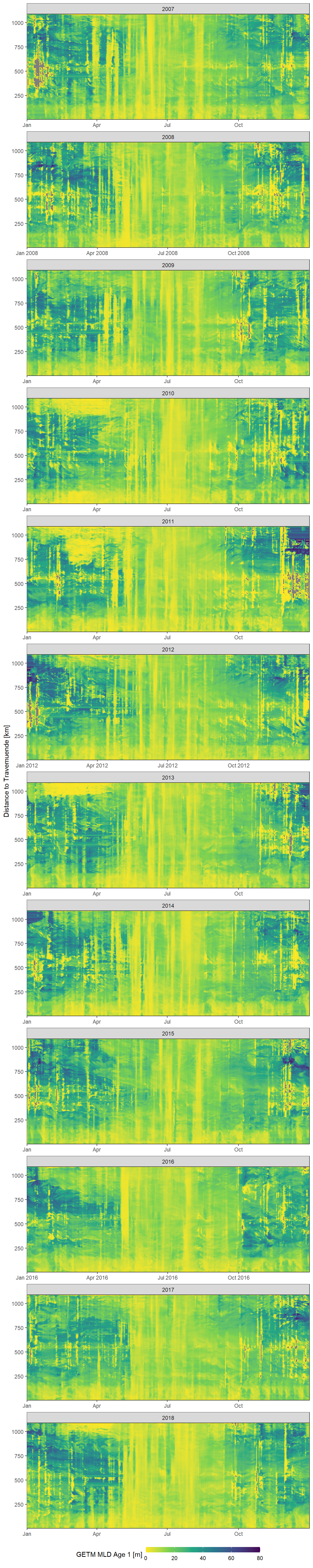
Daily mean GETM mld age 1 values as a function of time and the ships distance to Travemuende along route E.
This timeseries represents mixed layer depth values for the parameter mld_age_3 from 2007 to 2019.
#mld age 3
ts_mld_pco2_hov %>%
  filter(year > 2006, year < 2019) %>%
  ggplot()+
    geom_raster(aes(date, dist.trav, fill=value_mld3))+
      scale_fill_viridis_c(name="GETM MLD Age 3 [m]",
                           limits = c(0,80),
                           direction = -1)+
      scale_x_date(expand = c(0,0))+
      scale_y_continuous(expand = c(0,0))+
      labs(y="Distance to Travemuende [km]")+
      theme_bw()+
      theme(
        axis.title.x = element_blank(),
        legend.position = "bottom",
        legend.key.width = unit(1.3, "cm"),
        legend.key.height = unit(0.3, "cm")
      )+
      facet_wrap(~year, ncol = 1, scales = "free_x")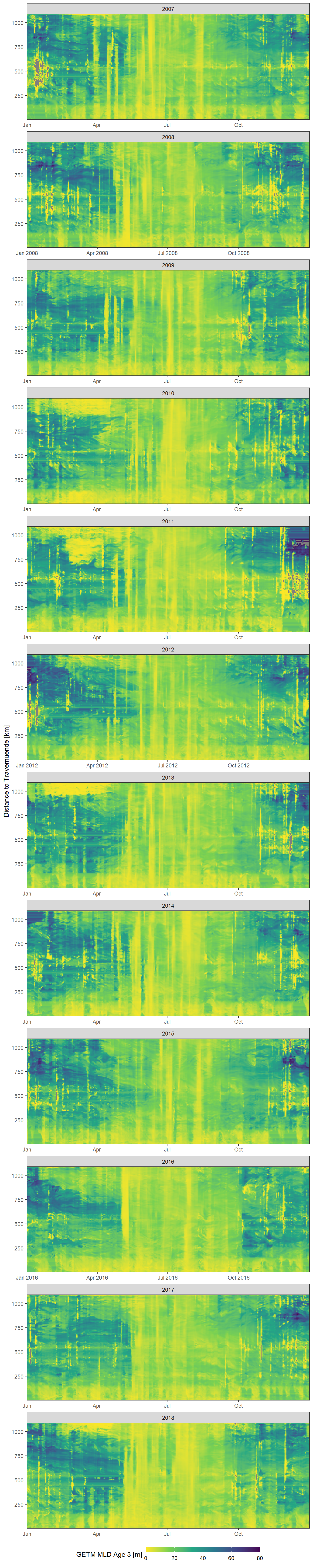
Daily mean GETM mld age 3 values as a function of time and the ships distance to Travemuende along route E.
This timeseries represents mixed layer depth values for the parameter mld_age_5 from 2007 to 2019.
#mld age 5
ts_mld_pco2_hov %>%
  filter(year > 2006, year < 2019) %>%
  ggplot()+
    geom_raster(aes(date, dist.trav, fill=value_mld5))+
      scale_fill_viridis_c(name="GETM MLD Age 5 [m]",
                           limits = c(0,80),
                           direction = -1)+
      scale_x_date(expand = c(0,0))+
      scale_y_continuous(expand = c(0,0))+
      labs(y="Distance to Travemuende [km]")+
      theme_bw()+
      theme(
        axis.title.x = element_blank(),
        legend.position = "bottom",
        legend.key.width = unit(1.3, "cm"),
        legend.key.height = unit(0.3, "cm")
      )+
      facet_wrap(~year, ncol = 1, scales = "free_x")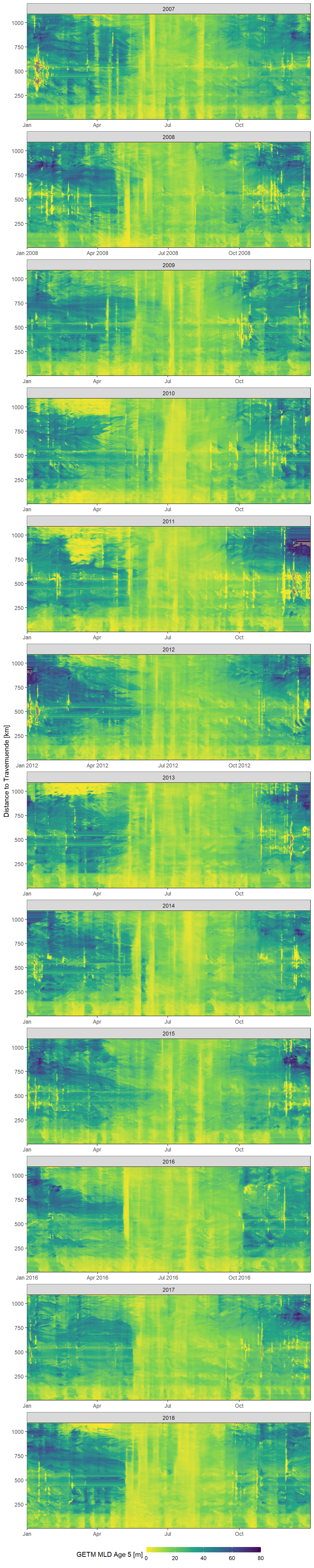
Daily mean GETM mld age 5 values as a function of time and the ships distance to Travemuende along route E.
This timeseries represents mixed layer depth values for the parameter mld_rho from 2007 to 2019.
#mld rho
ts_mld_pco2_hov %>%
  filter(year > 2006, year < 2019) %>%
  ggplot()+
    geom_raster(aes(date, dist.trav, fill=value_mldrho))+
      scale_fill_viridis_c(name="GETM MLD Rho [m]",
                           limits = c(0,80),
                           direction = -1)+
      scale_x_date(expand = c(0,0))+
      scale_y_continuous(expand = c(0,0))+
      labs(y="Distance to Travemuende [km]")+
      theme_bw()+
      theme(
        axis.title.x = element_blank(),
        legend.position = "bottom",
        legend.key.width = unit(1.3, "cm"),
        legend.key.height = unit(0.3, "cm")
      )+
      facet_wrap(~year, ncol = 1, scales = "free_x")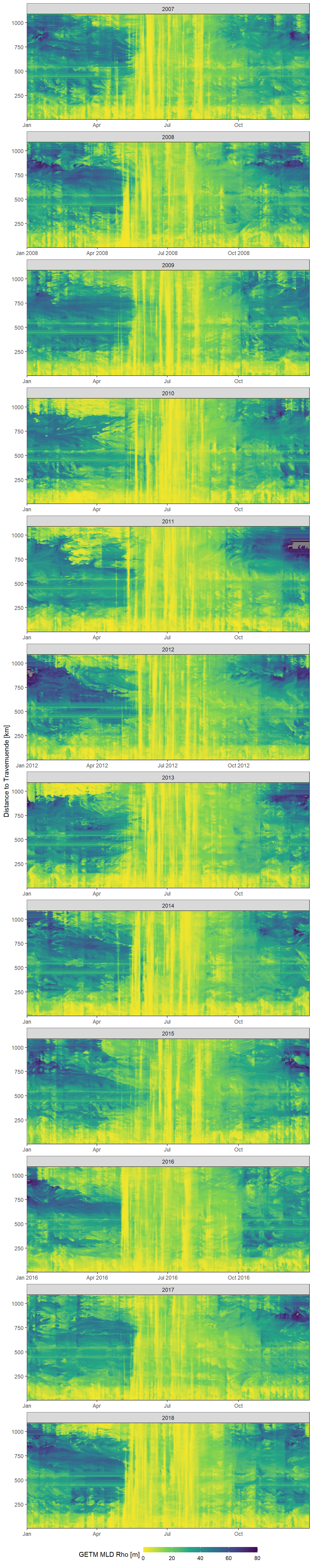
Daily mean GETM mld rho values as a function of time and the ships distance to Travemuende along route E.
This timeseries represents mixed layer depth values for the parameter mld_tke from 2007 to 2019.
#mld tke
# there are negative values and values up to ~3000, therefore the second filter (filter(value_mldtke >0, value_mldtke < 300)) was added

ts_mld_pco2_hov %>%
  filter(year > 2006, year < 2019) %>%
  #filter(value_mldtke >0, value_mldtke < 300) %>%
  ggplot()+
    geom_raster(aes(date, dist.trav, fill=value_mldtke))+
      scale_fill_viridis_c(name="GETM MLD Tke [m]",
                           limits = c(0,80),
                           direction = -1)+
      scale_x_date(expand = c(0,0))+
      scale_y_continuous(expand = c(0,0))+
      labs(y="Distance to Travemuende [km]")+
      theme_bw()+
      theme(
        axis.title.x = element_blank(),
        legend.position = "bottom",
        legend.key.width = unit(1.3, "cm"),
        legend.key.height = unit(0.3, "cm")
      )+
      facet_wrap(~year, ncol = 1, scales = "free_x")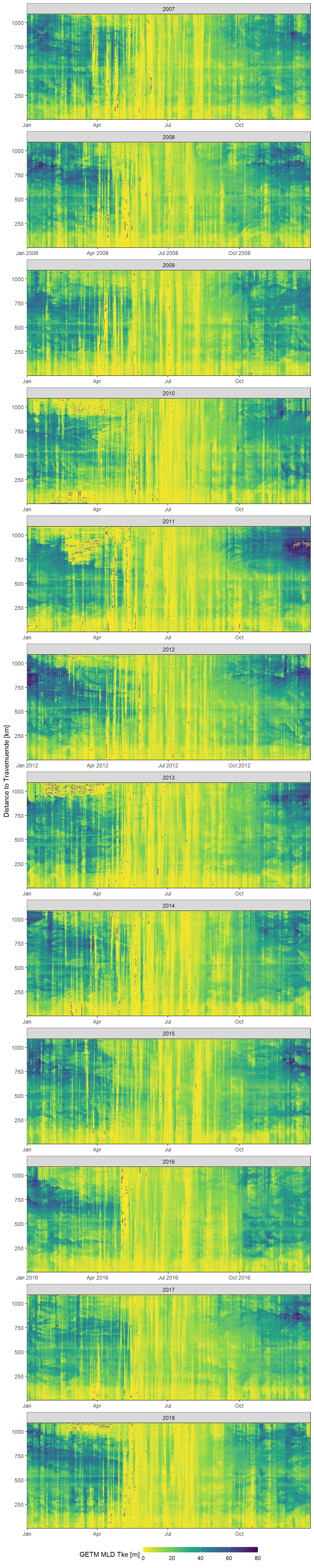
Daily mean GETM mld tke values as a function of time and the ships distance to Travemuende along route E.
###Weekly Finnmaid pCO2 readings
ts_pco2_hov <- ts_mld_pco2_hov %>%
  mutate(date = ymd(date),
         week = as.Date(cut(date, breaks="weeks")),
         dist.trav = corvector*2)

ts_pco2_hov <- ts_pco2_hov %>%
  select(value_pCO2_Finn, week, dist.trav) %>%
  dplyr::group_by(dist.trav, week) %>%
  summarise_all(list(mean=~mean(.,na.rm=TRUE))) %>%
  as.data.frame() %>%
  mutate(year = year(week),
  value_pco2_Finn_mean = mean)


ts_pco2_hov %>%
  filter(year > 2006, year < 2019) %>%
    ggplot()+
    geom_raster(aes(week, dist.trav, fill=value_pco2_Finn_mean))+
    #scale_fill_scico(palette = "vik", name="mean difference in SST [°C]")+
    scale_fill_viridis_c(name="Finnmaid pCO2 [ppm]",
                         limits = c(50,600),
                         na.value = "white")+
    scale_x_date(expand = c(0,0))+
    scale_y_continuous(expand = c(0,0))+
    labs(y="Distance to Travemuende [km]")+
    theme_bw()+
    theme(
      axis.title.x = element_blank(),
      legend.position = "bottom",
      legend.key.width = unit(1.3, "cm"),
      legend.key.height = unit(0.3, "cm")
    )+
    facet_wrap(~year, ncol = 1, scales = "free_x")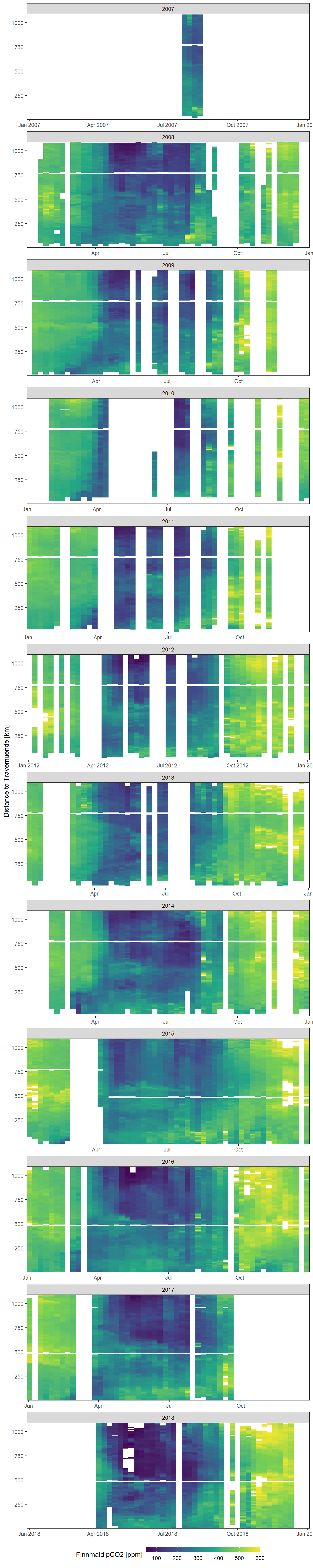
Mean weekly observed (Finnmaid) pCO2 as a function of time and the ships distance to Travemuende along route E.
2.4.2 Comparison pCO2 and mld age 5
ts_mld_pco2_hov <- ts_mld_pco2_hov %>%
  mutate(date = ymd(date),
         week = as.Date(cut(date, breaks="weeks")),
         dist.trav = corvector*2)

comparison_ts_mld_pco2_hov <- ts_mld_pco2_hov %>%
  mutate(relation = (value_pCO2_Finn/value_mld5)) %>%
  select(relation, week, dist.trav) %>%
  dplyr::group_by(dist.trav, week) %>%
  summarise_all(list(relation=~mean(., na.rm = TRUE))) %>%
  as.data.frame %>%
  mutate(year = year(week))

comparison_ts_mld_pco2_hov %>%
  dplyr::filter(year > 2006, year < 2019) %>%
    ggplot()+
    geom_raster(aes(week, dist.trav, fill= relation))+
    scale_fill_viridis_c(name="pCO2 / MLD [ppm/m]",
                         limits = c(0,50),
                         na.value = "white")+
    scale_x_date(expand = c(0,0))+
    scale_y_continuous(expand = c(0,0))+
    labs(y="Distance to Travemuende [km]")+
    theme_bw()+
    theme(
      axis.title.x = element_blank(),
      legend.position = "bottom",
      legend.key.width = unit(1.3, "cm"),
      legend.key.height = unit(0.3, "cm")
    )+
    facet_wrap(~year, ncol = 1, scales = "free_x")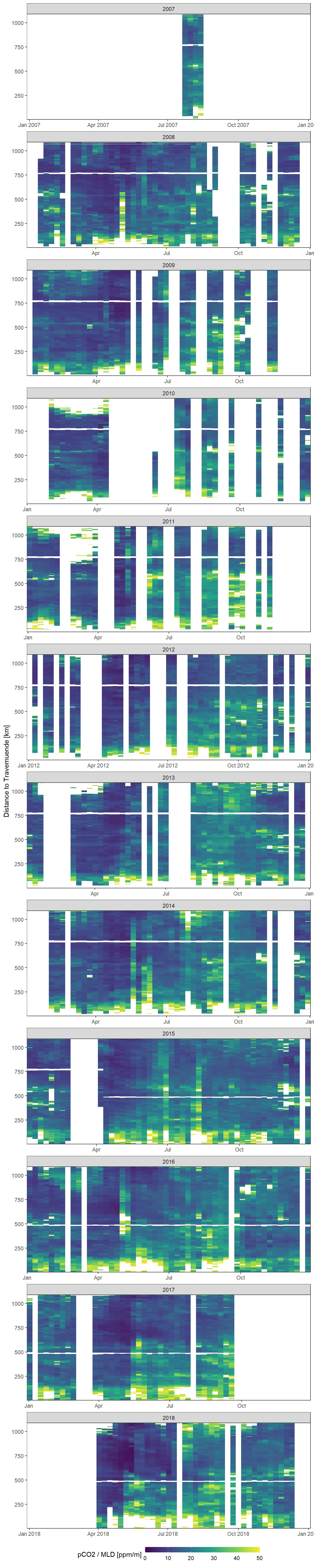
Mean weekly ratio between modelled (GETM) mixed layer depth and observed (Finnmaid) pCO2 values as a function of time and the ships distance to Travemuende along route E.
rm(ts_pco2_hov, comparison_ts_mld_pco2_hov, ts_mld_pco2_hov)
sessionInfo()R version 3.5.0 (2018-04-23)
Platform: x86_64-w64-mingw32/x64 (64-bit)
Running under: Windows 10 x64 (build 18363)
Matrix products: default
locale:
[1] LC_COLLATE=English_United States.1252
[2] LC_CTYPE=English_United States.1252
[3] LC_MONETARY=English_United States.1252
[4] LC_NUMERIC=C
[5] LC_TIME=English_United States.1252
attached base packages:
[1] stats graphics grDevices utils datasets methods base
other attached packages:
[1] metR_0.5.0 here_0.1 xts_0.11-2 zoo_1.8-6
[5] dygraphs_1.1.1.6 geosphere_1.5-10 lubridate_1.7.4 vroom_1.2.0
[9] ncdf4_1.17 forcats_0.4.0 stringr_1.4.0 dplyr_0.8.3
[13] purrr_0.3.3 readr_1.3.1 tidyr_1.0.0 tibble_2.1.3
[17] ggplot2_3.3.0 tidyverse_1.3.0
loaded via a namespace (and not attached):
[1] nlme_3.1-137 bitops_1.0-6 fs_1.3.1
[4] bit64_0.9-7 httr_1.4.1 rprojroot_1.3-2
[7] tools_3.5.0 backports_1.1.5 R6_2.4.0
[10] DBI_1.0.0 colorspace_1.4-1 withr_2.1.2
[13] sp_1.3-2 tidyselect_0.2.5 gridExtra_2.3
[16] bit_1.1-14 compiler_3.5.0 git2r_0.26.1
[19] cli_1.1.0 rvest_0.3.5 xml2_1.2.2
[22] labeling_0.3 scales_1.0.0 checkmate_1.9.4
[25] digest_0.6.22 foreign_0.8-70 rmarkdown_2.0
[28] pkgconfig_2.0.3 htmltools_0.4.0 highr_0.8
[31] dbplyr_1.4.2 maps_3.3.0 htmlwidgets_1.5.1
[34] rlang_0.4.5 readxl_1.3.1 rstudioapi_0.10
[37] generics_0.0.2 jsonlite_1.6 RCurl_1.95-4.12
[40] magrittr_1.5 Formula_1.2-3 dotCall64_1.0-0
[43] Matrix_1.2-14 Rcpp_1.0.2 munsell_0.5.0
[46] lifecycle_0.1.0 stringi_1.4.3 yaml_2.2.0
[49] plyr_1.8.4 grid_3.5.0 maptools_0.9-8
[52] formula.tools_1.7.1 parallel_3.5.0 promises_1.1.0
[55] crayon_1.3.4 lattice_0.20-35 haven_2.2.0
[58] hms_0.5.2 zeallot_0.1.0 knitr_1.26
[61] pillar_1.4.2 reprex_0.3.0 glue_1.3.1
[64] evaluate_0.14 data.table_1.12.6 modelr_0.1.5
[67] operator.tools_1.6.3 vctrs_0.2.0 spam_2.3-0.2
[70] httpuv_1.5.2 cellranger_1.1.0 gtable_0.3.0
[73] assertthat_0.2.1 xfun_0.10 broom_0.5.3
[76] later_1.0.0 viridisLite_0.3.0 memoise_1.1.0
[79] fields_9.9 workflowr_1.6.0