Data base
Jens Daniel Müller
17 March, 2020
Last updated: 2020-03-17
Checks: 6 1
Knit directory: BloomSail/
This reproducible R Markdown analysis was created with workflowr (version 1.6.0). The Checks tab describes the reproducibility checks that were applied when the results were created. The Past versions tab lists the development history.
Great! Since the R Markdown file has been committed to the Git repository, you know the exact version of the code that produced these results.
Great job! The global environment was empty. Objects defined in the global environment can affect the analysis in your R Markdown file in unknown ways. For reproduciblity it’s best to always run the code in an empty environment.
The command set.seed(20191021) was run prior to running the code in the R Markdown file. Setting a seed ensures that any results that rely on randomness, e.g. subsampling or permutations, are reproducible.
Great job! Recording the operating system, R version, and package versions is critical for reproducibility.
Nice! There were no cached chunks for this analysis, so you can be confident that you successfully produced the results during this run.
Using absolute paths to the files within your workflowr project makes it difficult for you and others to run your code on a different machine. Change the absolute path(s) below to the suggested relative path(s) to make your code more reproducible.
| absolute | relative |
|---|---|
| C:/Mueller_Jens_Data/Research/Projects/BloomSail/data/TinaV/Sensor/Profiles_Transects | data/TinaV/Sensor/Profiles_Transects |
| C:/Mueller_Jens_Data/Research/Projects/BloomSail/ | . |
| C:/Mueller_Jens_Data/Research/Projects/BloomSail/data/TinaV/Sensor/Ostergarnsholm | data/TinaV/Sensor/Ostergarnsholm |
| C:/Mueller_Jens_Data/Research/Projects/BloomSail/data/TinaV/Track/GPS_Logger_Track | data/TinaV/Track/GPS_Logger_Track |
Great! You are using Git for version control. Tracking code development and connecting the code version to the results is critical for reproducibility. The version displayed above was the version of the Git repository at the time these results were generated.
Note that you need to be careful to ensure that all relevant files for the analysis have been committed to Git prior to generating the results (you can use wflow_publish or wflow_git_commit). workflowr only checks the R Markdown file, but you know if there are other scripts or data files that it depends on. Below is the status of the Git repository when the results were generated:
Ignored files:
    Ignored:    .Rhistory
    Ignored:    .Rproj.user/
    Ignored:    data/Maps/
    Ignored:    data/Ostergarnsholm/
    Ignored:    data/TinaV/
    Ignored:    data/_merged_data_files/
    Ignored:    data/_summarized_data_files/
Note that any generated files, e.g. HTML, png, CSS, etc., are not included in this status report because it is ok for generated content to have uncommitted changes.
There are no past versions. Publish this analysis with wflow_publish() to start tracking its development.
library(tidyverse)
library(data.table)
library(lubridate)
library(DataExplorer)
library(leaflet)
CTD Sensor data
Regular profiles and transects
CTD sensor data including recordings from auxiliary pH, O2, Chla and pCO2 sensors were recorded with a measurement frequency of 15 sec. (In addition, pCO2 data were also internally recorded on the Contros HydroC instrument with higher temporal resolution and will later be used for further analysis after merging with CTD data.)
setwd("C:/Mueller_Jens_Data/Research/Projects/BloomSail/data/TinaV/Sensor/Profiles_Transects")
files <- list.files(pattern = "[.]cnv$")
#file <- files[1]

for (file in files){

  start.date <- data.table(read.delim(file, sep="#", nrows = 160))[[78,1]]
  start.date <- substr(start.date, 15, 34)
  start.date <- mdy_hms(start.date, tz="UTC")

  tempo <- read.delim(file, sep="", skip = 160, header = FALSE)
  tempo <- data.table(tempo[,c(2,3,4,5,6,7,9,11,13)])
  names(tempo) <- c("date", "Dep.S", "Tem.S", "Sal.S", "V_pH", "pH", "Chl", "O2", "pCO2")
  tempo$start.date <- start.date
  tempo$date <- tempo$date + tempo$start.date

  tempo$transect.ID <- substr(file, 1, 6)
  tempo$type <- substr(file, 8,8)
  tempo$label <- substr(file, 8,10)

  tempo$cast <- "up"
  tempo[date < mean(tempo[Dep.S == max(tempo$Dep.S)]$date)]$cast <- "down"

  if (exists("dataset")){
    dataset <- rbind(dataset, tempo)
  }

  if (!exists("dataset")){
    dataset <- tempo
  }

  rm(start.date)
  rm(tempo)
}


CTD <- dataset
rm(dataset, file, files)


setwd("C:/Mueller_Jens_Data/Research/Projects/BloomSail/")
setwd("C:/Mueller_Jens_Data/Research/Projects/BloomSail/data/TinaV/Sensor/Ostergarnsholm")
files <- list.files(pattern = "[.]cnv$")
#file <- files[1]
for (file in files){
start.date <- data.table(read.delim(file, sep="#", nrows = 160))[[78,1]]
start.date <- substr(start.date, 15, 34)
start.date <- mdy_hms(start.date, tz="UTC")
tempo <- read.delim(file, sep="", skip = 160, header = FALSE)
tempo <- data.table(tempo[,c(2,3,4,5,6,7,9,11,13)])
names(tempo) <- c("date", "Dep.S", "Tem.S", "Sal.S", "V_pH", "pH", "Chl", "O2", "pCO2")
tempo$start.date <- start.date
tempo$date <- tempo$date + tempo$start.date
tempo$transect.ID <- substr(file, 1, 6)
tempo$type <- substr(file, 8,8)
tempo$label <- substr(file, 11,12)
tempo$cast <- "up"
tempo[date < mean(tempo[Dep.S == max(tempo$Dep.S)]$date)]$cast <- "down"
if (exists("dataset")){
dataset <- rbind(dataset, tempo)
}
if (!exists("dataset")){
dataset <- tempo
}
rm(start.date)
rm(tempo)
}
OGB <- dataset
rm(dataset, file, files)
OGB <- OGB %>%
mutate(type = if_else(label=="bo", "P", "T"),
label = if_else(label == "bo", "P14", label),
label = if_else(label == "in", "T14", label),
label = if_else(label == "ou", "T15", label))
setwd("C:/Mueller_Jens_Data/Research/Projects/BloomSail/")CTD <- bind_rows(CTD, OGB) %>%
arrange(date)
rm(OGB)source("code/eda.R")
eda(CTD, "CTD-raw")
rm(eda)The output of an automated Exploratory Data Analysis (EDA) performed with the package DataExplorer can be accessed here:
Link to EDA report of CTD raw data
CTD recordings were cleaned from obviously erroneous readings, by setting values to NA.
class(CTD)
CTD <- data.table(CTD)

# Profiling data

# Temperature

# CTD %>%
#   filter(type == "P") %>%
#   ggplot(aes(Tem.S, Dep.S, col=label, linetype = cast))+
#   geom_line()+
#   scale_y_reverse()+
#   geom_vline(xintercept = c(10, 20))+
#   facet_wrap(~transect.ID)

CTD[transect.ID == "180723" & label == "P07" & Dep.S < 2 & cast == "up"]$Tem.S <- NA

# Salinity

# CTD %>%
#   filter(type == "P") %>%
#   ggplot(aes(Sal.S, Dep.S, col=label, linetype = cast))+
#   geom_path()+
#   scale_y_reverse()+
#   facet_wrap(~transect.ID)

CTD[Sal.S < 6]$Sal.S <- NA

# pH

# CTD %>%
#   filter(type == "P") %>%
#   ggplot(aes(pH, Dep.S, col=label, linetype=cast))+
#   geom_path()+
#   scale_y_reverse()+
#   facet_wrap(~transect.ID)
#
# CTD %>%
#   filter(type == "P") %>%
#   ggplot(aes(V_pH, Dep.S, col=label, linetype=cast))+
#   geom_path()+
#   scale_y_reverse()+
#   facet_wrap(~transect.ID)

CTD[pH < 7.5]$V_pH <- NA
CTD[pH < 7.5]$pH <- NA

CTD[transect.ID == "180709" & label == "P03" & Dep.S < 5 & cast == "down"]$pH <- NA
CTD[transect.ID == "180709" & label == "P05" & Dep.S < 10 & cast == "down"]$pH <- NA
CTD[transect.ID == "180718" & label == "P10" & Dep.S < 3 & cast == "down"]$pH <- NA
CTD[transect.ID == "180815" & label == "P03" & Dep.S < 2 & cast == "down"]$pH <- NA
CTD[transect.ID == "180820" & label == "P11" & Dep.S < 15 & cast == "down"]$pH <- NA

CTD[transect.ID == "180709" & label == "P03" & Dep.S < 5 & cast == "down"]$V_pH <- NA
CTD[transect.ID == "180709" & label == "P05" & Dep.S < 10 & cast == "down"]$V_pH <- NA
CTD[transect.ID == "180718" & label == "P10" & Dep.S < 3 & cast == "down"]$V_pH <- NA
CTD[transect.ID == "180815" & label == "P03" & Dep.S < 2 & cast == "down"]$V_pH <- NA
CTD[transect.ID == "180820" & label == "P11" & Dep.S < 15 & cast == "down"]$V_pH <- NA


# pCO2

# CTD %>%
#   filter(type == "P") %>%
#   ggplot(aes(pCO2, Dep.S, col=label, linetype = cast))+
#   geom_path()+
#   scale_y_reverse()+
#   facet_wrap(~transect.ID)

CTD[transect.ID == "180616"]$pCO2 <- NA

# O2

# CTD %>%
#   filter(type == "P") %>%
#   ggplot(aes(O2, Dep.S, col=label, linetype = cast))+
#   geom_path()+
#   scale_y_reverse()+
#   facet_wrap(~transect.ID)

# Chlorophyll

# CTD %>%
#   filter(type == "P") %>%
#   ggplot(aes(Chl, Dep.S, col=label, linetype = cast))+
#   geom_path()+
#   scale_y_reverse()+
#   facet_wrap(~transect.ID)

CTD[Chl > 100]$Chl <- NA


#### Surface transect data

# CTD %>%
#   filter(type == "T") %>%
#   ggplot(aes(date, Dep.S, col=label))+
#   geom_point()+
#   scale_y_reverse()+
#   facet_wrap(~transect.ID, scales = "free_x")
#
# CTD %>%
#   filter(type == "T") %>%
#   ggplot(aes(date, Tem.S, col=label))+
#   geom_point()+
#   facet_wrap(~transect.ID, scales = "free_x")
#
# CTD %>%
#   filter(type == "T") %>%
#   ggplot(aes(date, Sal.S, col=label))+
#   geom_point()+
#   facet_wrap(~transect.ID, scales = "free_x")
#
# CTD %>%
#   filter(type == "T") %>%
#   ggplot(aes(date, pCO2, col=label))+
#   geom_point()+
#   facet_wrap(~transect.ID, scales = "free_x")
#
# CTD %>%
#   filter(type == "T") %>%
#   ggplot(aes(date, pH, col=label))+
#   geom_point()+
#   facet_wrap(~transect.ID, scales = "free_x")
#
# CTD %>%
#   filter(type == "T") %>%
#   ggplot(aes(date, Chl, col=label))+
#   geom_point()+
#   facet_wrap(~transect.ID, scales = "free_x")

CTD[type == "T" & Chl > 10]$Chl <- NA


# CTD %>%
#   filter(type == "T") %>%
#   ggplot(aes(date, O2, col=label))+
#   geom_point()+
#   facet_wrap(~transect.ID, scales = "free_x")
Relevant columns were selected and renamed, only observations from regular stations (P01-P13) and transects (T01-T13) were selected and summarized data were written to file.
CTD <-
  CTD %>%
  select(date_time=date,
         ID=transect.ID,
         type,
         station=label,
         dep=Dep.S,
         sal=Sal.S,
         tem=Tem.S,
         pCO2,pH,V_pH,O2,Chl)

# CTD <- CTD %>%
#   filter( !(station %in% c("PX1", "PX2", "TX1", "TX2") ))

CTD %>%
  write_csv(here::here("data/_summarized_data_files", "Tina_V_Sensor_Profiles_Transects.csv"))

rm(CTD)
CTD <-
read_csv(here::here("data/_summarized_data_files", "Tina_V_Sensor_Profiles_Transects.csv"),
col_types = cols(pCO2 = col_double()))source("code/eda.R")
eda(CTD, "CTD")
rm(eda)The output of an automated Exploratory Data Analysis (EDA) performed with the package DataExplorer can be accessed here:
Link to EDA report of CTD clean data
CTD %>%
  arrange(date_time) %>%
  filter(type == "P", !(station %in% c("PX1", "PX2"))) %>%
  ggplot(aes(tem, dep, col=station))+
  geom_path()+
  scale_y_reverse()+
  labs(x="Temperature (°C)", y="Depth (m)")+
  facet_wrap(~ID, labeller = label_both)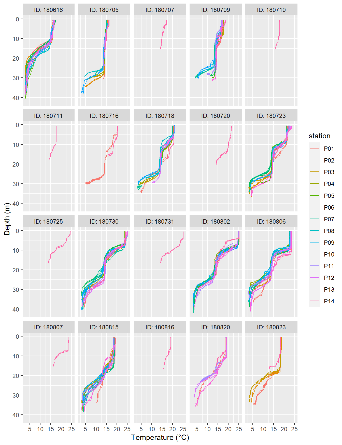
Temperature profiles recorded on regular stations P01-P13. ID refers to the starting date of each cruise.
CTD %>%
  arrange(date_time) %>%
  filter(type == "P", !(station %in% c("PX1", "PX2"))) %>%
  ggplot(aes(pCO2, dep, col=station))+
  geom_path()+
  scale_y_reverse()+
  labs(x=expression(pCO[2]~(µatm)), y="Depth (m)")+
  facet_wrap(~ID, labeller = label_both)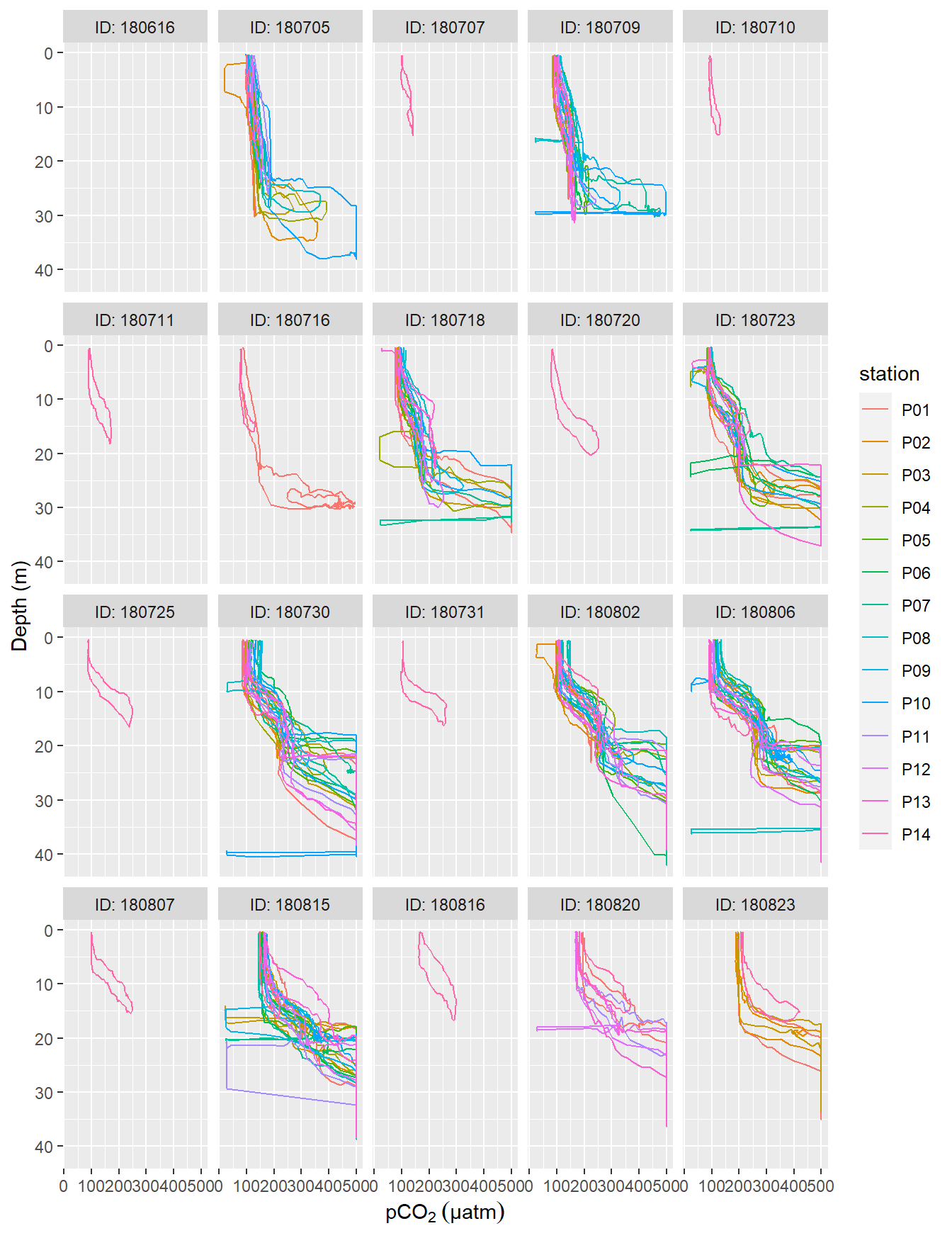
pCO2 profiles (analog output from HydroC) recorded on regular stations P01-P13. ID refers to the starting date of each cruise. Please note that pCO2 measurement range is restricted to 100-500 µatm here due to the settings of the analog voltage output of the sensor. Zeroing periods are included.
pCO2 data
HydroC pCO2 data were provided by KM Contros after applying a drift correction to the raw data, which was based on pre- and post-deployment calibration results.
# Read Contros corrected data file

HC <-
  read_csv2(here::here("Data/TinaV/Sensor/HydroC-pCO2/corrected_Contros",
                       "parameter&pCO2s(method 43).txt"),
            col_names = c("date_time", "Zero", "Flush", "p_NDIR",
                          "p_in", "T_control", "T_gas", "%rH_gas",
                          "Signal_raw", "Signal_ref", "T_sensor",
                          "pCO2", "Runtime", "nr.ave")) %>%
  mutate(date_time = dmy_hms(date_time),
         Flush = as.factor(as.character(Flush)),
         Zero = as.factor(as.character(Zero)))
Individual deployments (periods of observations with less than 30 sec between recordings) were identified and relevant deployment periods were subsetted.
HC <- HC %>%
  arrange(date_time) %>%
  mutate(deployment = cumsum(c(TRUE,diff(date_time)>=30)))

HC <- HC %>%
  filter(deployment %in% c(2,6,9,14,17,21,23,27,31,33,34,35,37))
# add counter for date_time observations
HC <- HC %>%
add_count(date_time)
# find triplicated time stamp and select only first observation, and merge
HC_no_triple <- HC %>%
filter(n <= 2)
HC_triple_clean <- HC %>%
filter(n > 2) %>%
slice(1)
HC <- full_join(HC_no_triple, HC_triple_clean)
rm(list=setdiff(ls(), "HC"))
# find duplicated time stamps and shift first by one second backward, and merge
HC %>%
distinct(date_time)
HC <- HC %>%
select(-n) %>%
add_count(date_time)
unique(HC$n)
HC_no_duplicated <- HC %>%
filter(n == 1)
HC_duplicated <- HC %>%
filter(n == 2)
HC_duplicated_first <- HC_duplicated %>%
group_by(date_time) %>%
slice(1) %>%
ungroup() %>%
mutate(date_time = date_time - 1)
HC_duplicated_second <- HC_duplicated %>%
group_by(date_time) %>%
slice(2) %>%
ungroup()
HC_duplicated_clean <- full_join(HC_duplicated_first, HC_duplicated_second) %>%
arrange(date_time)
HC <- full_join(HC_no_duplicated, HC_duplicated_clean)
HC %>%
distinct(date_time)
rm(list=setdiff(ls(), "HC"))
# find duplicated time stamps and shift first by two seconds forward, and merge
HC %>%
distinct(date_time)
HC <- HC %>%
select(-n) %>%
add_count(date_time)
unique(HC$n)
HC_no_duplicated <- HC %>%
filter(n == 1)
HC_duplicated <- HC %>%
filter(n == 2)
HC_duplicated_first <- HC_duplicated %>%
group_by(date_time) %>%
slice(1) %>%
ungroup() %>%
mutate(date_time = date_time + 2)
HC_duplicated_second <- HC_duplicated %>%
group_by(date_time) %>%
slice(2) %>%
ungroup()
HC_duplicated_clean <- full_join(HC_duplicated_first, HC_duplicated_second) %>%
arrange(date_time)
HC <- full_join(HC_no_duplicated, HC_duplicated_clean)
HC %>%
distinct(date_time)
rm(list=setdiff(ls(), "HC"))
# remaining duplicates are observations where other observations with a +/- 1 sec timestamp exist
# for those cases, only the first duplicated observation is selected (similar to triplicate treatment)
HC %>%
distinct(date_time)
HC <- HC %>%
select(-n) %>%
add_count(date_time)
unique(HC$n)
HC_still_no_duplicated <- HC %>%
filter(n == 1)
HC_still_duplicated_first <- HC %>%
filter(n == 2) %>%
group_by(date_time) %>%
slice(1)
HC <- full_join(HC_still_no_duplicated, HC_still_duplicated_first)
HC %>%
distinct(date_time)
rm(list=setdiff(ls(), "HC"))
HC <- HC %>%
select(-n)# Zeroing ID labelling
HC <- HC %>%
arrange(date_time) %>%
group_by(Zero) %>%
mutate(Zero_ID = as.factor(cumsum(c(TRUE,diff(date_time)>=30)))) %>%
ungroup()
unique(HC$Zero_ID)
# Flush: Identification
HC <- HC %>%
mutate(Flush = 0) %>%
group_by(Zero, Zero_ID) %>%
mutate(start = min(date_time),
duration = date_time - start,
Flush = if_else(Zero == 0 & duration < 600, "1", "0")) %>%
ungroup()
# Flush: Identify equilibration and internal gas mixing periods
HC <- HC %>%
mutate(mixing = if_else(duration < 20, "mixing", "equilibration"))A pdf with plots of all Flush periods (mixing and equilibration identified) can be found here:
pdf(file=here::here("output/Plots/data_base",
    "HydroC_pCO2_deployments.pdf"), onefile = TRUE, width = 7, height = 4)

for (i in unique(HC$deployment)) {

  #i <- unique(HC$deployment)[3]

  sub <-  HC %>%
      filter(deployment == i)
  start_date <- min(sub$date_time)

  print(
    sub %>%
      ggplot(aes(date_time, pCO2, col=Zero_ID))+
      geom_line()+
      labs(title = paste("Deployment: ",i, "| Start time: ", start_date))
)

}

dev.off()

rm(sub, start_date, i)
A pdf with pCO2 timeseries plots of all deployments can be found here:
source("code/eda.R")
eda(HC, "HydroC-pCO2")
rm(eda)
The output of an automated Exploratory Data Analysis (EDA) performed with the package DataExplorer can be accessed here:
Link to EDA report of HydroC pCO2 data data
Individual zeroings were labeled with a counter and a period of 10 min after the zeroing was labelled as Flush period (overriding the internal Flush flag). A mixing flag was introduced, flagging the initial 20 sec of each Flush period as “mixing” and the rest as “equilibration”.
Flush <- HC %>%
 filter(Flush == 1)

# Flush: Plot individual periods

pdf(file=here::here("output/Plots/data_base",
    "Flush_periods_all.pdf"), onefile = TRUE, width = 7, height = 4)

for (i in unique(Flush$Zero_ID)) {

  #i <- unique(Flush$Zero_ID)[5]
print(
  Flush %>%
    filter(Zero_ID == i) %>%
    ggplot(aes(duration, pCO2, col=mixing))+
    geom_point() +
    scale_color_brewer(palette = "Set1")+
    labs(y=expression(pCO[2]~(µatm)), x="Duration of Flush period (s)",
             title = paste("Zero_ID: ", i))
)

}

dev.off()

rm(Flush,i)
Summarized pCO2 date were written to file.
HC %>%
  write_csv(here::here("Data/_summarized_data_files",
                       "Tina_V_HydroC_full.csv"))

HC %>%
  select(date_time, Zero, Flush, pCO2, deployment, Zero_ID, duration, mixing) %>%
  write_csv(here::here("Data/_summarized_data_files",
                       "Tina_V_HydroC.csv"))
Bottle data
CO2
Bottle <- read_csv(here::here("Data/TinaV/Bottle/Tracegases", "BloomSail_bottle_CO2_all.csv"),
                   col_types = list("c","c","n","n","n","n","n"))

Bottle <- Bottle %>%
  select(ID=transect.ID,
         station=label,
         dep=Dep,
         sal=Sal,
         CT, AT,
         pH_Mosley = pH.Mosley)

Bottle %>%
  write_csv(here::here("Data/_summarized_data_files", "Tina_V_Bottle_CO2_lab.csv"))
GPS Track
First, we read the GPS track data.
setwd("C:/Mueller_Jens_Data/Research/Projects/BloomSail/data/TinaV/Track/GPS_Logger_Track")
files <- list.files(pattern = "[.]txt$")


for (file in files){

  # if the merged dataset does exist, append to it
  if (exists("dataset")){

    tempo<-data.table ( read.delim(file, sep=",")[,c(2,3,4)])
    names(tempo) <- c("date_time", "lat", "lon")
    tempo$date_time<- ymd_hms(tempo$date, tz="UTC")

    dataset<-rbind(dataset, tempo)
    rm(tempo)
  }

  # if the merged dataset doesn't exist, create it
  if (!exists("dataset")){
    dataset<-data.table ( read.delim(file, sep=",")[,c(2,3,4)])
    names(dataset) <- c("date_time", "lat", "lon")
    dataset$date_time<- ymd_hms(dataset$date_time, tz="UTC")

  }
}

track <- dataset
rm(dataset, file, files)

setwd("C:/Mueller_Jens_Data/Research/Projects/BloomSail")

track %>%
  write_csv(here::here("Data/_summarized_data_files",
                       "TinaV_Track.csv"))

# track_sub <- track %>%
#  slice(which(row_number() %% 20 == 1))
#
# bathy <- read_csv(here::here("data/Maps","Bathymetry_Gotland_east.csv"))
#
# track_sub %>%
#   ggplot()+
#   geom_raster(data=bathy, aes(lon, lat, fill=elev))+
#   scale_fill_continuous(na.value = "black", name="Tiefe [m]")+
#   geom_path(aes(lon, lat), col="grey80")+
#   labs(x="Längengrad (°E)", y="Breitengrad (°N)")+
#   coord_quickmap(expand = 0, ylim = c(57.25,57.6), xlim = c(18.6, 19.8))+
#   theme_bw()+
#   guides(col = guide_legend(nrow = 5))
And than create an interactive map.
track <-
  read_csv(here::here("Data/_summarized_data_files",
                       "TinaV_Track.csv"))

track_sub <- track %>%
  slice(which(row_number() %% 20 == 1))

rm(track)

leaflet() %>%
  setView(lng = 20, lat = 57.3, zoom = 8) %>%
  addLayersControl(baseGroups = c("Ocean Basemap",
                                  "Satellite"),
                   overlayGroups = c("Track"),
                   options = layersControlOptions(collapsed = FALSE),
                   position = 'topright') %>%
  addProviderTiles("Esri.WorldImagery", group = "Satellite") %>%
  addProviderTiles(providers$Esri.OceanBasemap, group = "Ocean Basemap") %>%
  addScaleBar(position = 'topright') %>%
  addMeasure(
    primaryLengthUnit = "kilometers",
    secondaryLengthUnit = 'miles',
    primaryAreaUnit = "sqmeters",
    secondaryAreaUnit="acres",
    position = 'topleft') %>%
  addPolylines(data = track_sub, ~lon, ~lat,
               color = "red",
               group = "Track")
Tasks / open questions
Include data from crossing large vessels
Include information about HydroC calibration results and raw data correction by Contros
Check results from field response time experiment (high zeroing frequency)
sessionInfo()R version 3.5.0 (2018-04-23)
Platform: x86_64-w64-mingw32/x64 (64-bit)
Running under: Windows 10 x64 (build 18363)
Matrix products: default
locale:
[1] LC_COLLATE=English_United States.1252
[2] LC_CTYPE=English_United States.1252
[3] LC_MONETARY=English_United States.1252
[4] LC_NUMERIC=C
[5] LC_TIME=English_United States.1252
attached base packages:
[1] stats graphics grDevices utils datasets methods base
other attached packages:
[1] leaflet_2.0.2 DataExplorer_0.8.0 lubridate_1.7.4 data.table_1.12.6
[5] forcats_0.4.0 stringr_1.4.0 dplyr_0.8.3 purrr_0.3.3
[9] readr_1.3.1 tidyr_1.0.0 tibble_2.1.3 ggplot2_3.3.0
[13] tidyverse_1.3.0
loaded via a namespace (and not attached):
[1] Rcpp_1.0.2 here_0.1 lattice_0.20-35 assertthat_0.2.1
[5] zeallot_0.1.0 rprojroot_1.3-2 digest_0.6.22 mime_0.7
[9] R6_2.4.0 cellranger_1.1.0 backports_1.1.5 reprex_0.3.0
[13] evaluate_0.14 httr_1.4.1 highr_0.8 pillar_1.4.2
[17] rlang_0.4.5 readxl_1.3.1 rstudioapi_0.10 rmarkdown_2.0
[21] labeling_0.3 htmlwidgets_1.5.1 igraph_1.2.4.1 munsell_0.5.0
[25] shiny_1.4.0 broom_0.5.3 compiler_3.5.0 httpuv_1.5.2
[29] modelr_0.1.5 xfun_0.10 pkgconfig_2.0.3 htmltools_0.4.0
[33] tidyselect_0.2.5 gridExtra_2.3 workflowr_1.6.0 crayon_1.3.4
[37] dbplyr_1.4.2 withr_2.1.2 later_1.0.0 grid_3.5.0
[41] xtable_1.8-4 nlme_3.1-137 jsonlite_1.6 gtable_0.3.0
[45] lifecycle_0.1.0 DBI_1.0.0 git2r_0.26.1 magrittr_1.5
[49] scales_1.0.0 cli_1.1.0 stringi_1.4.3 fs_1.3.1
[53] promises_1.1.0 xml2_1.2.2 generics_0.0.2 vctrs_0.2.0
[57] tools_3.5.0 glue_1.3.1 crosstalk_1.0.0 hms_0.5.2
[61] networkD3_0.4 fastmap_1.0.1 parallel_3.5.0 yaml_2.2.0
[65] colorspace_1.4-1 rvest_0.3.5 knitr_1.26 haven_2.2.0