CT dynamics
Jens Daniel Müller
20 March, 2020
Last updated: 2020-03-20
Checks: 7 0
Knit directory: BloomSail/
This reproducible R Markdown analysis was created with workflowr (version 1.6.0). The Checks tab describes the reproducibility checks that were applied when the results were created. The Past versions tab lists the development history.
Great! Since the R Markdown file has been committed to the Git repository, you know the exact version of the code that produced these results.
Great job! The global environment was empty. Objects defined in the global environment can affect the analysis in your R Markdown file in unknown ways. For reproduciblity it’s best to always run the code in an empty environment.
The command set.seed(20191021) was run prior to running the code in the R Markdown file. Setting a seed ensures that any results that rely on randomness, e.g. subsampling or permutations, are reproducible.
Great job! Recording the operating system, R version, and package versions is critical for reproducibility.
Nice! There were no cached chunks for this analysis, so you can be confident that you successfully produced the results during this run.
Great job! Using relative paths to the files within your workflowr project makes it easier to run your code on other machines.
Great! You are using Git for version control. Tracking code development and connecting the code version to the results is critical for reproducibility. The version displayed above was the version of the Git repository at the time these results were generated.
Note that you need to be careful to ensure that all relevant files for the analysis have been committed to Git prior to generating the results (you can use wflow_publish or wflow_git_commit). workflowr only checks the R Markdown file, but you know if there are other scripts or data files that it depends on. Below is the status of the Git repository when the results were generated:
Ignored files:
    Ignored:    .Rhistory
    Ignored:    .Rproj.user/
    Ignored:    data/Finnmaid_2018/
    Ignored:    data/Maps/
    Ignored:    data/Ostergarnsholm/
    Ignored:    data/TinaV/
    Ignored:    data/_merged_data_files/
    Ignored:    data/_summarized_data_files/

Untracked files:
    Untracked:  analysis/BloomSail_surface.Rmd

Unstaged changes:
    Deleted:    analysis/Reconstruction.Rmd
    Modified:   analysis/_site.yml
Note that any generated files, e.g. HTML, png, CSS, etc., are not included in this status report because it is ok for generated content to have uncommitted changes.
There are no past versions. Publish this analysis with wflow_publish() to start tracking its development.
library(tidyverse)
library(patchwork)
library(seacarb)
library(metR)
library(scico)
library(cmocean)
# library(broom)
# library(lubridate)
# library(tibbletime)
1 Sensor data
Profile data are prepared by:
- Ignoring those made on June 16 (pCO2 sensor not in operation)
- Removing HydroC Flush and Zeroing periods
- Selecting only continous downcast periods
- Gridding profiles to 1m depth intervals
- Discarding profiles with 3 or more observation missing within upper 20m
- assigning mean date_time value to all profiles belonging to one cruise
- discarding “coastal” station P01, P13, P14
1.1 pCO2 profile overview
df <-
 read_csv(here::here("data/_merged_data_files",
                      "BloomSail_CTD_HydroC_track_RT.csv"),
               col_types = cols(ID = col_character(),
                                pCO2_analog = col_double(),
                                pCO2 = col_double(),
                                Zero = col_character(),
                                Flush = col_character(),
                                mixing = col_character(),
                                Zero_ID = col_integer(),
                                deployment = col_integer(),
                                lon = col_double(),
                                lat = col_double(),
                                pCO2_RT = col_double()))


# Filter relevant rows and columns

df <- df %>%
  filter(type == "P",
         Flush == "0",
         Zero == "0",
         !ID %in% c("180616","180820"),
         !(station %in% c("PX1", "PX2", "P14", "P13", "P01"))) %>%
  select(date_time, ID, type, station, lat, lon, dep, sal, tem, pCO2_raw = pCO2, pCO2 = pCO2_RT_mean, duration)


# Assign meta information

df <- df %>%
  group_by(ID, station) %>%
  mutate(duration = as.numeric(date_time - min(date_time))) %>%
  arrange(date_time) %>%
  ungroup()

meta <- read_csv(here::here("Data/_summarized_data_files",
                          "Tina_V_Sensor_meta.csv"),
                 col_types = cols(ID = col_character()))

meta <- meta %>%
    filter(!ID %in% c("180616","180820"),
           !(station %in% c("PX1", "PX2", "P14", "P13", "P01")))

df <- full_join(df, meta)
rm(meta)


# creating descriptive variables
df <- df %>%
  mutate(phase = "standby",
         phase = if_else(duration >= start & duration < down & !is.na(down) & !is.na(start),   "down", phase),
         phase = if_else(duration >= down  & duration < lift & !is.na(lift) & !is.na(down ),   "low",  phase),
         phase = if_else(duration >= lift  & duration < up   & !is.na(up  ) & !is.na(lift  ),  "mid",  phase),
         phase = if_else(duration >= up    & duration < end  & !is.na(end ) & !is.na(up   ),   "up",   phase))

df <- df %>%
  select(-c(start, down, lift, up, end, comment, p_type, duration, type))


# select downcasst only
df <- df %>%
  filter(phase == "down") %>%
  select(-phase)


df_highres <- df

# grid observation to 1m depth intervals
df <- df %>%
  mutate(dep_int = as.numeric(as.character( cut(dep, seq(0,40,1), seq(0.5,39.5,1))))) %>%
  group_by(ID, station, dep_int) %>%
  summarise_all("mean", na.rm = TRUE) %>%
  ungroup() %>%
  select(-dep, dep=dep_int)

# subset complete profiles
profiles_in <- df %>%
  filter(dep < 20) %>%
  group_by(ID, station) %>%
  summarise(nr = n()) %>%
  mutate(select = if_else(nr > 18 | station == "P14", "in", "out")) %>%
  select(-nr) %>%
  ungroup()

df <- full_join(df, profiles_in)
rm(profiles_in)

df %>%
  filter(dep < 30) %>%
  arrange(date_time) %>%
  ggplot(aes(pCO2, dep, col=select))+
  geom_point()+
  geom_path()+
  scale_y_reverse()+
  scale_x_continuous(breaks = c(0,300), labels = c(0,300))+
  scale_color_brewer(palette = "Set1", direction = -1)+
  coord_cartesian(xlim = c(0,400))+
  facet_grid(ID~station)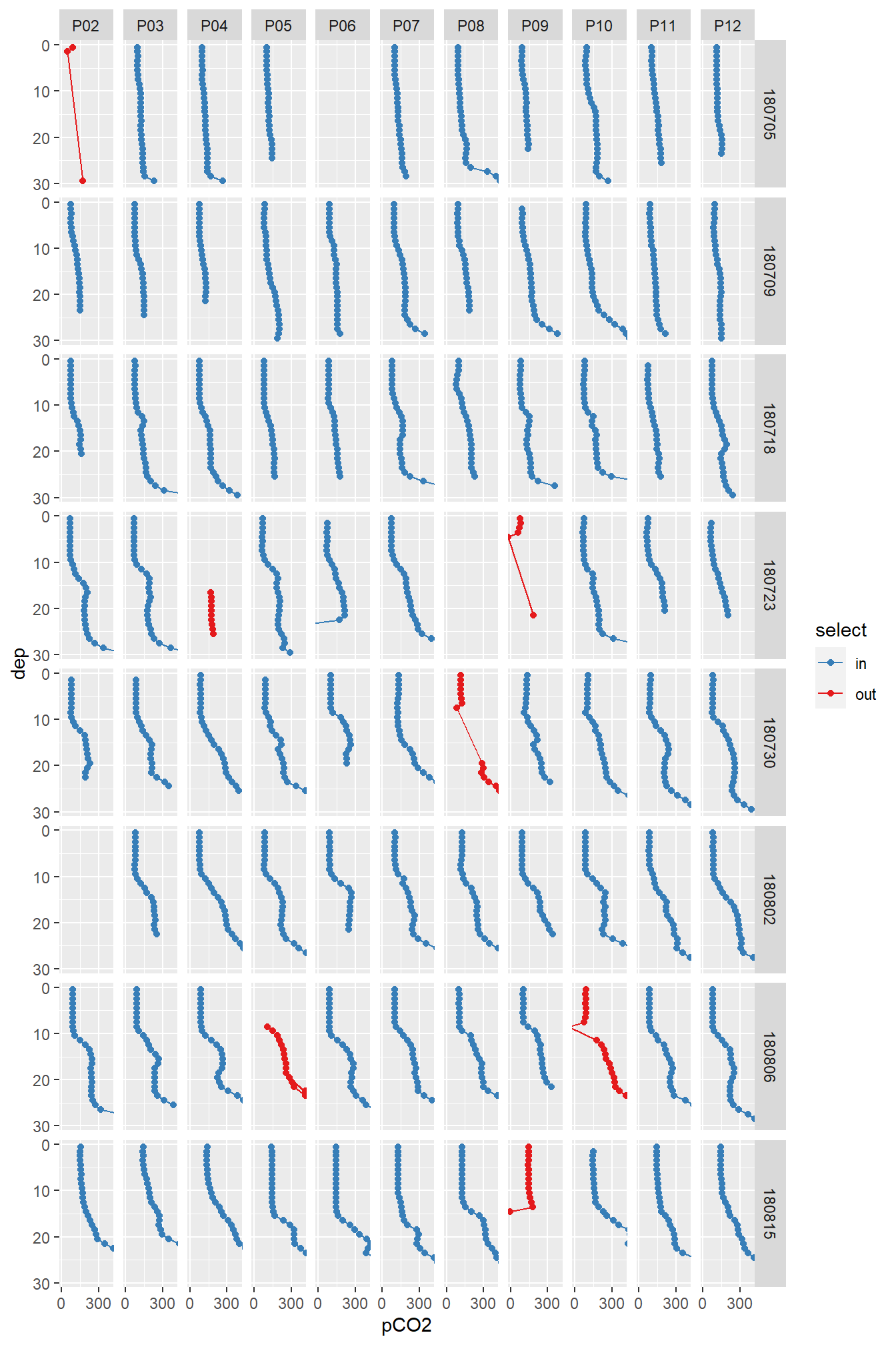
Overview pCO2 profiles at stations (P01-P14) and cruise dates (ID)
df <- df %>%
  filter(select == "in") %>%
  select(-select)

# assign mean date_time stamp

cruise_dates <- df %>%
  filter(station != "P14") %>%
  group_by(ID) %>%
  summarise(date_time_ID = mean(date_time)) %>%
  ungroup()


# inner_join remove P14 observations lacking date_time_ID
df <- inner_join(cruise_dates, df)
1.2 Station map
map <- read_csv(here::here("data/Maps","Bathymetry_Gotland_east_small.csv"))

# ggplot()+
#   geom_contour_fill(data=map, aes(x=lon, y=lat, z=-elev), na.fill = TRUE)+
#   coord_quickmap(expand = 0, xlim = c(18.7, 19.9), ylim = c(57.25,57.6))+
#   theme_bw()+
#   theme(legend.position="bottom")

df %>%
  group_by(station) %>%
  summarise(lat = mean(lat),
            lon = mean(lon)) %>%
  ungroup() %>%
  ggplot()+
  geom_raster(data=map, aes(lon, lat, fill=-elev))+
  scale_fill_scico(palette = "oslo", na.value = "grey",
                   name="Depth [m]", direction = -1)+
  geom_label(aes(lon, lat, label=station))+
  coord_quickmap(expand = 0, xlim = c(18.7, 19.9), ylim = c(57.25,57.6))+
  theme_bw()
Location of stations sampled between the east coast of Gotland and Gotland deep.
rm(map)1.3 Data coverage
cover <- df %>%
  group_by(ID, station) %>%
  summarise(date = mean(date_time),
            date_time_ID = mean(date_time_ID)) %>%
  ungroup()

cover %>%
  ggplot(aes(date, station, fill=ID))+
  geom_vline(aes(xintercept = date_time_ID, col=ID))+
  geom_point(shape=21)+
  scale_color_viridis_d()+
  scale_fill_viridis_d()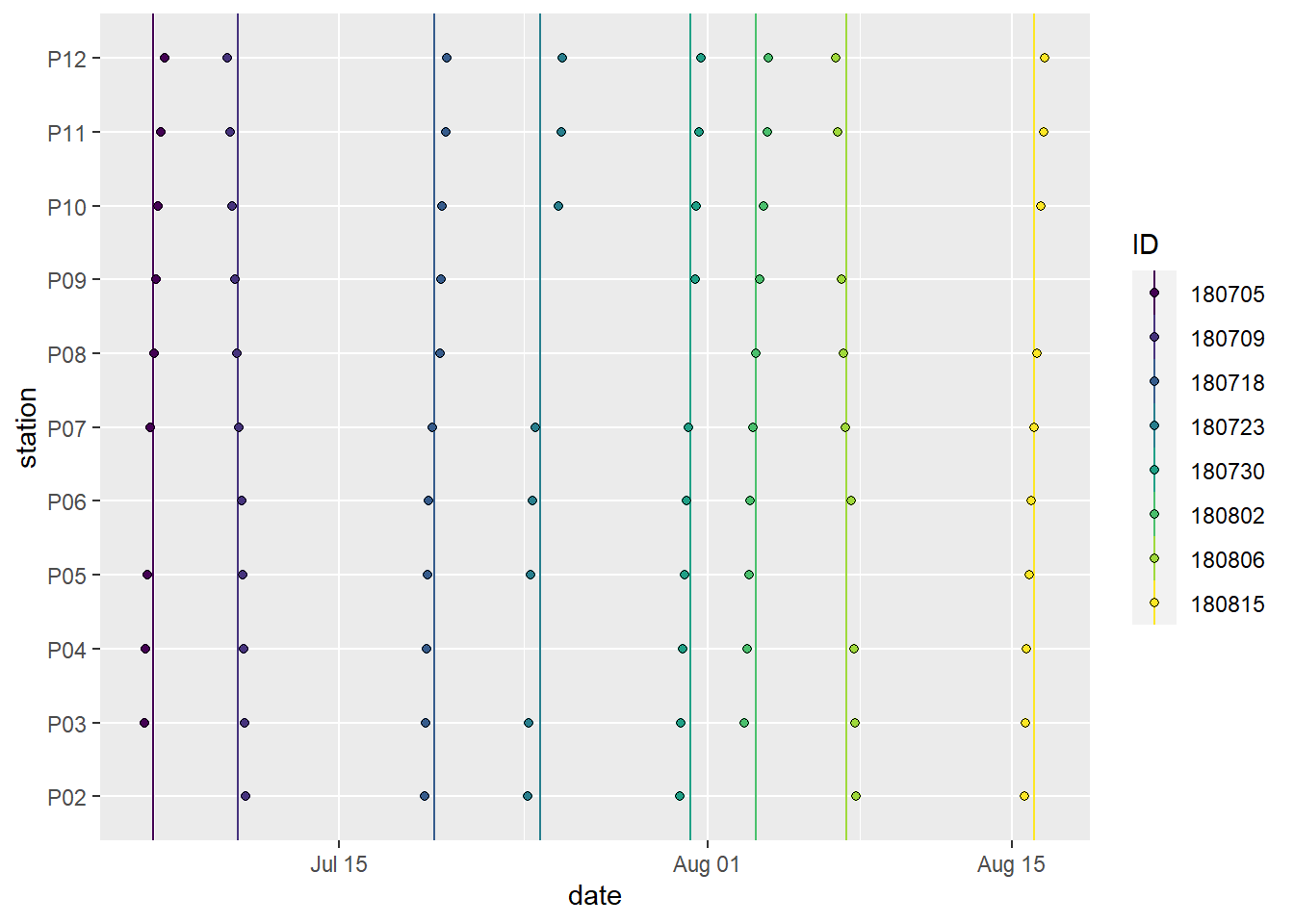
Spatio-temporal data coverage, indicated as station visits over time. ID (color) refers to the starting date of the cruise, except for P14, which was visited twice during each cruise.
rm(cover)2 Bottle CT and AT
At stations P07 and P10 discrete samples for lab measurments of CT and AT were collected. Please note that - in contrast to the pCO2 profiles - samples were taken on June 16.
CO2 <-
  read_csv(here::here("Data/_summarized_data_files", "Tina_V_Bottle_CO2_lab.csv"),
           col_types = cols(ID = col_character()))

CO2 <- CO2 %>%
  filter(station %in% c("P07", "P10")) %>%
  select(-pH_Mosley) %>%
  mutate(CT_AT_ratio = CT/AT)

CO2 <- inner_join(CO2, cruise_dates)
2.1 Vertical profiles
CO2_long <- CO2 %>%
  pivot_longer(4:7, names_to = "parameter", values_to = "value")

CO2_long %>%
  ggplot(aes(value, dep))+
  geom_path(aes(col=ID))+
  geom_point(aes(fill=ID), shape=21)+
  scale_y_reverse()+
  scale_fill_viridis_d()+
  scale_color_viridis_d()+
  facet_grid(station~parameter, scales = "free_x")+
  theme(legend.position = "bottom")
2.2 Surface time series
CO2_ts <- CO2_long %>%
  filter(dep<10) %>%
  group_by(ID, date_time_ID, parameter, station) %>%
  summarise(value = mean(value, na.rm = TRUE)) %>%
  ungroup()

rm(CO2_long)

CO2_ts %>%
  ggplot(aes(date_time_ID, value, col=station))+
  #geom_point(aes(lubridate::ymd(ID), value, col=station))+
  geom_point()+
  geom_path()+
  scale_fill_viridis_d()+
  scale_color_brewer(palette = "Set1")+
  facet_grid(parameter~., scales = "free_y")+
  labs(x="Mean transect date")
Time series of bottle data. Shown are mean values of samples collected at water depths < 10m (usually collected at 0 and 5 m).
AT_mean <- CO2_ts %>%
  filter(parameter == "AT") %>%
  summarise(AT = mean(value, na.rm = TRUE)) %>%
  pull()

CO2_ts %>%
  filter(parameter == "CT_AT_ratio") %>%
  ggplot(aes(lubridate::ymd(ID), value*AT_mean, col=station))+
  geom_point()+
  geom_path()+
  scale_fill_viridis_d()+
  scale_color_brewer(palette = "Set1")+
  labs(x="Mean transect date", y="CT-AT-ratio * mean AT")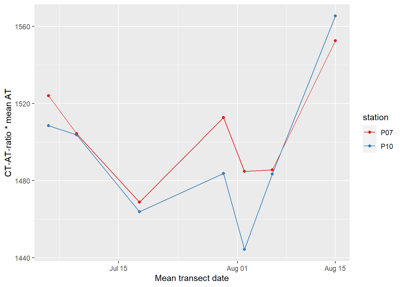
CT timeseries, derived by multiplying the CT-AT-ratio with mean AT
2.3 Mean alkalinity
In order to derive CT from measured pCO2 profiles, the mean alkalinity in the upper 20 m and both stations was calculated as:
AT_mean <- CO2 %>%
  filter(dep <= 20) %>%
  summarise(AT = mean(AT, na.rm = TRUE)) %>%
  pull()

AT_mean
[1] 1717.08Likewise, the mean salinity amounts to:
sal_mean <- CO2 %>%
  filter(dep <= 20) %>%
  summarise(sal = mean(sal, na.rm = TRUE)) %>%
  pull()

sal_mean
[1] 6.8941273 CT profiles
3.1 Calculation from pCO2
CT profiles were calculated from sensor pCO2 and T profiles, and constant salinity and alkalinity values. Note that the impact of fixed vs. measured salinity has only a negligible impact on CT profiles.
df <- df %>%
  drop_na()

df <- df %>%
  filter(pCO2 > 0)

df <- df %>%
  mutate(CT = carb(24, var1=pCO2, var2=1720*1e-6,
                   S=sal_mean, T=tem, P=dep/10, k1k2="m10", kf="dg", ks="d",
                   gas="insitu")[,16]*1e6)

rm(sal_mean, AT_mean)

df %>%
  write_csv(here::here("Data/_merged_data_files", "BloomSail_CTD_HydroC_CT.csv"))
3.2 Mean profiles
Mean vertical profiles were calculated for each cruise day (ID). Note that:
- ID represents the start date of the cruise, not the exact mean sampling date
- Coastal station P14 was excluded so far from the analysis
# df %>%
#   filter(dep < 20) %>%
#   arrange(date_time) %>%
#   ggplot(aes(CT, dep))+
#   geom_point()+
#   geom_path()+
#   scale_y_reverse()+
#   coord_cartesian(ylim = c(30,0))+
#   facet_grid(station~ID)

mean_profiles <- df %>%
  filter(dep < 25) %>%
  select(-c(station,lat, lon, pCO2_raw, date_time)) %>%
  group_by(ID, date_time_ID, dep) %>%
  summarise_all(list(mean), na.rm=TRUE) %>%
  ungroup()

sd_profiles <- df %>%
  filter(dep < 25) %>%
  select(-c(station,lat, lon, pCO2_raw, date_time)) %>%
  group_by(ID, date_time_ID, dep) %>%
  summarise_all(list(sd), na.rm=TRUE) %>%
  ungroup()

sd_profiles_long <- sd_profiles %>%
  pivot_longer(4:7, names_to = "parameter", values_to = "sd")

mean_profiles_long <- mean_profiles %>%
  pivot_longer(4:7, names_to = "parameter", values_to = "value")

mean_profiles_long <- inner_join(mean_profiles_long, sd_profiles_long)

rm(sd_profiles, sd_profiles_long)

mean_profiles_long %>%
  ggplot(aes(value, dep, col=ID))+
  geom_point()+
  geom_path()+
  scale_y_reverse()+
  scale_color_viridis_d()+
  facet_wrap(~parameter, scales = "free_x")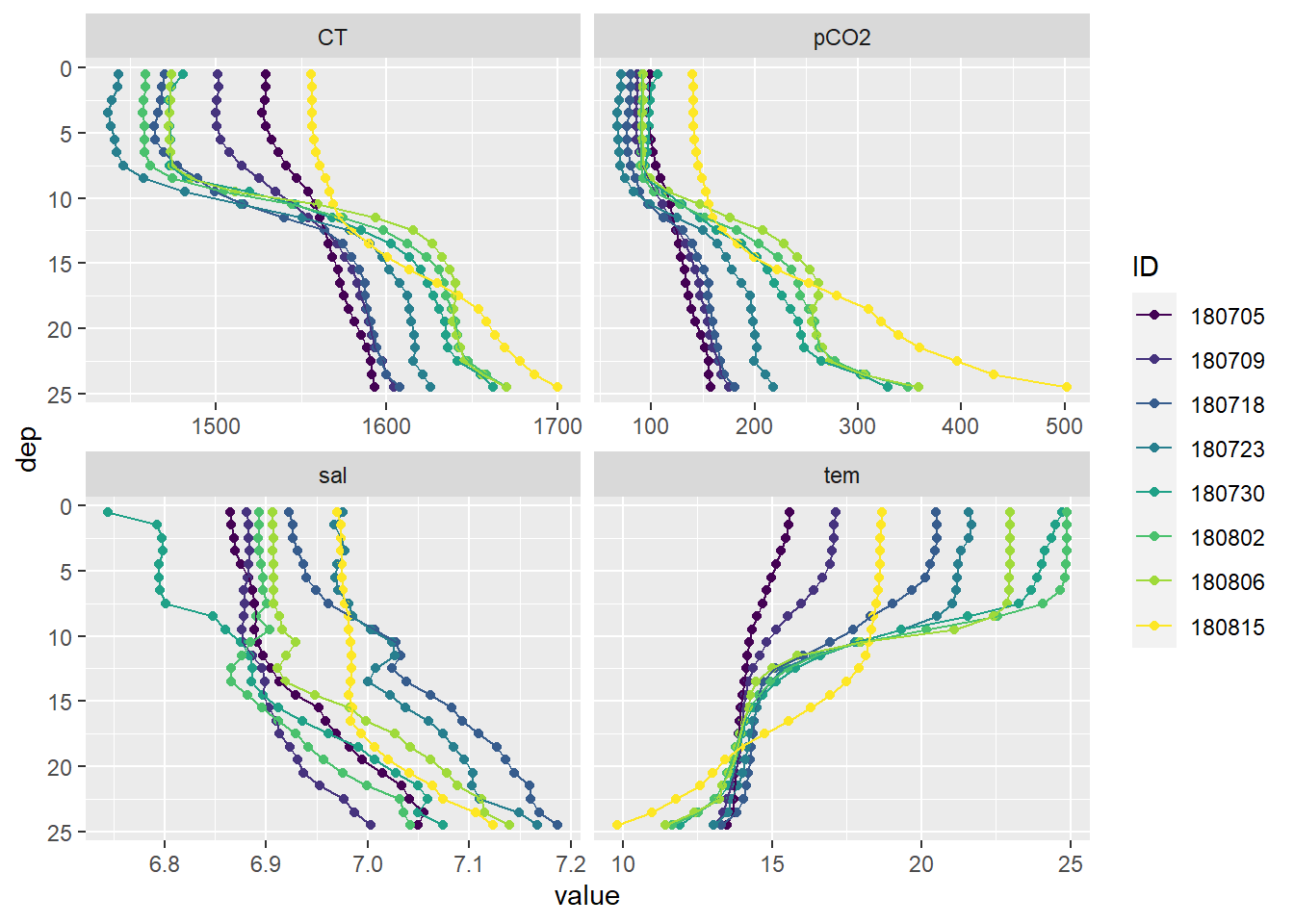
Mean vertical profiles per cruise day across all stations.
all <- mean_profiles_long %>%
  filter(parameter %in% c("CT", "tem")) %>%
  rename(group = ID)

mean_profiles_long %>%
  filter(parameter %in% c("CT", "tem")) %>%
  ggplot()+
  geom_path(data=all, aes(value, dep, group=group))+
  geom_ribbon(aes(xmin = value-sd, xmax=value+sd, y=dep, fill=ID), alpha=0.5)+
  geom_path(aes(value, dep, col=ID))+
  scale_y_reverse()+
  scale_color_viridis_d()+
  scale_fill_viridis_d()+
  facet_grid(ID~parameter, scales = "free_x")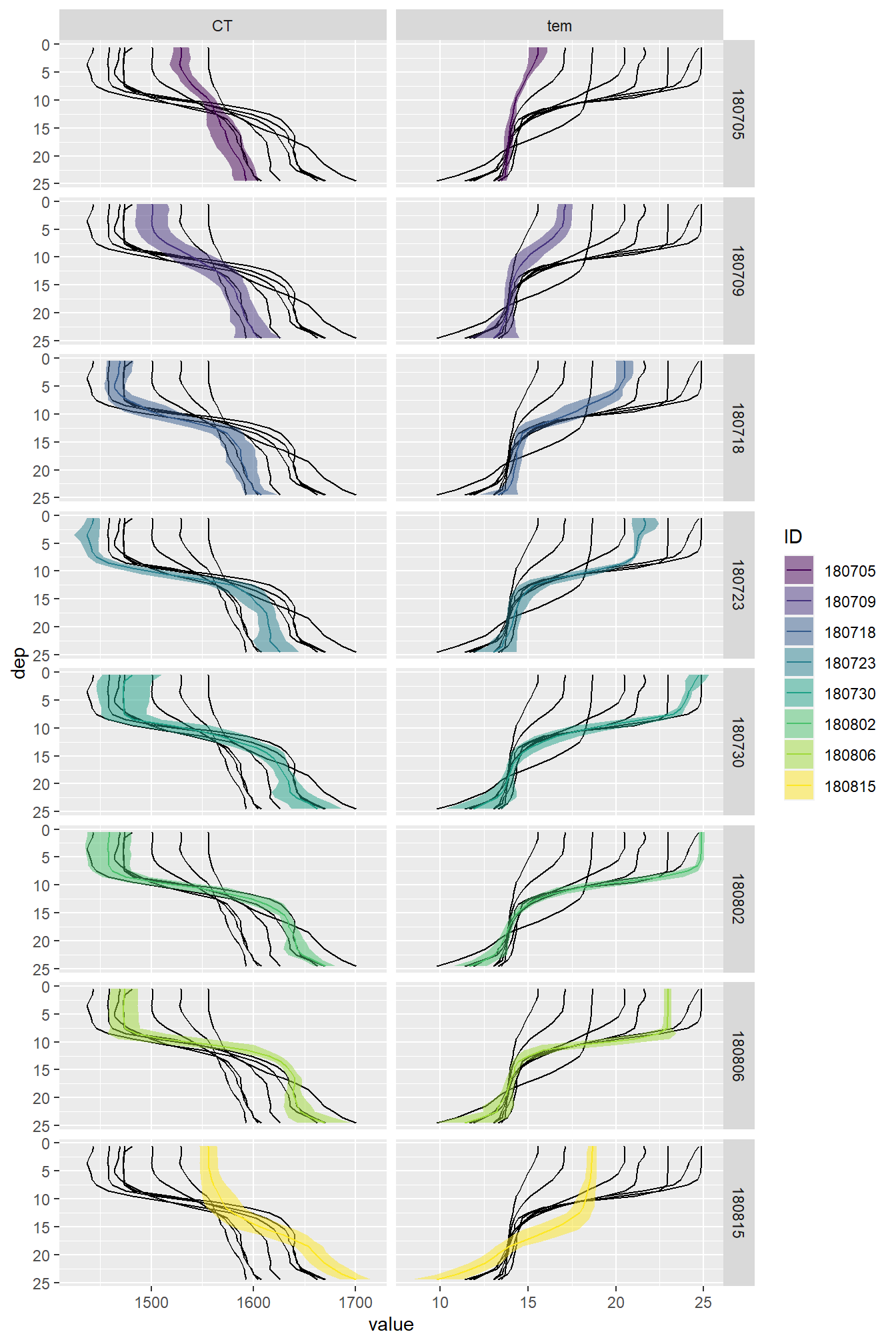
Mean vertical profiles per cruise day across all stations plotted indivdually. Ribbons indicate the standard deviation observed across all profiles at each depth and transect.
3.3 Individual profiles
CT, pCO2, S, and T profiles were plotted individually pdf here and grouped by ID pdf here. The later gives an idea of the differences between stations at one point in time.
pdf(file=here::here("output/Plots/CT_dynamics",
    "profiles_individual.pdf"), onefile = TRUE, width = 9, height = 5)

for(i_ID in unique(df$ID)){
  for(i_station in unique(df$station)){

    if (nrow(df %>% filter(ID == i_ID, station == i_station)) > 0){


      # i_ID      <-      unique(df$ID)[1]
      # i_station <- unique(df$station)[1]

      p_pCO2 <-
        df %>%
        arrange(date_time) %>%
        filter(ID == i_ID,
               station == i_station) %>%
        ggplot(aes(pCO2, dep, col="grid_RT"))+
        geom_point(data = df_highres %>% arrange(date_time) %>% filter(ID == i_ID, station == i_station),
                   aes(pCO2_raw, dep, col="raw"))+
        geom_point(data = df_highres %>% arrange(date_time) %>% filter(ID == i_ID, station == i_station),
                   aes(pCO2, dep, col="raw_RT"))+
        geom_point(aes(pCO2_raw, dep, col="grid"))+
        geom_point()+
        geom_path()+
        scale_y_reverse()+
        scale_color_brewer(palette = "Set1")+
        labs(y="Depth [m]", x="pCO2 [µatm]", title = str_c(i_ID," | ",i_station))+
        coord_cartesian(xlim = c(0,200), ylim = c(30,0))+
        theme_bw()+
        theme(legend.position = "left")

      p_tem <-
        df %>%
        arrange(date_time) %>%
        filter(ID == i_ID,
               station == i_station) %>%
        ggplot(aes(tem, dep))+
        geom_point()+
        geom_path()+
        scale_y_reverse()+
        labs(y="Depth [m]", x="Tem [°C]")+
        coord_cartesian(xlim = c(14,26), ylim = c(30,0))+
        theme_bw()

      p_sal <-
        df %>%
        arrange(date_time) %>%
        filter(ID == i_ID,
               station == i_station) %>%
        ggplot(aes(sal, dep))+
        geom_point()+
        geom_path()+
        scale_y_reverse()+
        labs(y="Depth [m]", x="Tem [°C]")+
        coord_cartesian(xlim = c(6.5,7.5), ylim = c(30,0))+
        theme_bw()

      p_CT <-
        df %>%
        arrange(date_time) %>%
        filter(ID == i_ID,
               station == i_station) %>%
        ggplot(aes(CT, dep))+
        geom_point()+
        geom_path()+
        scale_y_reverse()+
        labs(y="Depth [m]", x="CT* [µmol/kg]")+
        coord_cartesian(xlim = c(1400,1700), ylim = c(30,0))+
        theme_bw()


      print(
            p_pCO2 + p_tem + p_sal + p_CT
            )

      rm(p_pCO2, p_sal, p_tem, p_CT)


    }
  }
}

dev.off()

rm(i_ID, i_station)
df_long <- df %>%
select(-c(lat, lon, pCO2_raw)) %>%
filter(dep < 25) %>%
pivot_longer(6:9, values_to = "value", names_to = "parameter")
pdf(file=here::here("output/Plots/CT_dynamics",
"profiles_by_ID.pdf"), onefile = TRUE, width = 9, height = 5)
for(i_ID in unique(df$ID)){
#i_ID <- unique(df$ID)[1]
sub_df_long <- df_long %>%
arrange(date_time) %>%
filter(ID == i_ID)
print(
sub_df_long %>%
ggplot()+
geom_path(data = df_long, aes(value, dep, group=interaction(station, ID)), col="grey")+
geom_path(aes(value, dep, col=station))+
scale_y_reverse()+
labs(y="Depth [m]", title = str_c("ID: ", i_ID))+
theme_bw()+
facet_wrap(~parameter, scales = "free_x")
)
rm(sub_df_long)
}
dev.off()
rm(i_ID, df_long)3.4 Profiles of incremental changes
Changes of seawater parameters at each depth are calculated from one cruise day to the next and divided by the number of days inbetween.
mean_profiles_long <- mean_profiles_long %>%
    group_by(parameter, dep) %>%
    arrange(date_time_ID) %>%
    mutate(diff_value = value     - lag(value, default = first(value)),
           diff_time  = as.numeric(date_time_ID - lag(date_time_ID)),
           diff_value_daily = diff_value / diff_time,
           cum_value = cumsum(diff_value)) %>%
  ungroup()


mean_profiles_long %>%
  arrange(dep) %>%
  ggplot(aes(diff_value_daily, dep, col=ID))+
  geom_vline(xintercept = 0)+
  geom_point()+
  geom_path()+
  scale_y_reverse()+
  scale_color_viridis_d()+
  facet_wrap(~parameter, scales = "free_x")+
  labs(x="Change of value inbetween cruises per day")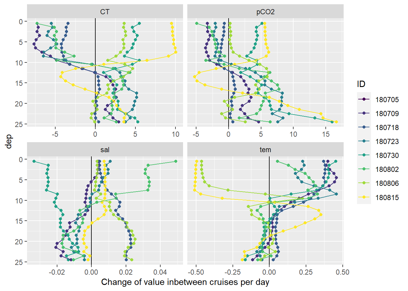
3.5 Profiles of cumulative changes
Cumulative changes of seawater parameters were calculated at each depth relative to the first cruise day on July 5.
mean_profiles_long %>%
  arrange(dep) %>%
  ggplot(aes(cum_value, dep, col=ID))+
  geom_vline(xintercept = 0)+
  geom_point()+
  geom_path()+
  scale_y_reverse()+
  scale_color_viridis_d()+
  facet_wrap(~parameter, scales = "free_x")+
  labs(x="Cumulative change of value")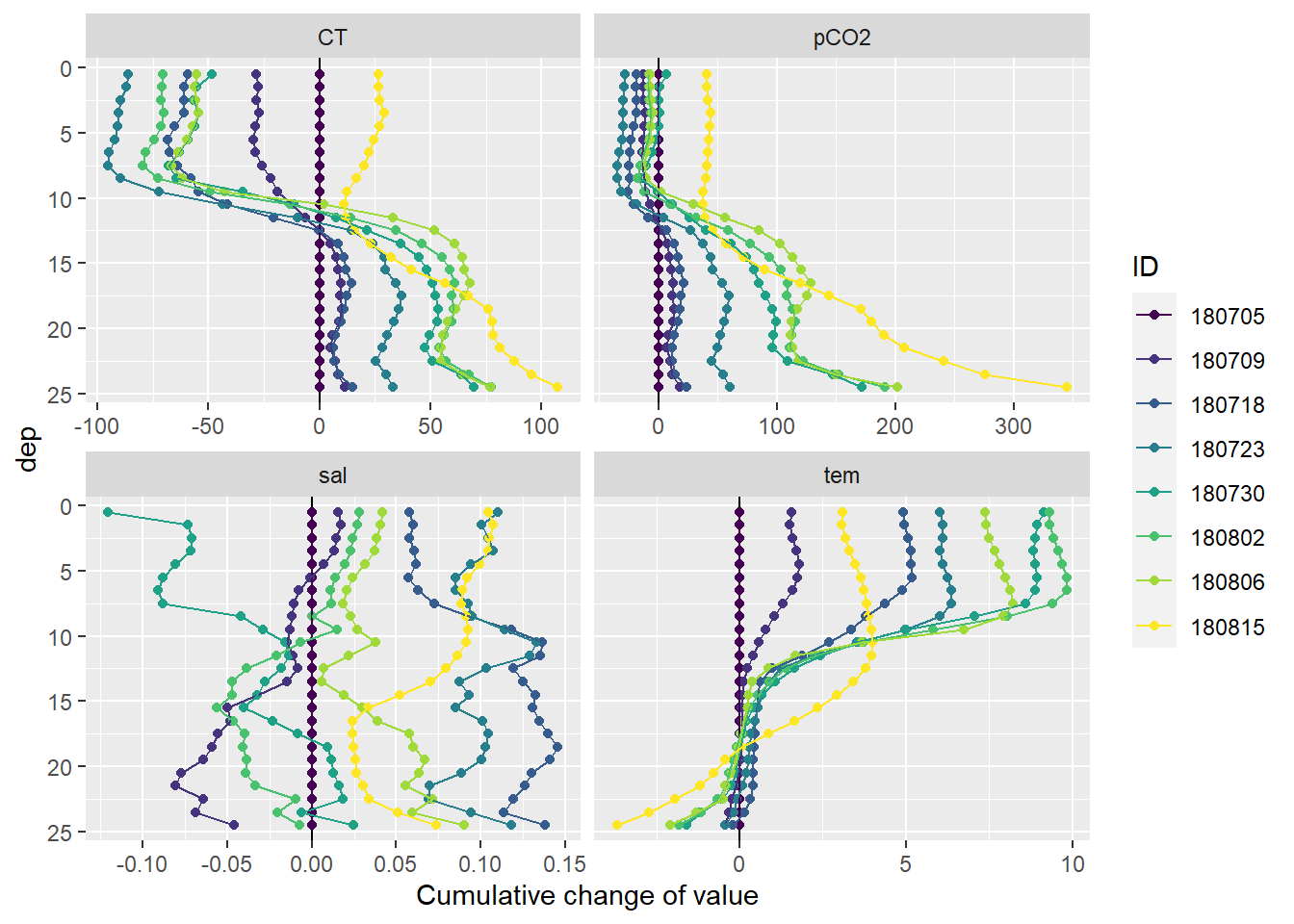
Cumulative positive and negative changes of seawater parameters were calculated separately at each depth relative to the first cruise day on July 5.
mean_profiles_long <- mean_profiles_long %>%
  mutate(sign = if_else(diff_value < 0, "neg", "pos")) %>%
  group_by(parameter, dep, sign) %>%
  arrange(date_time_ID) %>%
  mutate(cum_value_sign = cumsum(diff_value)) %>%
  ungroup()

mean_profiles_long %>%
  write_csv(here::here("Data/_merged_data_files", "BloomSail_CTD_HydroC_CT_cumulative_profiles.csv"))

mean_profiles_long %>%
  arrange(dep) %>%
  ggplot(aes(cum_value_sign, dep, col=ID))+
  geom_vline(xintercept = 0)+
  geom_point()+
  geom_path()+
  scale_y_reverse()+
  scale_color_viridis_d()+
  scale_fill_viridis_d()+
  facet_wrap(~interaction(sign, parameter), scales = "free_x", ncol=4)+
  labs(x="Cumulative directional change of value")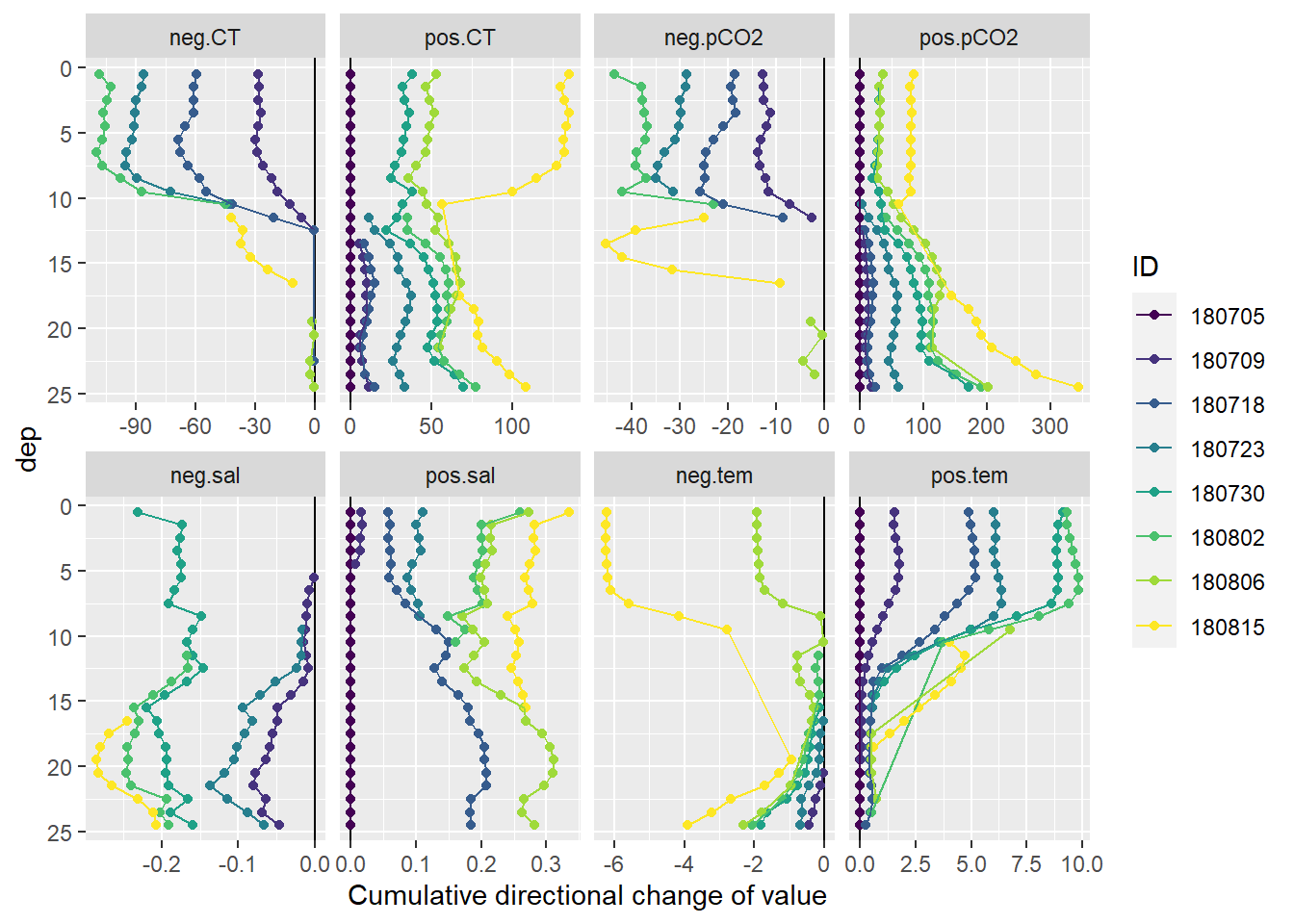
4 Timeseries
4.1 Observed
Timeseries of changes in seawater parameters were calculated for 5m depth intervals.
timeseries <- mean_profiles_long %>%
  mutate(dep = cut(dep, seq(0,30,5))) %>%
  group_by(ID, date_time_ID, dep, parameter)  %>%
  summarise_all(list(mean), na.rm=TRUE)

timeseries %>%
  ggplot(aes(date_time_ID, value, col=as.factor(dep)))+
  geom_path()+
  #geom_errorbar(aes(date_time_ID, ymax=value+sd, ymin=value-sd, col=as.factor(dep)))+
  geom_point()+
  scale_color_viridis_d(name="Depth [m]")+
  facet_wrap(~parameter, scales = "free_y", ncol=1)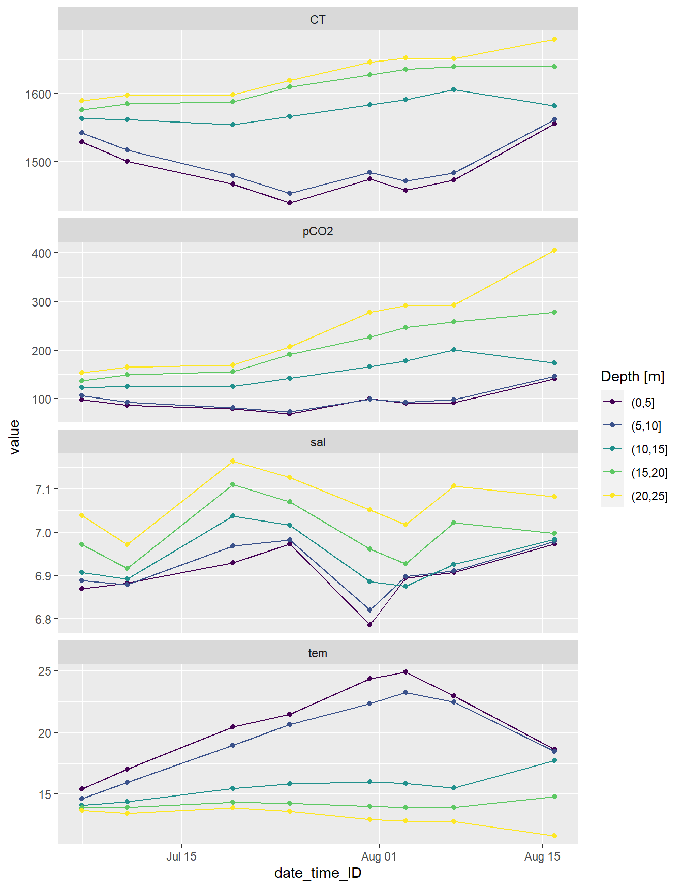
4.2 Incremental and cumulative
Total incremental and cumulative CT changes inbetween cruise dates were calculated for 5m depth intervals.
NCP <- mean_profiles_long %>%
  filter(parameter == "CT") %>%
  mutate(dep = cut(dep, seq(0,30,5))) %>%
  group_by(ID, date_time_ID, dep, sign) %>%
  summarise(dCT = sum(diff_value)/1000) %>%
  ungroup()

NCP <- NCP %>%
  group_by(sign, dep) %>%
  arrange(date_time_ID) %>%
  mutate(dCT_cum = cumsum(dCT)) %>%
  ungroup()

NCP %>%
  write_csv(here::here("Data/_merged_data_files", "BloomSail_CTD_HydroC_CT_cumulative_timeseries.csv"))


NCP_grid <- expand_grid(
  unique(NCP$date_time_ID),
  unique(NCP$dep),
  unique(NCP$sign)
)

NCP_grid <- NCP_grid %>%
  set_names(c("date_time_ID","dep", "sign"))

NCP <- full_join(NCP, NCP_grid)

rm(NCP_grid)

NCP <- NCP %>%
  arrange(sign, dep, date_time_ID) %>%
  group_by(sign, dep) %>%
  fill(dCT_cum) %>%
  ungroup() %>%
  mutate(dCT_cum = if_else(is.na(dCT_cum), 0, dCT_cum))
p_iNCP <- NCP %>%
ggplot(aes(date_time_ID, dCT, fill=dep))+
geom_hline(yintercept = 0)+
geom_bar(stat="identity", col="black")+
scale_fill_viridis_d()+
scale_y_continuous(breaks = seq(-100, 100, 0.2))+
facet_grid(rev(sign)~., scales = "free_y", space = "free_y")+
theme(strip.background = element_blank(),
strip.text = element_blank())+
labs(y="integrated, directional CT changes [mol/m2]", x="date")
p_iNCPcum <- NCP %>%
ggplot(aes(date_time_ID, dCT_cum, fill=dep))+
geom_hline(yintercept = 0)+
geom_area(col="black")+
scale_fill_viridis_d()+
scale_y_continuous(breaks = seq(-100, 100, 0.2))+
facet_grid(rev(sign)~., scales = "free_y", space = "free_y")+
theme(strip.background = element_blank(),
strip.text = element_blank())+
labs(y="integrated, cumulative, directional CT changes [mol/m2]", x="date")
(p_iNCP / p_iNCPcum)+
plot_layout(guides = 'collect')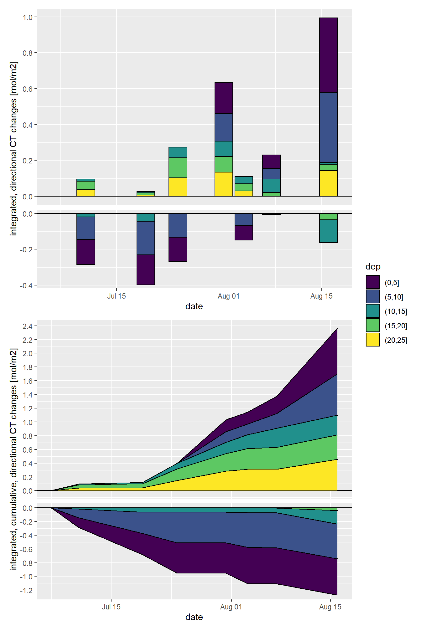
rm(p_iNCP, p_iNCPcum)5 CT vs temperature
As primary production (negative changes in CT) and increase in seawater temperature have a common driver (light), the relation between both changes was investigated.
CT_tem <- mean_profiles %>%
  group_by(dep) %>%
  arrange(date_time_ID) %>%
  mutate(dCT = CT - lag(CT),
         dtem = tem - lag(tem),
         sign = if_else(dCT < 0, "neg", "pos")) %>%
  ungroup() %>%
  drop_na()

CT_tem %>%
  ggplot()+
  geom_hline(yintercept = 0)+
  geom_vline(xintercept = 0)+
  geom_smooth(aes(dtem, dCT), method = "lm", se=FALSE)+
  geom_point(aes(dtem, dCT, fill=ID), shape=21)+
  scale_fill_viridis_d()+
  guides(fill = guide_legend(override.aes=list(shape=21)))
CT_tem %>%
  ggplot(aes(dtem, dCT))+
  geom_hline(yintercept = 0)+
  geom_vline(xintercept = 0)+
  geom_smooth(method = "lm", se=FALSE)+
  geom_point(aes(fill=ID), shape = 21)+
  scale_fill_viridis_d()+
  guides(fill = guide_legend(override.aes=list(shape=21)))+
  facet_wrap(~ID)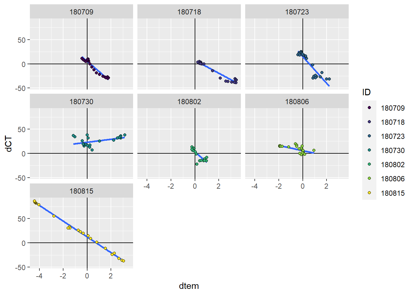
6 Hovmoeller plots
6.1 Absolute values
bin_CT <- 20

CT_hov <- mean_profiles_long %>%
  filter(parameter == "CT") %>%
  ggplot()+
  geom_contour_fill(aes(x=date_time_ID, y=dep, z=value),
                    breaks = MakeBreaks(bin_CT),
                    col="black")+
  geom_point(aes(x=date_time_ID, y=c(24.5)), size=3, shape=24, fill="white")+
  scale_fill_viridis_c(breaks = MakeBreaks(bin_CT),
                       guide = "colorstrip",
                       name="CT (µmol/kg)")+
  scale_y_reverse()+
  theme_bw()+
  labs(y="Depth (m)")+
  coord_cartesian(expand = 0)+
  theme(axis.title.x = element_blank(),
        axis.text.x = element_blank())

bin_Tem <- 2

Tem_hov <- mean_profiles_long %>%
  filter(parameter == "tem") %>%
  ggplot()+
  geom_contour_fill(aes(x=date_time_ID, y=dep, z=value),
                    breaks = MakeBreaks(bin_Tem),
                    col="black")+
  geom_point(aes(x=date_time_ID, y=c(24.5)), size=3, shape=24, fill="white")+
  scale_fill_viridis_c(breaks = MakeBreaks(bin_Tem),
                       guide = "colorstrip",
                       name="Tem (°C)",
                       option = "inferno")+
  scale_y_reverse()+
  theme_bw()+
  labs(x="",y="Depth (m)")+
  coord_cartesian(expand = 0)

CT_hov / Tem_hov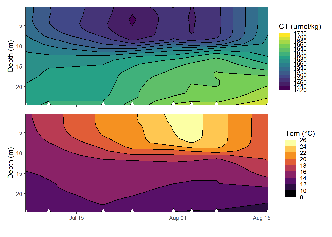
Hovmoeller plots of absolute changes in CT and temperature.
rm(CT_hov, bin_CT, Tem_hov, bin_Tem)6.2 Daily changes
bin_CT <- 2.5

CT_hov <- mean_profiles_long %>%
  filter(parameter == "CT") %>%
  ggplot()+
  geom_contour_fill(aes(x=date_time_ID, y=dep, z=diff_value_daily),
                    breaks = MakeBreaks(bin_CT),
                    col="black")+
  geom_point(aes(x=date_time_ID, y=c(24.5)), size=3, shape=24, fill="white")+
  scale_fill_divergent(breaks = MakeBreaks(bin_CT),
                       guide = "colorstrip",
                       name="CT (µmol/kg)")+
  scale_y_reverse()+
  theme_bw()+
  labs(y="Depth (m)")+
  coord_cartesian(expand = 0)+
  theme(axis.title.x = element_blank(),
        axis.text.x = element_blank())

bin_Tem <- 0.1

Tem_hov <- mean_profiles_long %>%
  filter(parameter == "tem") %>%
  ggplot()+
  geom_contour_fill(aes(x=date_time_ID, y=dep, z=diff_value_daily),
                    breaks = MakeBreaks(bin_Tem),
                    col="black")+
  geom_point(aes(x=date_time_ID, y=c(24.5)), size=3, shape=24, fill="white")+
  scale_fill_divergent(breaks = MakeBreaks(bin_Tem),
                       guide = "colorstrip",
                       name="Tem (°C)")+
  scale_y_reverse()+
  theme_bw()+
  labs(x="",y="Depth (m)")+
  coord_cartesian(expand = 0)

CT_hov / Tem_hov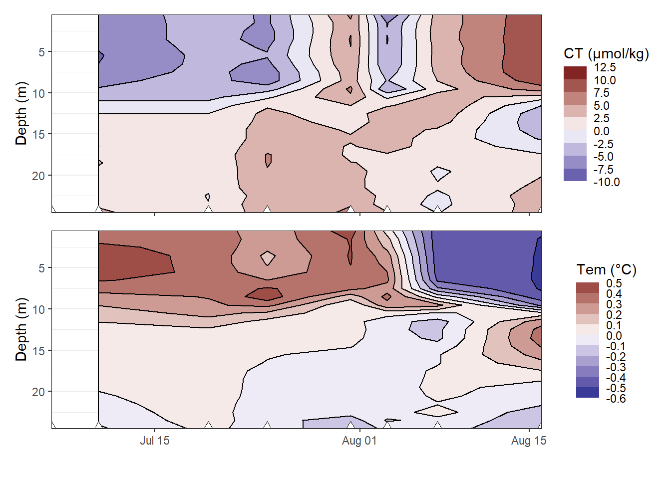
Hovmoeller plots of daily changes in CT and temperature. Note: Daily changes are currently plotted against the day when they were observed compared to the previous transect, although plotting against the mean date would be more plausible.
rm(CT_hov, bin_CT, Tem_hov, bin_Tem)7 Open tasks / questions
- Significance of changes in AT for calculated CT changes
- Harmonize selection of profiles for tau optimization and BGC interpretation (how many missing discrete depth intervals are allowed?)
- refer to mean date between cruises for incremental and cumulative changes?
sessionInfo()R version 3.5.0 (2018-04-23)
Platform: x86_64-w64-mingw32/x64 (64-bit)
Running under: Windows 10 x64 (build 18363)
Matrix products: default
locale:
[1] LC_COLLATE=English_United States.1252
[2] LC_CTYPE=English_United States.1252
[3] LC_MONETARY=English_United States.1252
[4] LC_NUMERIC=C
[5] LC_TIME=English_United States.1252
attached base packages:
[1] stats graphics grDevices utils datasets methods base
other attached packages:
[1] cmocean_0.2 scico_1.1.0 metR_0.5.0 seacarb_3.2.12
[5] oce_1.2-0 gsw_1.0-5 testthat_2.3.1 patchwork_1.0.0
[9] forcats_0.4.0 stringr_1.4.0 dplyr_0.8.3 purrr_0.3.3
[13] readr_1.3.1 tidyr_1.0.0 tibble_2.1.3 ggplot2_3.3.0
[17] tidyverse_1.3.0
loaded via a namespace (and not attached):
[1] nlme_3.1-137 bitops_1.0-6 fs_1.3.1
[4] lubridate_1.7.4 RColorBrewer_1.1-2 httr_1.4.1
[7] rprojroot_1.3-2 tools_3.5.0 backports_1.1.5
[10] R6_2.4.0 mgcv_1.8-23 DBI_1.0.0
[13] colorspace_1.4-1 withr_2.1.2 sp_1.3-2
[16] tidyselect_0.2.5 gridExtra_2.3 compiler_3.5.0
[19] git2r_0.26.1 cli_1.1.0 rvest_0.3.5
[22] xml2_1.2.2 labeling_0.3 scales_1.0.0
[25] checkmate_1.9.4 digest_0.6.22 foreign_0.8-70
[28] rmarkdown_2.0 pkgconfig_2.0.3 htmltools_0.4.0
[31] highr_0.8 dbplyr_1.4.2 maps_3.3.0
[34] rlang_0.4.5 readxl_1.3.1 rstudioapi_0.10
[37] generics_0.0.2 jsonlite_1.6 RCurl_1.95-4.12
[40] magrittr_1.5 Formula_1.2-3 dotCall64_1.0-0
[43] Matrix_1.2-14 Rcpp_1.0.2 munsell_0.5.0
[46] lifecycle_0.1.0 stringi_1.4.3 yaml_2.2.0
[49] plyr_1.8.4 grid_3.5.0 maptools_0.9-8
[52] formula.tools_1.7.1 promises_1.1.0 crayon_1.3.4
[55] lattice_0.20-35 haven_2.2.0 hms_0.5.2
[58] zeallot_0.1.0 knitr_1.26 pillar_1.4.2
[61] reprex_0.3.0 glue_1.3.1 evaluate_0.14
[64] data.table_1.12.6 modelr_0.1.5 operator.tools_1.6.3
[67] vctrs_0.2.0 spam_2.3-0.2 httpuv_1.5.2
[70] cellranger_1.1.0 gtable_0.3.0 assertthat_0.2.1
[73] xfun_0.10 broom_0.5.3 later_1.0.0
[76] viridisLite_0.3.0 memoise_1.1.0 fields_9.9
[79] workflowr_1.6.0 ellipsis_0.3.0 here_0.1