Finnmaid and GETM
Jens Daniel Müller und Lara Sophie Burchardt
21 April, 2020
Last updated: 2020-04-21
Checks: 7 0
Knit directory: BloomSail/
This reproducible R Markdown analysis was created with workflowr (version 1.6.1). The Checks tab describes the reproducibility checks that were applied when the results were created. The Past versions tab lists the development history.
Great! Since the R Markdown file has been committed to the Git repository, you know the exact version of the code that produced these results.
Great job! The global environment was empty. Objects defined in the global environment can affect the analysis in your R Markdown file in unknown ways. For reproduciblity it’s best to always run the code in an empty environment.
The command set.seed(20191021) was run prior to running the code in the R Markdown file. Setting a seed ensures that any results that rely on randomness, e.g. subsampling or permutations, are reproducible.
Great job! Recording the operating system, R version, and package versions is critical for reproducibility.
Nice! There were no cached chunks for this analysis, so you can be confident that you successfully produced the results during this run.
Great job! Using relative paths to the files within your workflowr project makes it easier to run your code on other machines.
Great! You are using Git for version control. Tracking code development and connecting the code version to the results is critical for reproducibility.
The results in this page were generated with repository version a82b4fe. See the Past versions tab to see a history of the changes made to the R Markdown and HTML files.
Note that you need to be careful to ensure that all relevant files for the analysis have been committed to Git prior to generating the results (you can use wflow_publish or wflow_git_commit). workflowr only checks the R Markdown file, but you know if there are other scripts or data files that it depends on. Below is the status of the Git repository when the results were generated:
Ignored files:
    Ignored:    .Rhistory
    Ignored:    .Rproj.user/
    Ignored:    data/Finnmaid_2018/
    Ignored:    data/GETM/
    Ignored:    data/Maps/
    Ignored:    data/Ostergarnsholm/
    Ignored:    data/TinaV/
    Ignored:    data/_merged_data_files/
    Ignored:    data/_summarized_data_files/

Untracked files:
    Untracked:  output/Plots/Figures_publication/

Unstaged changes:
    Deleted:    analysis/license.Rmd
Note that any generated files, e.g. HTML, png, CSS, etc., are not included in this status report because it is ok for generated content to have uncommitted changes.
These are the previous versions of the repository in which changes were made to the R Markdown (analysis/Finnmaid+GETM.Rmd) and HTML (docs/Finnmaid+GETM.html) files. If you’ve configured a remote Git repository (see ?wflow_git_remote), click on the hyperlinks in the table below to view the files as they were in that past version.
| File | Version | Author | Date | Message |
|---|---|---|---|---|
| html | f8fcf50 | jens-daniel-mueller | 2020-04-19 | created pub figures for time series |
| html | 489ddf3 | jens-daniel-mueller | 2020-04-15 | Build site. |
| Rmd | ece3767 | jens-daniel-mueller | 2020-04-15 | plot integrated temperature and surface temperature |
| html | 2eb40f3 | jens-daniel-mueller | 2020-04-15 | Build site. |
| Rmd | 3aaff30 | jens-daniel-mueller | 2020-04-15 | T penetration depth for GETM BloomSail comparison added |
| html | 4748ea0 | jens-daniel-mueller | 2020-04-14 | Build site. |
| Rmd | e7c8528 | jens-daniel-mueller | 2020-04-14 | Temp penetration depth GETM |
| html | 48631ee | jens-daniel-mueller | 2020-04-09 | Build site. |
| Rmd | 4e9464f | jens-daniel-mueller | 2020-04-09 | corrected na approx function |
| html | 7ba778c | jens-daniel-mueller | 2020-04-07 | Build site. |
| Rmd | b72d86d | jens-daniel-mueller | 2020-04-07 | included hovmoeller plots |
| html | 7d552f7 | jens-daniel-mueller | 2020-04-07 | Build site. |
| Rmd | 8063869 | jens-daniel-mueller | 2020-04-07 | corrected interpolation, referred to surface temp from getm 3d |
| html | 3a5f620 | jens-daniel-mueller | 2020-04-03 | Build site. |
| Rmd | 78f88d1 | jens-daniel-mueller | 2020-04-03 | Ploted incremental changes in temp hovmoeller |
| html | 22e1d39 | jens-daniel-mueller | 2020-04-03 | Build site. |
| Rmd | 14a358c | jens-daniel-mueller | 2020-04-03 | incremental running mean changes, error solved |
| html | 114ccbc | jens-daniel-mueller | 2020-04-03 | Build site. |
| Rmd | 2c4b5b6 | jens-daniel-mueller | 2020-04-03 | incremental changes based on smoothened timeseries |
| html | da0e335 | jens-daniel-mueller | 2020-04-03 | Build site. |
| Rmd | 3a2b38f | jens-daniel-mueller | 2020-04-03 | applied running mean to CT SST time series |
| html | 37f88be | jens-daniel-mueller | 2020-04-03 | Build site. |
| Rmd | 570dcb2 | jens-daniel-mueller | 2020-04-03 | applied running mean to CT SST time series |
| html | 6617975 | jens-daniel-mueller | 2020-04-02 | Build site. |
| Rmd | ba45c29 | jens-daniel-mueller | 2020-04-02 | ref date in delta T approach |
| html | 415e32d | jens-daniel-mueller | 2020-04-02 | Build site. |
| Rmd | 093e4fd | jens-daniel-mueller | 2020-04-02 | relabeled date_time as date_time_ID where appropiate |
| html | 601dc73 | jens-daniel-mueller | 2020-04-02 | Build site. |
| Rmd | d4f6d34 | jens-daniel-mueller | 2020-04-02 | MLD iCT: updated reference date and plot |
| html | 9b0cb9e | jens-daniel-mueller | 2020-04-02 | Build site. |
| Rmd | 62fb894 | jens-daniel-mueller | 2020-04-02 | corrected variable confusion in iCT MLD estimate |
| html | 3e6995e | jens-daniel-mueller | 2020-04-02 | Build site. |
| Rmd | ee9f48e | jens-daniel-mueller | 2020-04-02 | gt vs ts plots improved |
| html | 6c2be48 | jens-daniel-mueller | 2020-04-02 | Build site. |
| Rmd | 614ab28 | jens-daniel-mueller | 2020-04-02 | Comparison STD ts vs gt added |
| html | cf75203 | jens-daniel-mueller | 2020-04-02 | Build site. |
| Rmd | b8b65b1 | jens-daniel-mueller | 2020-04-02 | Comparison STD ts vs gt added |
| html | 15d5bd9 | jens-daniel-mueller | 2020-04-02 | Build site. |
| Rmd | 7c57715 | jens-daniel-mueller | 2020-04-02 | Windspeed plot moved to end |
| html | e6b2f09 | jens-daniel-mueller | 2020-04-02 | Build site. |
| Rmd | 7ec8abc | jens-daniel-mueller | 2020-04-02 | revised figures |
| html | 4896558 | jens-daniel-mueller | 2020-04-02 | Build site. |
| Rmd | a7f8cec | jens-daniel-mueller | 2020-04-02 | revised figures |
| html | f322355 | jens-daniel-mueller | 2020-04-02 | Build site. |
| Rmd | c54fd0e | jens-daniel-mueller | 2020-04-02 | GETM SurfaceAge included |
| html | 624835e | jens-daniel-mueller | 2020-04-02 | Build site. |
| Rmd | a7ac65d | jens-daniel-mueller | 2020-04-02 | BloomSail data 1-5m and sd in time series plots |
| html | 26cf733 | jens-daniel-mueller | 2020-04-02 | Build site. |
| Rmd | 57b77af | jens-daniel-mueller | 2020-04-02 | corrected Finnmaid lat borders and plotted fm track in map |
| html | be5d8f5 | jens-daniel-mueller | 2020-04-01 | Build site. |
| Rmd | ccb509f | jens-daniel-mueller | 2020-04-01 | Implemented delta T approach |
| html | 849e990 | jens-daniel-mueller | 2020-04-01 | Build site. |
| Rmd | c199200 | jens-daniel-mueller | 2020-04-01 | included BloomSail data to Finnmaid analysis |
| html | f4a27b8 | jens-daniel-mueller | 2020-04-01 | Build site. |
| Rmd | b1613b7 | jens-daniel-mueller | 2020-04-01 | re-calculated MLD, renamed objects and structured site |
| html | a6c4c22 | jens-daniel-mueller | 2020-03-30 | Build site. |
| html | 80c78b3 | jens-daniel-mueller | 2020-03-30 | Build site. |
| Rmd | a52fa08 | jens-daniel-mueller | 2020-03-30 | replaced gas flux page in CT dynamics, rebuild site |
| html | 2494d0d | jens-daniel-mueller | 2020-03-24 | Build site. |
| Rmd | b3af732 | jens-daniel-mueller | 2020-03-24 | cumulative changes |
| html | 671b032 | jens-daniel-mueller | 2020-03-24 | Build site. |
| Rmd | 9e0c0d7 | jens-daniel-mueller | 2020-03-24 | NCP MLD calculated |
| html | 6d7422a | jens-daniel-mueller | 2020-03-24 | Build site. |
| Rmd | 5f33d21 | jens-daniel-mueller | 2020-03-24 | NCP MLD calculated |
| html | d0d5c9e | jens-daniel-mueller | 2020-03-24 | Build site. |
| Rmd | 1e2508a | jens-daniel-mueller | 2020-03-24 | harmonized starting dates |
| html | 487a505 | jens-daniel-mueller | 2020-03-23 | Build site. |
| Rmd | ca1591e | jens-daniel-mueller | 2020-03-23 | delta CT vs delta SST |
| html | 8029abb | jens-daniel-mueller | 2020-03-23 | Build site. |
| Rmd | 68cd650 | jens-daniel-mueller | 2020-03-23 | FM CT calculation and plots |
| html | d197f95 | jens-daniel-mueller | 2020-03-23 | Build site. |
| Rmd | 247cf5e | jens-daniel-mueller | 2020-03-23 | included GETM read-in from Lara |
| html | 247cf5e | jens-daniel-mueller | 2020-03-23 | included GETM read-in from Lara |
| html | 0c4d348 | jens-daniel-mueller | 2020-03-21 | Build site. |
| Rmd | 677a2fd | jens-daniel-mueller | 2020-03-21 | GETM data and plots included |
| Rmd | 0a46275 | LSBurchardt | 2020-03-21 | #1 works if run chunk by chunk but not to knit… |
| html | 5f8ca30 | jens-daniel-mueller | 2020-03-20 | Build site. |
| html | 2a20453 | jens-daniel-mueller | 2020-03-20 | Build site. |
| Rmd | ae57412 | jens-daniel-mueller | 2020-03-19 | Prepared for lara to add GETM code |
| html | 473ab25 | jens-daniel-mueller | 2020-03-19 | Build site. |
| Rmd | 7c712e3 | jens-daniel-mueller | 2020-03-19 | Navbar shortened |
library(tidyverse)
library(ncdf4)
library(vroom)
library(lubridate)
library(here)
library(seacarb)
library(oce)
library(patchwork)
library(zoo)
library(metR)
# route
select_route <- "E"
# latitude limits
low_lat <- 57.3
high_lat <- 57.5
#depth range to subset GETM 3d files
d1_shallow <- 0
d1_deep <- 25
# date limits
start_date <- "2018-06-20"
end_date <- "2018-08-25"
fixed_values <-
read_csv(here::here("Data/_summarized_data_files", "tb_fix.csv"))1 Approach
In order to test how (and how well) the depth-integrated CT estimates can be reproduced if only surface CO2 data from VOS Finnamaid and hydrographical GETM model date were available, two reconstruction approaches were tested:
- MLD: Integration of surface observation across the MLD, assuming homogenious vertical patterns
- Temperature: Vertical reconstruction of incremental CT changes based on profiles of incremental changes in temperature
2 GETM
The following information refer to regional mean values modeled along the Finnmaid track east and within the BloomSail field work area (57.3 - 57.5 N).
2.1 STD Profiles
Mean daily salinity and temperature profiles were extracted from 3d GETM data (vertically resolved transects).
nc <- nc_open(here::here("data/GETM", "Finnmaid.E.3d.2018.nc"))
#print(nc$var)

lat <- ncvar_get(nc, "latc")

time_units <- nc$dim$time$units %>%     #we read the time unit from the netcdf file to calibrate the time
    substr(start = 15, stop = 33) %>%   #calculation, we take the relevant information from the string
    ymd_hms()                           # and transform it to the right format
t <- time_units + ncvar_get(nc, "time") # read time vector
rm(time_units)

d <- ncvar_get(nc, "zax") # read depths vector

for (var_3d in c("salt", "temp", "SurfaceAge")) {

array <- ncvar_get(nc, var_3d) # store the data in a 3-dimensional array
#dim(array) # should be 3d with dimensions: 544 coordinates, 51 depths, and number of days of month

fillvalue <- ncatt_get(nc, var_3d, "_FillValue")

# Working with the data
array[array == fillvalue$value] <- NA

    for (i in seq(1,length(t),1)){

      # i <- 3
      array_slice <- array[, , i] # slices data from one day

      array_slice_df <- as.data.frame(t(array_slice))
      array_slice_df <- as_tibble(array_slice_df)

      gt_3d_part <- array_slice_df %>%
        set_names(as.character(lat)) %>%
        mutate(dep = -d) %>%
        gather("lat", "value", 1:length(lat)) %>%
        mutate(lat = as.numeric(lat)) %>%
        filter(lat > low_lat, lat < high_lat,
               dep >= d1_shallow, dep <= d1_deep) %>%
        #summarise_all("value") %>%
        mutate(var = var_3d,
               date_time=t[i]) %>%
        dplyr::select(date_time, dep, value, var) #%>%
        #filter(date_time >= start_date, date_time <= end_date)


      if (exists("gt_3d")) {
        gt_3d <- bind_rows(gt_3d, gt_3d_part)
        } else {gt_3d <- gt_3d_part}

  rm(array_slice, array_slice_df, gt_3d_part)

    }
rm(array, fillvalue)

}

nc_close(nc)
rm(nc)

gt_3d <- gt_3d %>%
  filter(date_time >= start_date & date_time <= end_date) %>%
  group_by(dep,var,date_time ) %>%
  summarise_all(list(value=~mean(.,na.rm=TRUE))) %>%
  ungroup()

gt_3d %>%
  vroom_write((here::here("data/_summarized_data_files", file = "gt_3d_long.csv")))


rm(gt_3d, d1_deep, d1_shallow, i, lat, d, t, var_3d)
Seawater density was calculated according to TEOS-10.
gt_3d_long <-
  read_tsv((here::here("data/_summarized_data_files", file = "gt_3d_long.csv")))

gt_3d <- gt_3d_long %>%
  pivot_wider(values_from = value, names_from = var) %>%
  mutate(rho = swSigma(salinity = salt, temperature = temp, pressure = dep/10))
gt_3d_long <- gt_3d %>%
pivot_longer(c(salt, SurfaceAge, temp, rho), values_to = "value", names_to = "var")
gt_3d_long %>%
ggplot(aes(value, dep,
col=date_time,
group=date_time))+
geom_path()+
scale_y_reverse(expand = c(0,0))+
scale_color_viridis_c(name="Date", trans = "time")+
facet_wrap(~var, scales = "free_x", ncol = 2)
2.1.1 Comparison BloomSail
Vertical, 1m-gridded BloomSail CTD profiles were used for comparison with GETM results. Merging both data sets required the BloomSail profiles to be shifted upward by 0.5m. Note that neither sampling location nor time match exactly.
ts_profiles_ID <-
  read_csv(here::here("Data/_merged_data_files", "ts_profiles_ID.csv"))

ts_profiles_ID <- ts_profiles_ID %>%
  mutate(rho = swSigma(salinity = sal, temperature = tem, pressure = dep/10),
         dep = dep - 0.5)
GETM results were linearly interpolated to the mean BloomSail time stamp.
ts_gt_3d <- full_join(gt_3d %>% select(date_time, dep, sal = salt, tem = temp, rho),
                      ts_profiles_ID %>% select(date_time = date_time_ID,
                                                dep, sal, tem, rho),
                      by = c("date_time", "dep"), suffix=c("_gt", "_ts"))

ts_gt_3d <- ts_gt_3d %>%
  arrange(date_time) %>%
  group_by(dep) %>%
  mutate(tem_gt = approxfun(date_time, tem_gt)(date_time),
         sal_gt = approxfun(date_time, sal_gt)(date_time),
         rho_gt = approxfun(date_time, rho_gt)(date_time)) %>%
  ungroup() %>%
  drop_na()
ts_gt_3d_long <- ts_gt_3d %>%
pivot_longer(3:8, values_to = "value", names_to = c("var", "source"), names_sep = "_")
ts_gt_3d_long %>%
ggplot(aes(value, dep,
col=date_time,
group=date_time))+
geom_path()+
scale_y_reverse(expand = c(0,0), name="Depth (m)")+
scale_color_viridis_c(name="Date", trans = "time")+
facet_grid(source~var, scales = "free_x")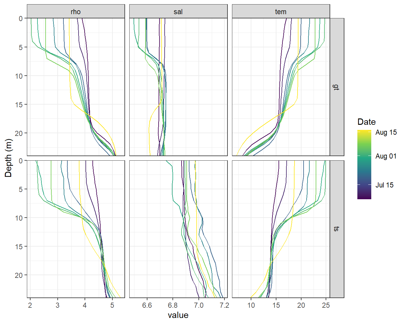
STD profiles modeled with GETM (upper panels, gt) and measured during BloomSail campaign (lower panels, ts)
ts_gt_3d <- ts_gt_3d_long %>%
  pivot_wider(values_from = "value", names_from = "source") %>%
  mutate(value_diff = gt - ts)

ts_gt_3d %>%
  ggplot(aes(value_diff, dep,
             col=date_time,
             group=date_time))+
  geom_vline(xintercept = 0, col="red")+
  geom_path()+
  scale_y_reverse(expand = c(0,0), name="Depth (m)")+
  scale_color_viridis_c(name="Date", trans = "time")+
  facet_grid(.~var, scales = "free_x")+
  labs(x="Difference GETM (gt) - Bloomsail (ts)")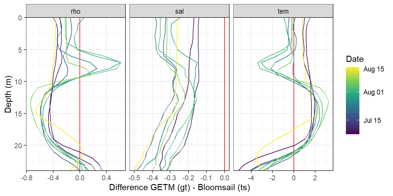
2.1.2 Heat penetration depth
As an alternative approach to the integration over the MLD or the reconstruction of CT profiles, we can estimate the mean penetration depth of the warming signal, which was defined the surface change in temperature devided by the integrated change in seawater temperature across depth.
tem_diff_surface <- ts_gt_3d_long %>%
  filter(dep < 6,
         var=="tem") %>%
  select(date_time_ID = date_time, source, tem=value) %>%
  group_by(date_time_ID, source) %>%
  summarise_all(mean, na.rm=TRUE) %>%
  ungroup()

tem_diff_surface <- tem_diff_surface %>%
  group_by(source) %>%
  arrange(date_time_ID) %>%
  mutate(tem_diff_surface = tem - lag(tem)) %>%
  ungroup() %>%
  select(-tem)

ts_gt_3d_long <- ts_gt_3d_long %>%
  filter(var=="tem") %>%
  select(date_time_ID = date_time, source, dep, tem=value) %>%
  group_by(source, dep) %>%
  arrange(date_time_ID) %>%
  mutate(tem_diff = tem - lag(tem)) %>%
  ungroup() %>%
  select(-tem)

ts_gt_3d_long <- full_join(ts_gt_3d_long, tem_diff_surface)
rm(tem_diff_surface)

tem_depth <- ts_gt_3d_long %>%
  filter(dep < 18) %>%
  group_by(date_time_ID, source) %>%
  summarise(tem_diff_int = sum(tem_diff),
            tem_diff_surface = mean(tem_diff_surface),
            tem_depth = tem_diff_int/tem_diff_surface) %>%
  ungroup()

tem_depth %>%
  ggplot(aes(date_time_ID, tem_diff_surface, col=source))+
  geom_hline(yintercept = 0)+
  geom_line()+
  geom_point()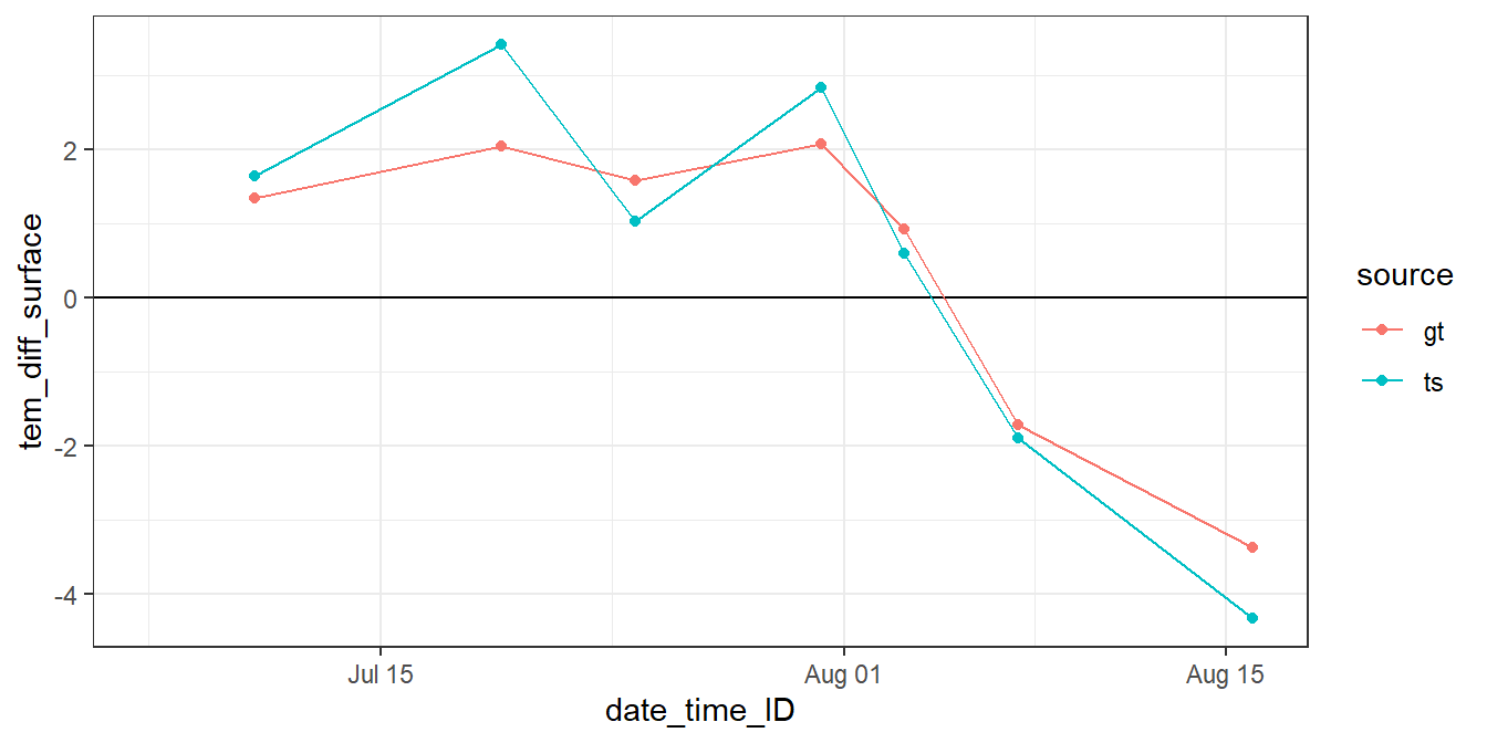
tem_depth %>%
  ggplot(aes(date_time_ID, tem_diff_int, col=source))+
  geom_hline(yintercept = 0)+
  geom_line()+
  geom_point()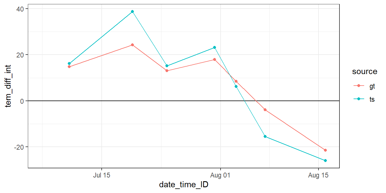
tem_depth %>%
  ggplot(aes(date_time_ID, tem_depth, col=source))+
  geom_hline(yintercept = 0)+
  geom_line()+
  geom_point()+
  scale_y_reverse()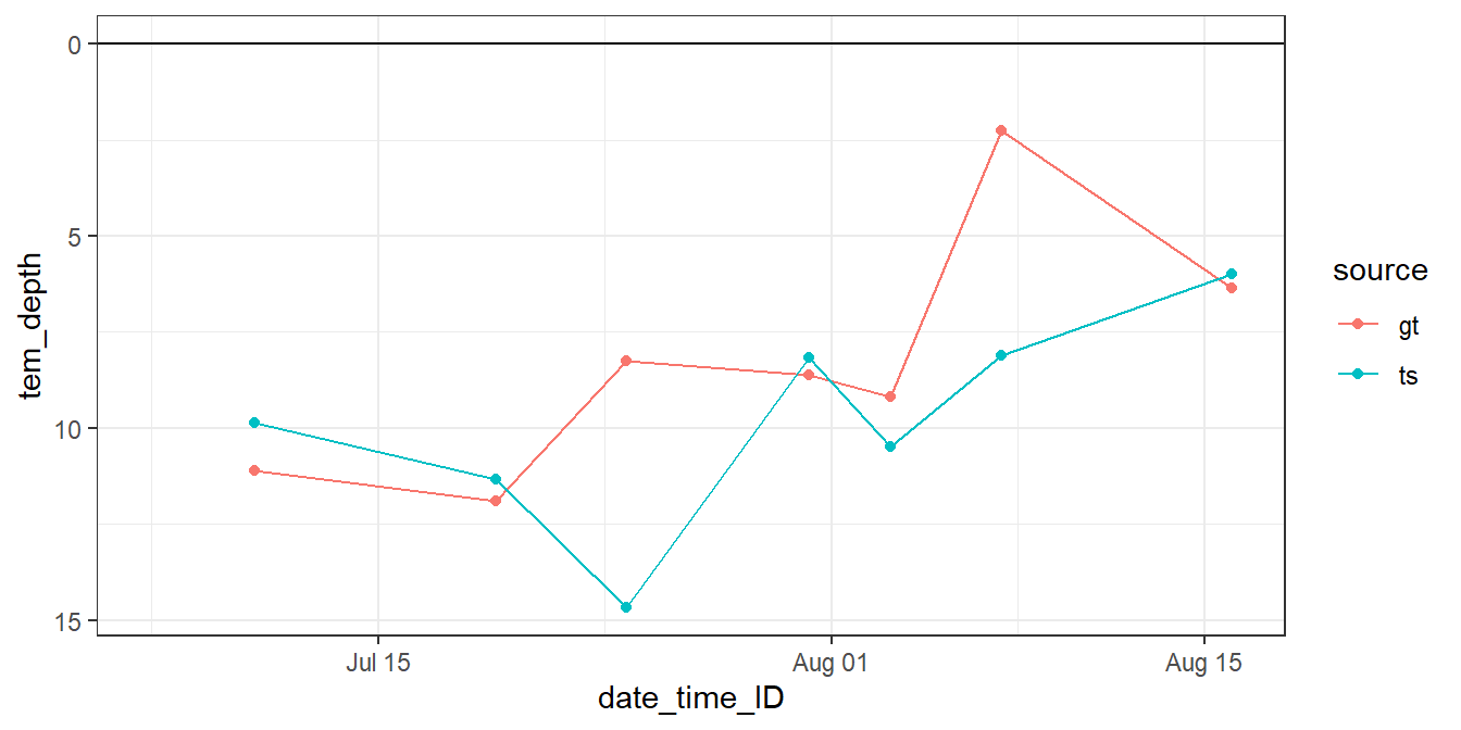
rm(ts_gt_3d, ts_gt_3d_long, ts_profiles_ID)2.2 Mixed layer depth
Mean mixed/mixing layer depth estimates based on sewater density and windspeed were extracted from 3h GETM surface data.
nc_2d <- nc_open(here("data/GETM", "Finnmaid.E.2d.2018.nc"))
#print(nc_2d)

lat <- ncvar_get(nc_2d, "latc")

time_units <- nc_2d$dim$time$units %>%     #we read the time unit from the netcdf file to calibrate the time
    substr(start = 15, stop = 33) %>%   #calculation, we take the relevant information from the string
    ymd_hms()                           # and transform it to the right format
t <- time_units + ncvar_get(nc_2d, "time") # read time vector
rm(time_units)

for (var in names(nc_2d$var)[c(3,4,6:12)]) {

#var <- "mld_rho"

array <- ncvar_get(nc_2d, var) # store the data in a 3-dimensional array
fillvalue <- ncatt_get(nc_2d, var, "_FillValue")
array[array == fillvalue$value] <- NA

array <- as.data.frame(t(array), xy=TRUE)
array <- as_tibble(array)

  gt_2d_part <- array %>%
  set_names(as.character(lat)) %>%
  mutate(date_time = t) %>%
  filter(date_time >= start_date & date_time <= end_date) %>%
  gather("lat", "value", 1:length(lat)) %>%
  mutate(lat = as.numeric(lat)) %>%
  filter(lat > low_lat, lat<high_lat) %>%
  select(-lat) %>%
  group_by(date_time) %>%
  summarise_all(list(value=~mean(.,na.rm=TRUE))) %>%
  ungroup() %>%
  mutate(var = var)

  if (exists("gt_2d")) {
    gt_2d <- bind_rows(gt_2d, gt_2d_part)
    } else {gt_2d <- gt_2d_part}

rm(array, fillvalue, gt_2d_part)

}

nc_close(nc_2d)
rm(nc_2d)

gt_2d <- gt_2d %>%
  mutate(value = round(value, 3)) %>%
  pivot_wider(values_from = value, names_from = var) %>%
  mutate(U_10 = round(sqrt(u10^2 + v10^2), 3)) %>%
  select(-c(u10, v10))


gt_2d %>%
  vroom_write((here::here("data/_summarized_data_files", file = "gt_2d.csv")))

rm(t, var, gt_2d, lat)
2.2.1 Hovmoeller Plots
gt_2d <-
  read_tsv((here::here("data/_summarized_data_files", file = "gt_2d.csv")))

gt_2d_daily <- gt_2d %>%
  mutate(day = yday(date_time)) %>%
  group_by(day) %>%
  summarise_all(list(~mean(.,na.rm=TRUE))) %>%
  ungroup() %>%
  select(-day)

p_sal <- gt_3d %>%
  ggplot()+
  geom_raster(aes(date_time, dep, fill=salt))+
  geom_vline(data=fixed_values, aes(xintercept = start))+
  geom_vline(data=fixed_values, aes(xintercept = end))+
  scale_fill_viridis_c(name="Salinity ", direction = -1)+
  scale_y_reverse()+
  coord_cartesian(expand = 0)+
  labs(y="Depth [m]")+
  theme(axis.title.x = element_blank(),
        axis.text.x = element_blank())+
  geom_line(data= gt_2d_daily,
            aes(x = date_time, y = mld_rho), color = "white")


p_tem <- gt_3d %>%
  ggplot()+
  geom_raster(aes(date_time, dep, fill=temp))+
  geom_vline(data=fixed_values, aes(xintercept = start))+
  geom_vline(data=fixed_values, aes(xintercept = end))+
  scale_fill_viridis_c(name="Temperature (°C)", option = "B")+
  scale_y_reverse()+
  coord_cartesian(expand = 0)+
  labs(y="Depth [m]", x="")+
  theme(axis.title.x = element_blank(),
        axis.text.x = element_blank())+
  geom_line(data= gt_2d_daily,
            aes(x = date_time, y = mld_rho), color = "white")

p_rho <- gt_3d %>%
  ggplot()+
  geom_raster(aes(date_time, dep, fill=rho))+
  geom_vline(data=fixed_values, aes(xintercept = start))+
  geom_vline(data=fixed_values, aes(xintercept = end))+
  scale_fill_viridis_c(name="d Rho (kg/m^3)", direction = -1)+
  scale_y_reverse()+
  coord_cartesian(expand = 0)+
  labs(y="Depth [m]", x="")+
  theme(axis.title.x = element_blank())+
  geom_line(data= gt_2d_daily,
            aes(x = date_time, y = mld_rho), color = "white")

p_age <- gt_3d %>%
  ggplot()+
  geom_raster(aes(date_time, dep, fill=SurfaceAge))+
  geom_vline(data=fixed_values, aes(xintercept = start))+
  geom_vline(data=fixed_values, aes(xintercept = end))+
  scale_fill_viridis_c(name="SurfaceAge (d)", direction = -1, trans = "sqrt")+
  scale_y_reverse()+
  coord_cartesian(expand = 0)+
  labs(y="Depth [m]", x="")+
  theme(axis.title.x = element_blank())+
  geom_line(data= gt_2d_daily,
            aes(x = date_time, y = mld_rho), color = "white")

p_sal / p_tem / p_rho / p_age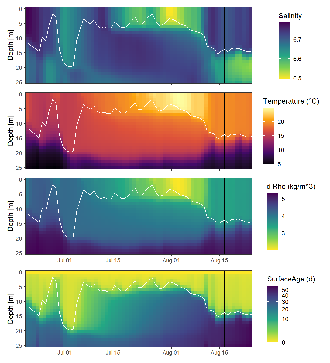
rm(p_sal, p_tem, p_rho)2.2.2 Test calculation
Mean mixed layer depth estimates were also calculated for a range of density threshold criteria, Rho lim, from sewater density based on daily mean GETM STD profiles.
gt_3d_MLD <- expand_grid(gt_3d, rho_lim = seq(0.1,0.5,0.1))

gt_3d_MLD <- gt_3d_MLD %>%
  arrange(dep) %>%
  group_by(date_time, rho_lim) %>%
  mutate(d_rho = rho - first(rho)) %>%
  filter(d_rho > rho_lim) %>%
  summarise(MLD = min(dep)) %>%
  ungroup() %>%
  mutate(rho_lim = as.factor(rho_lim))
2.2.3 Time series
gt_2d_daily_long <- gt_2d_daily %>%
  pivot_longer(4:8, names_to = "var", values_to = "value")

p_MLD_gt <- gt_2d_daily_long %>%
  ggplot()+
  geom_rect(data = fixed_values, aes(xmin=start, xmax=end, ymin=-Inf, ymax=Inf), alpha=0.2)+
  geom_hline(yintercept = 0)+
  geom_line(aes(date_time, value, col=var))+
  scale_y_reverse(limits = c(25,0))+
  scale_color_brewer(palette = "Set1", name="GETM variable")+
  labs(x="", y="MLD (m)")+
  theme(axis.title.x = element_blank())

p_MLD_recalc <- gt_3d_MLD %>%
  ggplot()+
  geom_rect(data = fixed_values, aes(xmin=start, xmax=end, ymin=-Inf, ymax=Inf), alpha=0.2)+
  geom_hline(yintercept = 0)+
  geom_line(aes(date_time, MLD, col=rho_lim))+
  scale_y_reverse(limits = c(25,0))+
  scale_color_viridis_d(name="Rho lim")+
  labs(x="", y="MLD (m)")

p_MLD_gt / p_MLD_recalc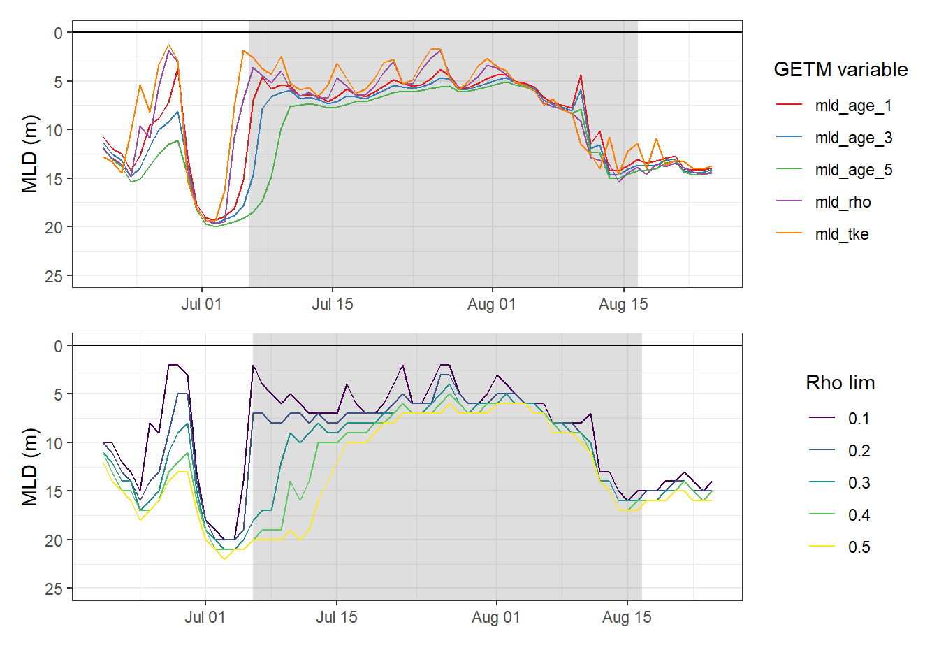
rm(p_MLD_gt, p_MLD_recalc)3 Finnmaid
3.1 Read data
Finnmaid data, including reconstructed data during LICOS operation failure.
fm <-
 read_csv(here::here("Data/_summarized_data_files",
                      "Finnmaid.csv"))

fm <- fm %>%
  filter(Area == "BS",
         date > start_date,
         date < end_date) %>%
  select(-c(Lon, Lat, patm, Teq, xCO2, route, Area)) %>%
  mutate(ID = as.factor(ID)) %>%
  rename(tem=Tem,
         sal=Sal,
         date_time = date)
3.2 CT calculation
Calculate based on fixed AT and salinity mean values.
fm <- fm %>%
  mutate(CT = carb(24,
                   var1=pCO2,
                   var2=fixed_values$AT*1e-6,
                   S=fixed_values$sal,
                   T=tem,
                   k1k2="m10", kf="dg", ks="d", gas="insitu")[,16]*1e6)
3.3 Timeseries
Calculate regional mean and sd values for each crossing of the area.
fm_ID <- fm %>%
  pivot_longer(c(pCO2, sal, tem, cO2, CT), values_to = "value", names_to = "var") %>%
  group_by(ID) %>%
  mutate(date_time_ID = mean(date_time)) %>%
  select(-date_time) %>%
  ungroup() %>%
  group_by(ID, date_time_ID, sensor, var) %>%
  summarise_all(list(~mean(.), ~sd(.), ~min(.), ~max(.)), na.rm=TRUE) %>%
  ungroup() %>%
  rename(value=mean)
Read BloomSail profile data from 1-5m to fill observational gap of Finnmaid date in second half of June.
ts_profiles_ID_long <-
  read_csv(here::here("Data/_merged_data_files", "ts_profiles_ID_long_cum.csv"))

ts_profiles_ID_long_surface <- ts_profiles_ID_long %>%
  filter(dep > 1, dep < 5) %>%
  mutate(ID = as.factor(ID)) %>%
  select(-c(sign, value_cum_sign)) %>%
  group_by(ID, date_time_ID, var) %>%
  summarise_all(list(~mean(.)), na.rm = TRUE) %>%
  ungroup()
fm_ID %>%
ggplot()+
geom_rect(data = fixed_values, aes(xmin=start, xmax=end, ymin=-Inf, ymax=Inf), alpha=0.2)+
geom_path(aes(x=date_time_ID, y=value))+
#geom_ribbon(aes(x=date_time, y=value, ymax=max, ymin=min, fill="Finnmaid"), alpha=0.3)+
geom_ribbon(aes(x=date_time_ID, y=value, ymax=value+sd, ymin=value-sd, fill="Finnmaid"), alpha=0.3)+
geom_ribbon(data = ts_profiles_ID_long_surface,
aes(x=date_time_ID, ymin=value-sd, ymax=value+sd, fill="BloomSail"), alpha=0.3)+
geom_point(aes(x=date_time_ID, y=value, col=sensor))+
geom_point(data = ts_profiles_ID_long_surface,
aes(x=date_time_ID, y=value, col="BloomSail"))+
geom_line(data = ts_profiles_ID_long_surface,
aes(x=date_time_ID, y=value, col="BloomSail"))+
facet_grid(var~., scales = "free_y")+
scale_color_brewer(palette = "Set1")+
scale_fill_brewer(palette = "Set1", name="+/- SD")
3.4 Missing observations
The observational gaps in the Finnmaid SST and CT time series were filled with two BloomSail observations. The time series was restricted to the period where BloomSail observations are available.
ts_gap <- ts_profiles_ID_long_surface %>%
  filter(ID %in% c("180718", "180723"),
         var %in% c("tem", "CT")) %>%
  select(date_time_ID, ID, var, value = value) %>%
  mutate(sensor = "BloomSail")

fm_ts_ID <- full_join(fm_ID, ts_gap) %>%
  arrange(date_time_ID) %>%
  select(-sd) %>%
  filter(var %in% c("tem", "CT")) %>%
  mutate(period = "BloomSail",
         period = if_else(date_time_ID < fixed_values$start, "pre-BloomSail", period),
         period = if_else(date_time_ID > fixed_values$end, "post-BloomSail", period))

fm_ts_ID %>%
  ggplot()+
  geom_rect(data = fixed_values,
            aes(xmin=start, xmax=end, ymin=-Inf, ymax=Inf), alpha=0.2)+
  geom_path(aes(date_time_ID, value, col=period))+
  geom_point(aes(date_time_ID, value, col=period))+
  facet_grid(var~., scales = "free_y")+
  scale_color_brewer(palette = "Set1")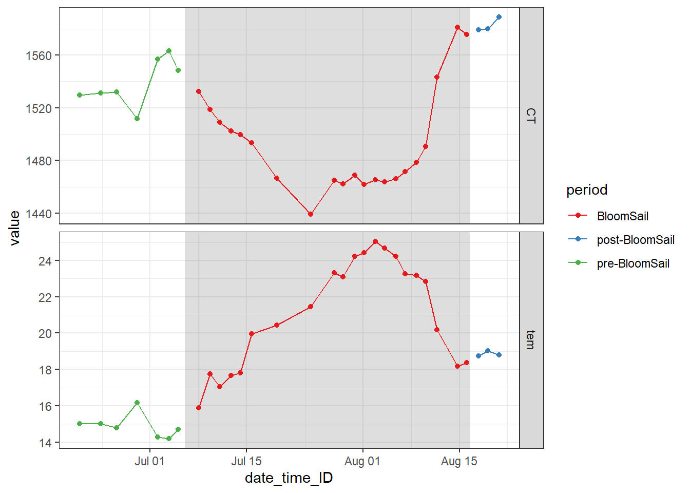
fm_ts_ID <- fm_ts_ID %>%
  filter(period == "BloomSail") %>%
  select(-period)

rm(fm_ID, fm, ts_gap, ts_profiles_ID_long_surface)
4 iCT
4.1 MLD approach
Use dCT from Finnmaid and MLD from GETM and calculate iCT as their product.
iCT_MLD <- fm_ts_ID %>%
  select(date_time_ID, var, value) %>%
  pivot_wider(values_from = value, names_from = var) %>%
  rename(SST = tem)

iCT_MLD <- full_join(iCT_MLD,
                     gt_2d_daily %>%
                       select(-c(SSS, SST, U_10)) %>%
                       rename(date_time_ID = date_time))

iCT_MLD <- iCT_MLD %>%
  pivot_longer(cols = 4:8, values_to = "MLD", names_to = "var") %>%
  arrange(date_time_ID) %>%
  group_by(var) %>%
  mutate(MLD = na.approx(MLD)) %>%
  ungroup()

iCT_MLD <- iCT_MLD %>%
  drop_na() %>%
  group_by(var) %>%
  arrange(date_time_ID) %>%
  mutate(date_time_ID_diff = as.numeric(date_time_ID - lag(date_time_ID)),
         date_time_ID_ref  = date_time_ID - (date_time_ID - lag(date_time_ID))/2,
         CT_diff = CT - lag(CT),
         SST_diff = SST - lag(SST),
         CT_i_diff = CT_diff * MLD / 1000,
         CT_i_cum = cumsum(replace_na(CT_i_diff, 0))) %>%
  ungroup()
4.1.1 Incremental and cumulative timeseries
Total incremental and cumulative CT changes inbetween cruise dates were calculated.
iCT_MLD %>%
  ggplot()+
  geom_hline(yintercept = 0)+
  geom_point(aes(date_time_ID,  0), shape=21)+
  geom_col(aes(date_time_ID_ref, CT_i_diff, fill= var),
           col="black", position = "dodge", alpha = 0.5)+
  geom_line(aes(date_time_ID,  CT_i_cum,
             col= var))+
  scale_y_continuous(breaks = seq(-100, 100, 0.2))+
  scale_fill_brewer(palette = "Set1", name="Incremental")+
  scale_color_brewer(palette = "Set1", name="Cumulative")+
  labs(y="integrated CT changes [mol/m2]", x="date")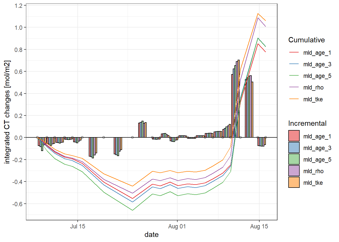
4.2 delta T appraoch
As primary production (negative changes in CT) and increase in seawater temperature have a common driver (light), the relation between both changes was investigated and will be used to reconstruct changes in CT throughout the water column.
The following analysis is restricted to the BloomSail period.
4.2.1 SST time series
fm_ts_ID %>%
  filter(var == "tem") %>%
  ggplot()+
  geom_rect(data = fixed_values, aes(xmin=start, xmax=end, ymin=-Inf, ymax=Inf), alpha=0.2)+
  geom_path(aes(x=date_time_ID, y=value, col="Finnmaid"))+
  geom_point(aes(x=date_time_ID, y=value, col="Finnmaid"))+
  geom_path(data = gt_2d, aes(x=date_time, y=SST, col="GETM 2d, 3h"))+
  geom_path(data = gt_2d_daily, aes(x=date_time, y=SST, col="GETM 2d, daily"))+
  geom_path(data = gt_3d %>% filter(dep == 3),
            aes(x=date_time, y=temp, col="GETM 3d, 3m"))+
  scale_color_brewer(palette = "Set1", name="")+
  labs(x="", y="SST (°C)")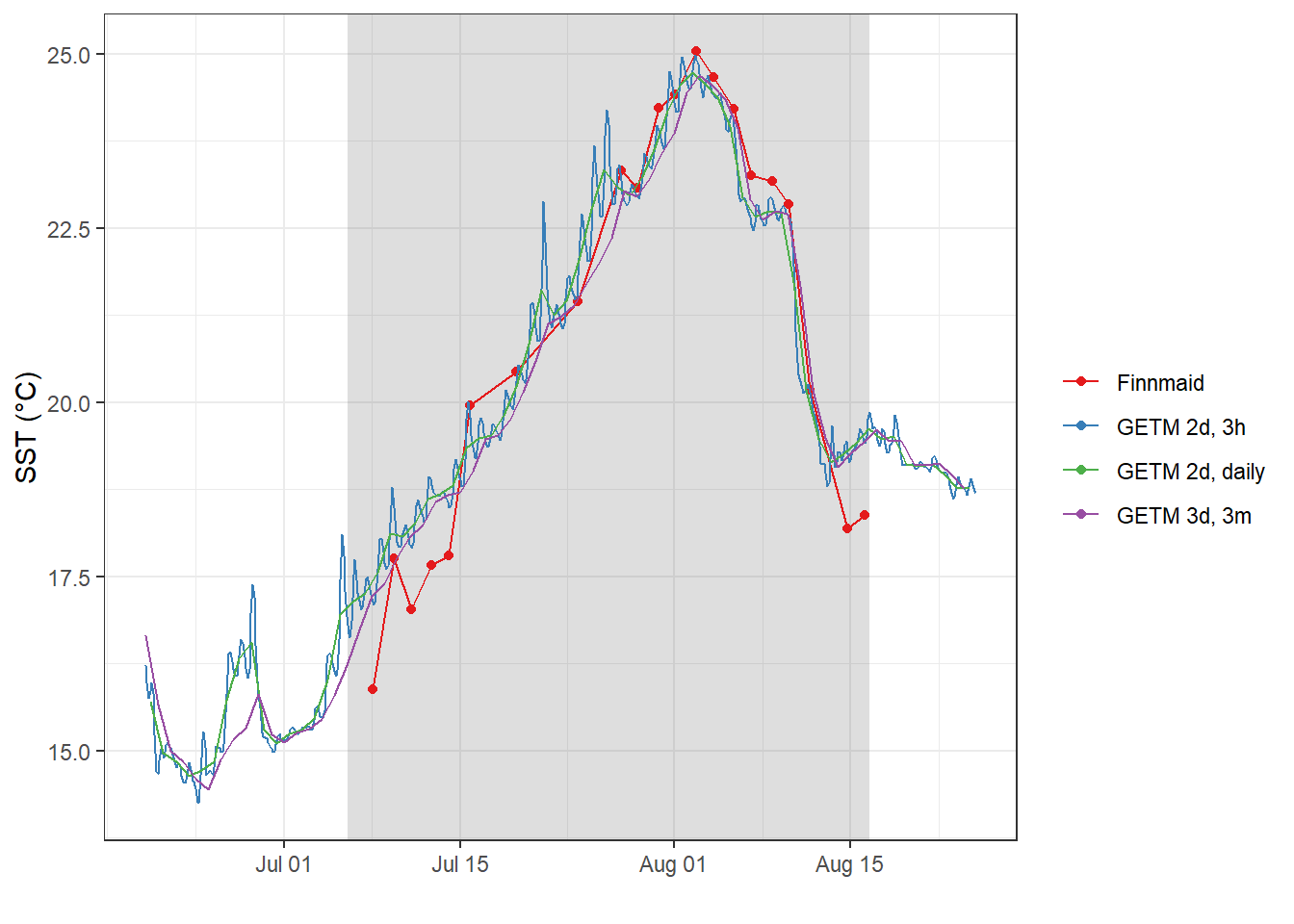
4.2.2 dCT vs dSST
To investigate the change of surface CT with SST, we merge daily mean 2d GETM and Finnmaid data. GETM observations were linearly interpolated to match the time of Finnmaid observations.
fm_ts_ID_wide <- fm_ts_ID %>%
  filter(var %in% c("CT")) %>%
  select(date_time_ID, var, value) %>%
  pivot_wider(values_from = value, names_from = var)

fm_gt_3d <- expand_grid(fm_ts_ID_wide, dep = unique(gt_3d$dep))
rm(fm_ts_ID_wide)

fm_gt_3d <- full_join(gt_3d %>% select(date_time_ID = date_time, dep, tem = temp),
                      fm_gt_3d)
fm_gt_3d <- fm_gt_3d %>%
arrange(date_time_ID) %>%
group_by(dep) %>%
mutate(tem = approxfun(date_time_ID, tem)(date_time_ID)) %>%
ungroup() %>%
arrange(dep) %>%
filter(!is.na(CT))CT_tem <- CT_tem %>%
arrange(date_time_ID) %>%
mutate(CT = na.approx(CT, na.rm = FALSE),
FM = na.approx(FM, na.rm = FALSE)) %>%
drop_na()
rolling_mean <- rollify(~mean(.x, na.rm = TRUE), window = 3)
CT_tem <- CT_tem %>%
mutate(CT_rm = rolling_mean(CT) %>% lead(n = 1),
FM_rm = rolling_mean(FM) %>% lead(n = 1),
gt_rm = rolling_mean(gt) %>% lead(n = 1))p_SST <- CT_tem %>%
ggplot()+
geom_rect(data = fixed_values, aes(xmin=start, xmax=end, ymin=-Inf, ymax=Inf), alpha=0.2)+
geom_point(aes(date_time_ID, FM, col="FM"))+
geom_path(aes(date_time_ID, FM_rm, col="FM"))+
geom_point(aes(date_time_ID, gt, col="gt"))+
geom_path(aes(date_time_ID, gt_rm, col="gt"))+
scale_color_brewer(palette = "Set1", name="")+
theme(axis.title.x = element_blank(),
axis.text.x = element_blank())
p_CT <- CT_tem %>%
ggplot()+
geom_rect(data = fixed_values, aes(xmin=start, xmax=end, ymin=-Inf, ymax=Inf), alpha=0.2)+
geom_point(aes(date_time_ID, CT, col="FM"))+
geom_path(aes(date_time_ID, CT_rm, col="FM"))+
scale_color_brewer(palette = "Set1", name="")+
theme(axis.title.x = element_blank())
p_SST / p_CT
CT_tem <- CT_tem %>%
select(-c(CT, FM, gt)) %>%
rename(CT = CT_rm,
FM = FM_rm,
gt = gt_rm)CT_tem <- fm_gt_3d %>%
filter(dep == 3) %>%
arrange(date_time_ID) %>%
mutate(CT_diff = CT - lag(CT),
SST_diff = tem - lag(tem)) %>%
select(-tem)
CT_tem %>%
ggplot()+
geom_hline(yintercept = 0)+
geom_vline(xintercept = 0)+
geom_smooth(aes(SST_diff, CT_diff), method = "lm", se=FALSE)+
geom_point(aes(SST_diff, CT_diff, fill=date_time_ID), shape=21)+
scale_fill_viridis_c(trans = "time", name="Date")
CT_tem <- CT_tem %>%
  mutate(factor = CT_diff/SST_diff,
         factor = if_else(is.na(factor), 0, factor))
Time series of incremental changes in CT and SST help to identify measurement days during which changes in both parameters deviate from the expected correlation (factor).
CT_tem_long <- CT_tem %>%
  pivot_longer(c(CT_diff, SST_diff, factor), values_to = "value", names_to = "var")#

CT_tem_long %>%
  ggplot(aes(date_time_ID, value))+
  geom_hline(yintercept = 0)+
  geom_point()+
  geom_line()+
  scale_color_brewer(palette = "Set1")+
  facet_grid(var~., scales = "free_y")+
  theme(axis.title.x = element_blank())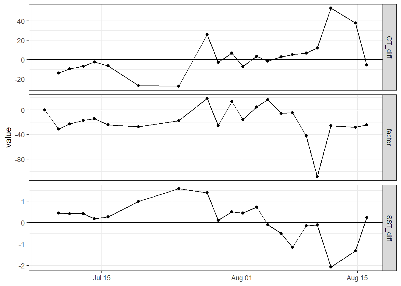
The ratio of surface changes in CT with SST based on GETM SST was used.
CT_tem <- expand_grid(CT_tem %>% select(date_time_ID, factor),
                      dep = unique(fm_gt_3d$dep))

fm_gt_3d <- full_join(fm_gt_3d %>% select(date_time_ID, dep, tem),
                      CT_tem %>%  select(date_time_ID, dep, factor))
fm_gt_3d <- fm_gt_3d %>%
group_by(dep) %>%
arrange(date_time_ID) %>%
mutate(tem_diff = tem - lag(tem)) %>%
ungroup() %>%
mutate(CT_diff = tem_diff * factor) %>%
select(-factor)The reconstructed incremental changes are added up to derive cummulative CT changes throughout the water column.
fm_gt_3d <- fm_gt_3d %>%
  group_by(dep) %>%
  arrange(date_time_ID) %>%
  mutate(date_time_ID_diff = as.numeric(date_time_ID - lag(date_time_ID)),
         date_time_ID_ref  = date_time_ID - (date_time_ID - lag(date_time_ID))/2,
         CT_diff_daily = CT_diff / date_time_ID_diff,
         CT_cum = cumsum(replace_na(CT_diff, 0))) %>%
  ungroup()
4.2.3 Profiles of incremental changes
Changes of seawater parameters at each depth were reconstructed from one cruise day to the next and divided by the number of days inbetween.
fm_gt_3d %>%
  arrange(dep) %>%
  ggplot(aes(CT_diff_daily, dep, col=date_time_ID, group=date_time_ID))+
  geom_vline(xintercept = 0)+
  geom_point()+
  geom_path()+
  scale_y_reverse()+
  scale_color_viridis_c(trans = "time")+
  labs(x="Change of CT inbetween cruises per day")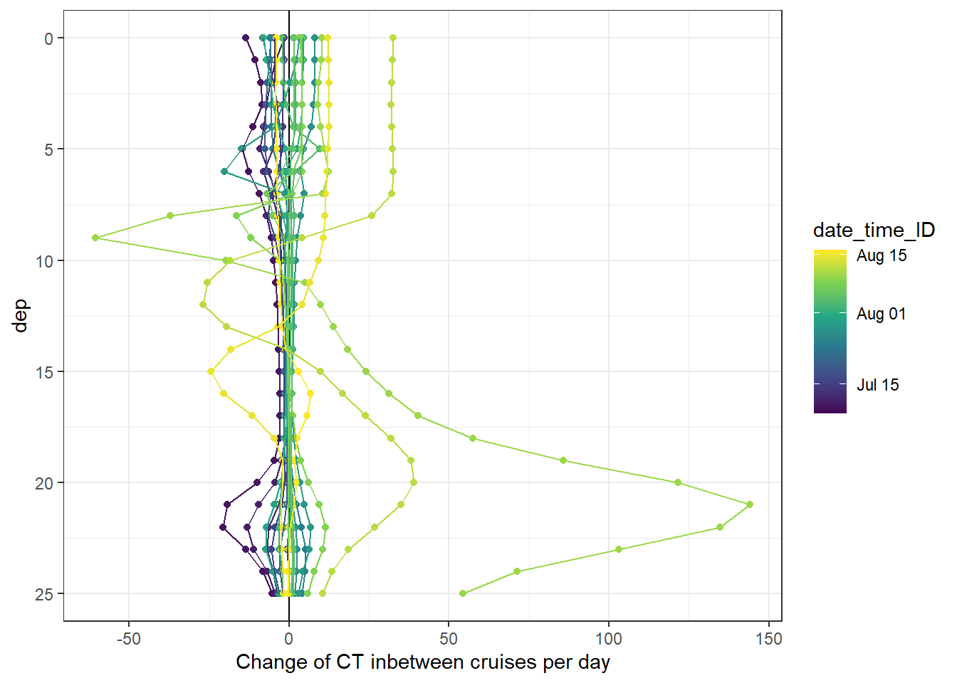
fm_gt_3d %>%
  arrange(dep) %>%
  ggplot(aes(tem_diff, dep, col=date_time_ID, group=date_time_ID))+
  geom_vline(xintercept = 0)+
  geom_point()+
  geom_path()+
  scale_y_reverse()+
  scale_color_viridis_c(trans = "time")+
  labs(x="Change of temperature inbetween cruises per day")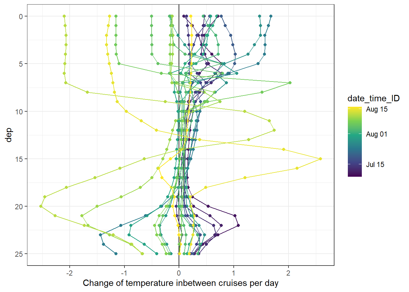
4.2.4 Profiles of cumulative changes
Cumulative changes of seawater parameters were calculated at each depth relative to the first cruise day on July 5.
fm_gt_3d %>%
  arrange(dep) %>%
  ggplot(aes(CT_cum, dep, col=date_time_ID, group=date_time_ID))+
  geom_vline(xintercept = 0)+
  geom_point()+
  geom_path()+
  scale_y_reverse()+
  scale_color_viridis_c(trans = "time")+
  labs(x="Cumulative change of CT")
4.2.5 Hovmoeller daily changes
Hoevmoeller plots were generated for the reconstructed daily and cumulative changes in CT. Absolute values are not reproducible with this approach.
bin_tem <- 0.25

fm_gt_3d %>%
  filter(dep < 26) %>%
  ggplot()+
  geom_contour_fill(aes(x=date_time_ID_ref, y=dep, z=tem_diff),
                    breaks = MakeBreaks(bin_tem),
                    col="black")+
  geom_point(aes(x=date_time_ID, y=c(25)), size=3, shape=24, fill="white")+
  scale_fill_divergent(breaks = MakeBreaks(bin_tem),
                       guide = "colorstrip",
                       name="Tem (°C)")+
  scale_y_reverse()+
  theme_bw()+
  labs(y="Depth (m)")+
  coord_cartesian(expand = 0)+
  theme(axis.title.x = element_blank(),
        axis.text.x = element_blank())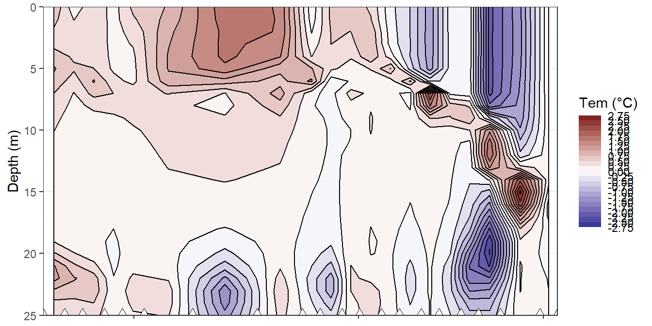
Hovmoeller plots of modelled daily changes in temperature.
rm(bin_tem)bin_CT <- 10
fm_gt_3d %>%
filter(dep < 15) %>%
ggplot()+
geom_contour_fill(aes(x=date_time_ID_ref, y=dep, z=CT_diff_daily),
breaks = MakeBreaks(bin_CT),
col="black")+
geom_point(aes(x=date_time_ID, y=c(14)), size=3, shape=24, fill="white")+
scale_fill_divergent(breaks = MakeBreaks(bin_CT),
guide = "colorstrip",
name="CT (µmol/kg)")+
scale_y_reverse()+
theme_bw()+
labs(y="Depth (m)")+
coord_cartesian(expand = 0)+
theme(axis.title.x = element_blank(),
axis.text.x = element_blank())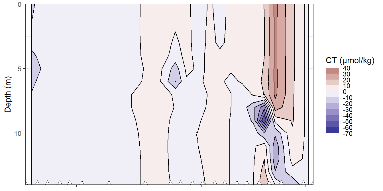
Hovmoeller plots of daily reconstructed changes in CT.
rm(bin_CT)4.2.6 Hovmoeller cumulative changes
bin_CT <- 30

fm_gt_3d %>%
  filter(dep < 15) %>%
  ggplot()+
  geom_contour_fill(aes(x=date_time_ID, y=dep, z=CT_cum),
                    breaks = MakeBreaks(bin_CT),
                    col="black")+
  geom_point(aes(x=date_time_ID, y=c(14)), size=3, shape=24, fill="white")+
  scale_fill_divergent(breaks = MakeBreaks(bin_CT),
                       guide = "colorstrip",
                       name="CT (µmol/kg)")+
  scale_y_reverse()+
  theme_bw()+
  labs(y="Depth (m)")+
  coord_cartesian(expand = 0)+
  theme(axis.title.x = element_blank(),
        axis.text.x = element_blank())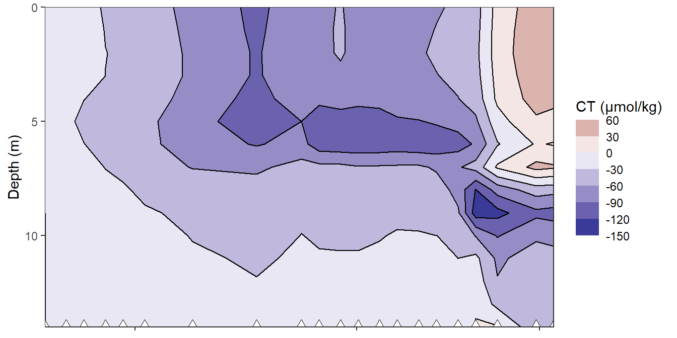
Hovmoeller plots of cumulative reconstructed changes in CT.
rm(bin_CT)4.2.7 Heat penetration depth
As an alternative approach to the integration over the MLD or the reconstruction of CT profiles, we can estimate the mean penetration depth of the warming signal, which was defined the surface change in temperature devided by the integrated change in seawater temperature across depth.
tem_diff_surface <- fm_gt_3d %>%
  filter(dep < 6) %>%
  select(date_time_ID, tem_diff_surface=tem_diff) %>%
  group_by(date_time_ID) %>%
  summarise_all(mean, na.rm=TRUE) %>%
  ungroup()

fm_gt_3d <- full_join(fm_gt_3d, tem_diff_surface)
rm(tem_diff_surface)

tem_depth <- fm_gt_3d %>%
  filter(dep < 18) %>%
  group_by(date_time_ID) %>%
  summarise(tem_diff_int = sum(tem_diff),
            tem_diff_surface = mean(tem_diff_surface),
            tem_depth = tem_diff_int/tem_diff_surface) %>%
  ungroup()

tem_depth %>%
  ggplot(aes(date_time_ID, tem_depth))+
  geom_hline(yintercept = 0)+
  geom_line()+
  geom_point()+
  scale_y_reverse()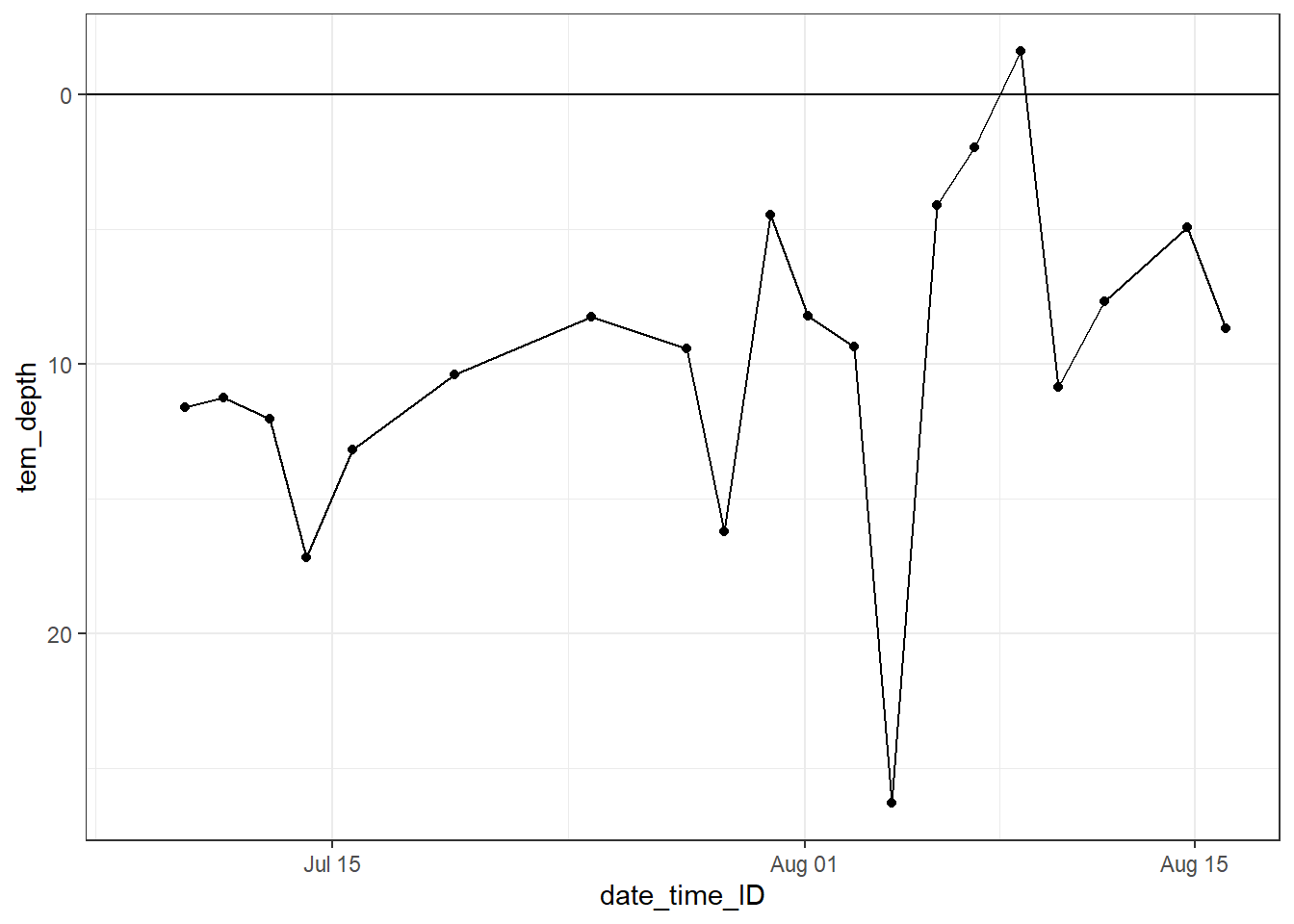
4.3 iCT time series
Total incremental and cumulative CT changes inbetween cruise dates were calculated for the upper 10 m of the water body.
iCT_dT <- fm_gt_3d %>%
  filter(dep < 10) %>%
  group_by(date_time_ID, date_time_ID_ref) %>%
  summarise(CT_i_diff = sum(CT_diff)/1000,
            CT_i_cum = sum(CT_cum)/1000) %>%
  ungroup()


iCT_dT %>%
  ggplot()+
  geom_hline(yintercept = 0)+
  geom_point(aes(date_time_ID,  0), shape=21)+
  geom_col(aes(date_time_ID_ref, CT_i_diff),
           position = "dodge", alpha=0.3)+
  geom_line(aes(date_time_ID, CT_i_cum))+
  scale_color_viridis_d(name="Depth limit (m)")+
  scale_fill_viridis_d(name="Depth limit (m)")+
  labs(y="iCT [mol/m2]", x="")+
  theme_bw()
5 GETM Windspeed
gt_2d %>%
  ggplot()+
  geom_rect(data = fixed_values, aes(xmin=start, xmax=end, ymin=-Inf, ymax=Inf), alpha=0.2)+
  geom_line(aes(x= date_time, y = U_10, col="3-hourly"))+
  geom_line(data = gt_2d_daily,
            aes(x= date_time, y = U_10, col="Daily mean"))+
  labs(y="U (m/s)", x = "Date")+
  scale_color_brewer(palette = "Set1", name="", direction = -1)+
  theme_bw()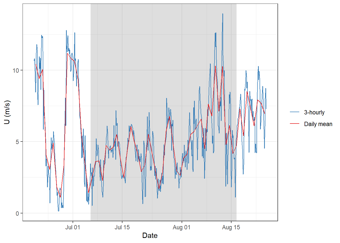
6 Open tasks / questions
- Can delta T approach be improved by:
- Using a mean CT/SST factor -> not meaningful, because it assumes steady relation between dCT and dT
- Using the cumulative values at iCT min
- Plot cumulative changes in GETM temperature: Profile + Hovmoeller
sessionInfo()R version 3.6.3 (2020-02-29)
Platform: i386-w64-mingw32/i386 (32-bit)
Running under: Windows 10 x64 (build 18363)
Matrix products: default
locale:
[1] LC_COLLATE=English_Germany.1252 LC_CTYPE=English_Germany.1252
[3] LC_MONETARY=English_Germany.1252 LC_NUMERIC=C
[5] LC_TIME=English_Germany.1252
attached base packages:
[1] stats graphics grDevices utils datasets methods base
other attached packages:
[1] metR_0.6.0 zoo_1.8-7 patchwork_1.0.0 seacarb_3.2.13
[5] oce_1.2-0 gsw_1.0-5 testthat_2.3.2 here_0.1
[9] lubridate_1.7.4 vroom_1.2.0 ncdf4_1.17 forcats_0.5.0
[13] stringr_1.4.0 dplyr_0.8.5 purrr_0.3.3 readr_1.3.1
[17] tidyr_1.0.2 tibble_3.0.0 ggplot2_3.3.0 tidyverse_1.3.0
[21] workflowr_1.6.1
loaded via a namespace (and not attached):
[1] Rcpp_1.0.4 whisker_0.4 knitr_1.28 xml2_1.3.0
[5] magrittr_1.5 splines_3.6.3 hms_0.5.3 rvest_0.3.5
[9] tidyselect_1.0.0 bit_1.1-15.2 viridisLite_0.3.0 colorspace_1.4-1
[13] lattice_0.20-41 R6_2.4.1 rlang_0.4.5 fansi_0.4.1
[17] broom_0.5.5 xfun_0.12 dbplyr_1.4.2 modelr_0.1.6
[21] withr_2.1.2 git2r_0.26.1 ellipsis_0.3.0 htmltools_0.4.0
[25] assertthat_0.2.1 bit64_0.9-7 rprojroot_1.3-2 digest_0.6.25
[29] lifecycle_0.2.0 Matrix_1.2-18 haven_2.2.0 rmarkdown_2.1
[33] sp_1.4-1 compiler_3.6.3 cellranger_1.1.0 pillar_1.4.3
[37] scales_1.1.0 backports_1.1.5 generics_0.0.2 jsonlite_1.6.1
[41] httpuv_1.5.2 pkgconfig_2.0.3 rstudioapi_0.11 munsell_0.5.0
[45] plyr_1.8.6 highr_0.8 httr_1.4.1 tools_3.6.3
[49] grid_3.6.3 nlme_3.1-145 data.table_1.12.8 gtable_0.3.0
[53] checkmate_2.0.0 mgcv_1.8-31 DBI_1.1.0 cli_2.0.2
[57] readxl_1.3.1 yaml_2.2.1 crayon_1.3.4 RColorBrewer_1.1-2
[61] farver_2.0.3 later_1.0.0 promises_1.1.0 fs_1.4.0
[65] vctrs_0.2.4 memoise_1.1.0 glue_1.3.2 evaluate_0.14
[69] labeling_0.3 reprex_0.3.0 stringi_1.4.6