Reconstruction of NCP based on surface pCO2 and CTD data
Jens Daniel Müller
20 March, 2020
Last updated: 2020-03-20
Checks: 7 0
Knit directory: BloomSail/
This reproducible R Markdown analysis was created with workflowr (version 1.6.0). The Checks tab describes the reproducibility checks that were applied when the results were created. The Past versions tab lists the development history.
Great! Since the R Markdown file has been committed to the Git repository, you know the exact version of the code that produced these results.
Great job! The global environment was empty. Objects defined in the global environment can affect the analysis in your R Markdown file in unknown ways. For reproduciblity it’s best to always run the code in an empty environment.
The command set.seed(20191021) was run prior to running the code in the R Markdown file. Setting a seed ensures that any results that rely on randomness, e.g. subsampling or permutations, are reproducible.
Great job! Recording the operating system, R version, and package versions is critical for reproducibility.
Nice! There were no cached chunks for this analysis, so you can be confident that you successfully produced the results during this run.
Great job! Using relative paths to the files within your workflowr project makes it easier to run your code on other machines.
Great! You are using Git for version control. Tracking code development and connecting the code version to the results is critical for reproducibility. The version displayed above was the version of the Git repository at the time these results were generated.
Note that you need to be careful to ensure that all relevant files for the analysis have been committed to Git prior to generating the results (you can use wflow_publish or wflow_git_commit). workflowr only checks the R Markdown file, but you know if there are other scripts or data files that it depends on. Below is the status of the Git repository when the results were generated:
Ignored files:
    Ignored:    .Rhistory
    Ignored:    .Rproj.user/
    Ignored:    data/Finnmaid_2018/
    Ignored:    data/Maps/
    Ignored:    data/Ostergarnsholm/
    Ignored:    data/TinaV/
    Ignored:    data/_merged_data_files/
    Ignored:    data/_summarized_data_files/

Unstaged changes:
    Deleted:    analysis/BloomSail_surface.Rmd
    Deleted:    analysis/MLD.Rmd
    Deleted:    analysis/data_base.Rmd
    Deleted:    analysis/gas_exchange.Rmd
Note that any generated files, e.g. HTML, png, CSS, etc., are not included in this status report because it is ok for generated content to have uncommitted changes.
There are no past versions. Publish this analysis with wflow_publish() to start tracking its development.
library(tidyverse)
library(seacarb)
library(patchwork)
library(metR)
1 Sensor data
1m gridded, downcast profiles were used. CO2-data at depths other than 3-4m were discarded to simulate a situation were only surface CO2 observations are available.
df <-
  read_csv(here::here("Data/_merged_data_files", "BloomSail_CTD_HydroC_CT_cumulative_profiles.csv"))

df <- df %>%
  select(1:5) %>%
  pivot_wider(names_from = "parameter", values_from = "value") %>%
  mutate(ID = as.factor(ID),
         CT = if_else(dep==3.5, CT, NaN))
2 CT vs temperature
As primary production (negative changes in CT) and increase in seawater temperature have a common driver (light), the relation between both changes was investigated.
df_CT <- df %>%
  drop_na() %>%
  arrange(date_time_ID) %>%
  mutate(dCT = CT - lag(CT, default = first(CT)))

df <- df %>%
  group_by(dep) %>%
  arrange(date_time_ID) %>%
  mutate(dtem = tem - lag(tem, default = first(tem))) %>%
  ungroup()

df <- full_join(df, df_CT)
rm(df_CT)

df %>%
  filter(!is.na(dCT), dCT != 0) %>%
  ggplot(aes(dtem, dCT))+
  geom_hline(yintercept = 0)+
  geom_vline(xintercept = 0)+
  geom_path()+
  geom_point(aes(fill=as.factor(ID)), shape=21)+
  scale_fill_viridis_d()
df_factor <- df %>%
  drop_na() %>%
  mutate(factor = dCT/dtem,
         factor = if_else(is.na(factor), 0, factor)) %>%
  select(ID, factor)

df <- full_join(df, df_factor)
rm(df_factor)

df <- df %>%
  group_by(ID) %>%
  mutate(diff_value = dtem * factor) %>%
  ungroup() %>%
  select(-factor)
df <- df %>%
group_by(dep) %>%
arrange(date_time_ID) %>%
mutate(diff_time = as.numeric(date_time_ID - lag(date_time_ID)),
diff_value_daily = diff_value / diff_time,
cum_value = cumsum(diff_value))2.1 Profiles of incremental changes
Changes of seawater parameters at each depth are calculated from one cruise day to the next and divided by the number of days inbetween.
df %>%
  arrange(dep) %>%
  ggplot(aes(diff_value_daily, dep, col=ID))+
  geom_vline(xintercept = 0)+
  geom_point()+
  geom_path()+
  scale_y_reverse()+
  scale_color_viridis_d()+
  #facet_wrap(~parameter, scales = "free_x")+
  labs(x="Change of value inbetween cruises per day")
2.2 Profiles of cumulative changes
Cumulative changes of seawater parameters were calculated at each depth relative to the first cruise day on July 5.
df %>%
  arrange(dep) %>%
  ggplot(aes(cum_value, dep, col=ID))+
  geom_vline(xintercept = 0)+
  geom_point()+
  geom_path()+
  scale_y_reverse()+
  scale_color_viridis_d()+
  labs(x="Cumulative change of value")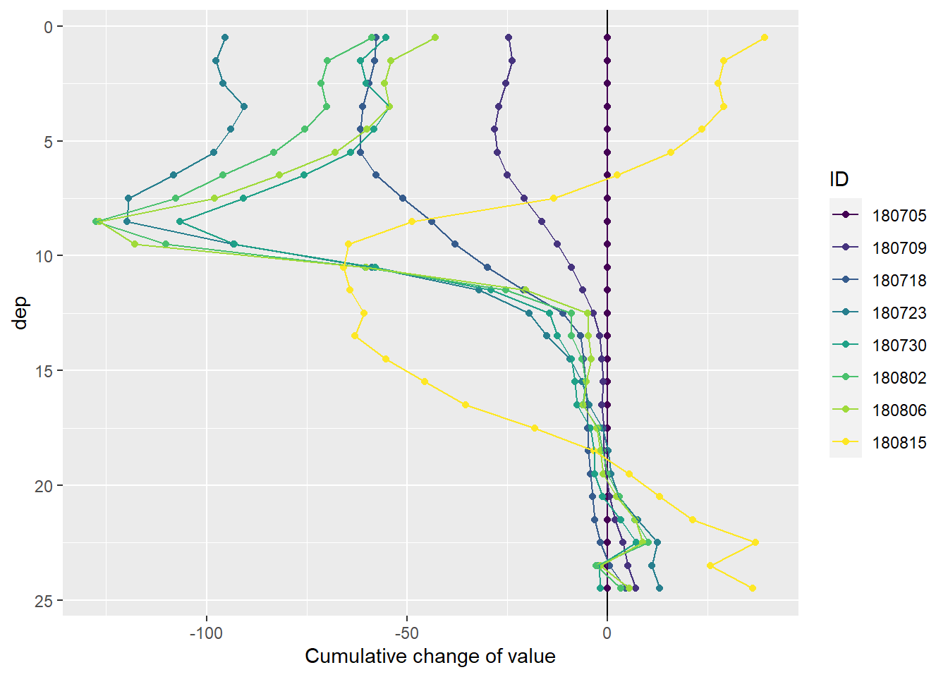
Cumulative positive and negative changes of seawater parameters were calculated separately at each depth relative to the first cruise day on July 5.
df <- df %>%
  mutate(sign = if_else(diff_value < 0, "neg", "pos")) %>%
  group_by(dep, sign) %>%
  arrange(date_time_ID) %>%
  mutate(cum_value_sign = cumsum(diff_value)) %>%
  ungroup()

df %>%
  arrange(dep) %>%
  ggplot(aes(cum_value_sign, dep, col=ID))+
  geom_vline(xintercept = 0)+
  geom_point()+
  geom_path()+
  scale_y_reverse()+
  scale_color_viridis_d()+
  scale_fill_viridis_d()+
  facet_wrap(~sign, scales = "free_x", ncol=4)+
  labs(x="Cumulative directional change of value")
3 Timeseries
3.1 Incremental and cumulative
Total incremental and cumulative CT changes inbetween cruise dates were calculated for 5m depth intervals.
NCP <- df %>%
  mutate(dep = cut(dep, seq(0,30,5))) %>%
  group_by(ID, date_time_ID, dep, sign) %>%
  summarise(dCT = sum(diff_value)/1000) %>%
  ungroup()

NCP <- NCP %>%
  group_by(sign, dep) %>%
  arrange(date_time_ID) %>%
  mutate(dCT_cum = cumsum(dCT)) %>%
  ungroup()

NCP_grid <- expand_grid(
  unique(NCP$date_time_ID),
  unique(NCP$dep),
  unique(NCP$sign)
)

NCP_grid <- NCP_grid %>%
  set_names(c("date_time_ID","dep", "sign"))

NCP <- full_join(NCP, NCP_grid)

rm(NCP_grid)

NCP <- NCP %>%
  arrange(sign, dep, date_time_ID) %>%
  group_by(sign, dep) %>%
  fill(dCT_cum) %>%
  ungroup() %>%
  mutate(dCT_cum = if_else(is.na(dCT_cum), 0, dCT_cum))
p_iNCP <- NCP %>%
ggplot(aes(date_time_ID, dCT, fill=dep))+
geom_hline(yintercept = 0)+
geom_bar(stat="identity", col="black")+
scale_fill_viridis_d()+
scale_y_continuous(breaks = seq(-100, 100, 0.2))+
facet_grid(rev(sign)~., scales = "free_y", space = "free_y")+
theme(strip.background = element_blank(),
strip.text = element_blank())+
labs(y="integrated, directional CT changes [mol/m2]", x="date")
p_iNCPcum <- NCP %>%
ggplot(aes(date_time_ID, dCT_cum, fill=dep))+
geom_hline(yintercept = 0)+
geom_area(col="black")+
scale_fill_viridis_d()+
scale_y_continuous(breaks = seq(-100, 100, 0.2))+
facet_grid(rev(sign)~., scales = "free_y", space = "free_y")+
theme(strip.background = element_blank(),
strip.text = element_blank())+
labs(y="integrated, cumulative, directional CT changes [mol/m2]", x="date")
(p_iNCP / p_iNCPcum)+
plot_layout(guides = 'collect')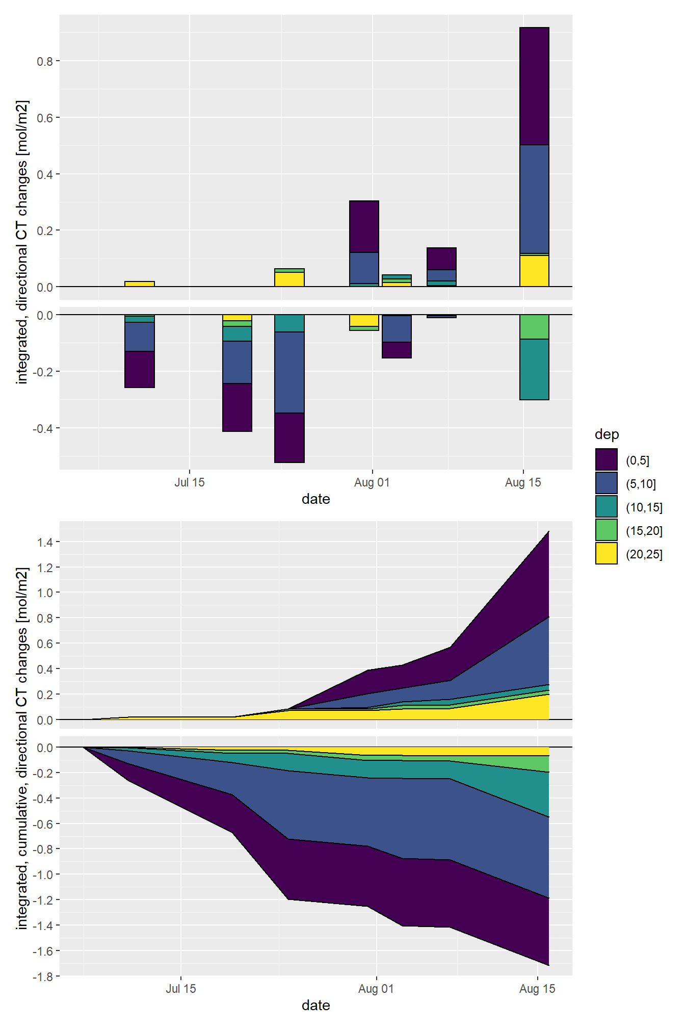
rm(p_iNCP, p_iNCPcum)4 Hovmoeller plots
4.1 Daily changes
bin_CT <- 2.5

df %>%
  ggplot()+
  geom_contour_fill(aes(x=date_time_ID, y=dep, z=diff_value_daily),
                    breaks = MakeBreaks(bin_CT),
                    col="black")+
  geom_point(aes(x=date_time_ID, y=c(24.5)), size=3, shape=24, fill="white")+
  scale_fill_divergent(breaks = MakeBreaks(bin_CT),
                       guide = "colorstrip",
                       name="CT (µmol/kg)")+
  scale_y_reverse()+
  theme_bw()+
  labs(y="Depth (m)")+
  coord_cartesian(expand = 0)+
  theme(axis.title.x = element_blank(),
        axis.text.x = element_blank())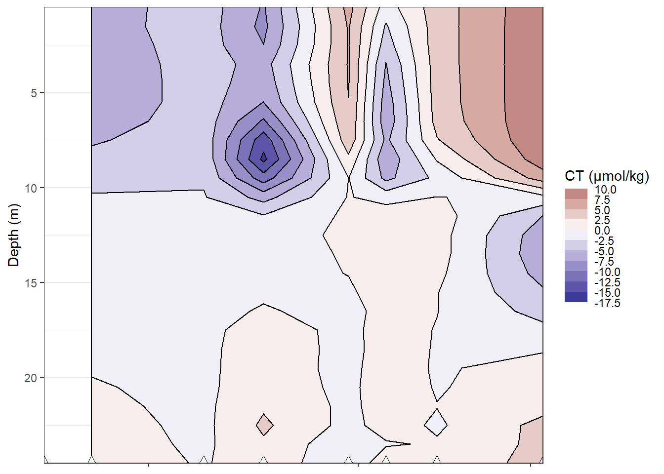
Hovmoeller plots of daily changes in CT and temperature. Note: Daily changes are currently plotted against the day when they were observed compared to the previous transect, although plotting against the mean date would be more plausible.
sessionInfo()R version 3.5.0 (2018-04-23)
Platform: x86_64-w64-mingw32/x64 (64-bit)
Running under: Windows 10 x64 (build 18363)
Matrix products: default
locale:
[1] LC_COLLATE=English_United States.1252
[2] LC_CTYPE=English_United States.1252
[3] LC_MONETARY=English_United States.1252
[4] LC_NUMERIC=C
[5] LC_TIME=English_United States.1252
attached base packages:
[1] stats graphics grDevices utils datasets methods base
other attached packages:
[1] metR_0.5.0 patchwork_1.0.0 seacarb_3.2.12 oce_1.2-0
[5] gsw_1.0-5 testthat_2.3.1 forcats_0.4.0 stringr_1.4.0
[9] dplyr_0.8.3 purrr_0.3.3 readr_1.3.1 tidyr_1.0.0
[13] tibble_2.1.3 ggplot2_3.3.0 tidyverse_1.3.0
loaded via a namespace (and not attached):
[1] nlme_3.1-137 bitops_1.0-6 fs_1.3.1
[4] lubridate_1.7.4 httr_1.4.1 rprojroot_1.3-2
[7] tools_3.5.0 backports_1.1.5 R6_2.4.0
[10] DBI_1.0.0 colorspace_1.4-1 withr_2.1.2
[13] sp_1.3-2 tidyselect_0.2.5 gridExtra_2.3
[16] compiler_3.5.0 git2r_0.26.1 cli_1.1.0
[19] rvest_0.3.5 xml2_1.2.2 labeling_0.3
[22] scales_1.0.0 checkmate_1.9.4 digest_0.6.22
[25] foreign_0.8-70 rmarkdown_2.0 pkgconfig_2.0.3
[28] htmltools_0.4.0 dbplyr_1.4.2 highr_0.8
[31] maps_3.3.0 rlang_0.4.5 readxl_1.3.1
[34] rstudioapi_0.10 generics_0.0.2 jsonlite_1.6
[37] RCurl_1.95-4.12 magrittr_1.5 Formula_1.2-3
[40] dotCall64_1.0-0 Matrix_1.2-14 Rcpp_1.0.2
[43] munsell_0.5.0 lifecycle_0.1.0 stringi_1.4.3
[46] yaml_2.2.0 plyr_1.8.4 grid_3.5.0
[49] maptools_0.9-8 formula.tools_1.7.1 promises_1.1.0
[52] crayon_1.3.4 lattice_0.20-35 haven_2.2.0
[55] hms_0.5.2 zeallot_0.1.0 knitr_1.26
[58] pillar_1.4.2 reprex_0.3.0 glue_1.3.1
[61] evaluate_0.14 data.table_1.12.6 modelr_0.1.5
[64] operator.tools_1.6.3 vctrs_0.2.0 spam_2.3-0.2
[67] httpuv_1.5.2 cellranger_1.1.0 gtable_0.3.0
[70] assertthat_0.2.1 xfun_0.10 broom_0.5.3
[73] later_1.0.0 viridisLite_0.3.0 memoise_1.1.0
[76] fields_9.9 workflowr_1.6.0 ellipsis_0.3.0
[79] here_0.1