Response time correction of Contros HydroC pCO2 data
Jens Daniel Müller
09 December, 2019
Last updated: 2019-12-09
Checks: 7 0
Knit directory: BloomSail/
This reproducible R Markdown analysis was created with workflowr (version 1.5.0). The Checks tab describes the reproducibility checks that were applied when the results were created. The Past versions tab lists the development history.
Great! Since the R Markdown file has been committed to the Git repository, you know the exact version of the code that produced these results.
Great job! The global environment was empty. Objects defined in the global environment can affect the analysis in your R Markdown file in unknown ways. For reproduciblity it’s best to always run the code in an empty environment.
The command set.seed(20191021) was run prior to running the code in the R Markdown file. Setting a seed ensures that any results that rely on randomness, e.g. subsampling or permutations, are reproducible.
Great job! Recording the operating system, R version, and package versions is critical for reproducibility.
Nice! There were no cached chunks for this analysis, so you can be confident that you successfully produced the results during this run.
Great job! Using relative paths to the files within your workflowr project makes it easier to run your code on other machines.
Great! You are using Git for version control. Tracking code development and connecting the code version to the results is critical for reproducibility. The version displayed above was the version of the Git repository at the time these results were generated.
Note that you need to be careful to ensure that all relevant files for the analysis have been committed to Git prior to generating the results (you can use wflow_publish or wflow_git_commit). workflowr only checks the R Markdown file, but you know if there are other scripts or data files that it depends on. Below is the status of the Git repository when the results were generated:
Ignored files:
    Ignored:    .Rhistory
    Ignored:    .Rproj.user/
    Ignored:    data/TinaV/
    Ignored:    data/_merged_data_files/
    Ignored:    data/_summarized_data_files/

Untracked files:
    Untracked:  output/Plots/response_time/RT_exploration_depth-pCO2_timeseries_raw.pdf
Note that any generated files, e.g. HTML, png, CSS, etc., are not included in this status report because it is ok for generated content to have uncommitted changes.
There are no past versions. Publish this analysis with wflow_publish() to start tracking its development.
library(tidyverse)
library(seacarb)
library(data.table)
library(broom)
library(lubridate)
library(tibbletime)
library(patchwork)
Sensitivity considerations
A change in DIC of 1 µmol kg-1 corresponds to a change in pCO2 of around 1 µatm, in the Central Baltic Sea at a pCO2 of around 100 µatm (summertime conditions).
df <- data.frame(cbind(
  (c(1720)),
  (c(7))))

Tem <- seq(5,25,5)
pCO2<-seq(50,500,20)

df<-merge(df, Tem)
names(df) <- c("AT", "S", "Tem")

df<-merge(df, pCO2)
names(df) <- c("AT", "S", "Tem", "pCO2")

df<-data.table(df)
df$AT<-df$AT*1e-6

df$DIC<-carb(flag=24, var1=df$pCO2, var2=df$AT, S=df$S, T=df$Tem, k1k2="m10", kf="dg", pHscale="T")[,16]
df$pCO2.corr<-carb(flag=15, var1=df$AT, var2=df$DIC, S=df$S, T=df$Tem, k1k2="m10", kf="dg", pHscale="T")[,9]

df$pCO2.2<-df$pCO2.corr + 25
df$DIC.2<-carb(flag=24, var1=df$pCO2.2, var2=df$AT, S=df$S, T=df$Tem, k1k2="m10", kf="dg", pHscale="T")[,16]


df$ratio<-(df$pCO2.2-df$pCO2.corr)/(df$DIC.2*1e6-df$DIC*1e6)

df %>%
  ggplot(aes(pCO2, ratio, col=as.factor(Tem)))+
  geom_line()+
  scale_color_viridis_d(option = "C",name="Tem [°C]")+
  labs(x=expression(pCO[2]~(µatm)), y=expression(Delta~pCO[2]~"/"~Delta~DIC~(µatm~µmol^{-1}~kg)))+
  scale_y_continuous(limits = c(0,8), breaks = seq(0,10,1))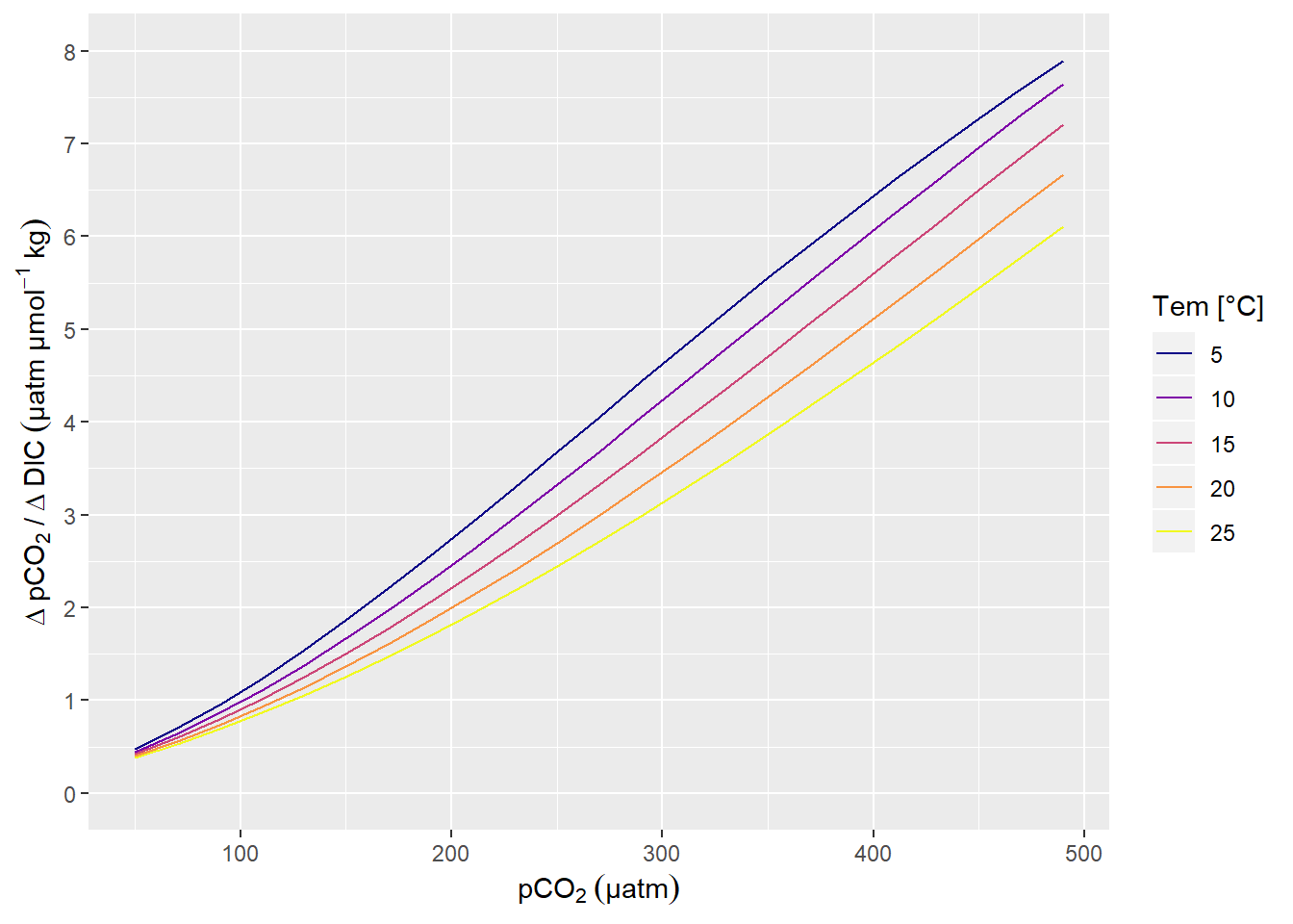
pCO2 sensitivity to changes in DIC.
rm(df, Tem, pCO2)Response time determination
HydroC sensor settings
The sensor was first run with a low power pump (1W). Later - and for most parts of the expedition - with a stronger (8W) pump. Pumps were switched between recordings (data file: SD_datafile_20180718_170417CO2-0618-001.txt):
- 2018-07-17;13:08:34
- 2018-07-17;13:08:35
Logging frequency for all measurement modes (Measure, Zero, Flush) was increased in two steps, It was:
10 sec for all recordings including SD_datafile_20180714_073641CO2-0618-001.txt
2 sec after change in SD_datafile_20180717_121052CO2-0618-001.txt at:
- 2018-07-14;07:52:02
- 2018-07-14;07:52:12
- 2018-07-14;07:52:14
1 sec after change in SD_datafile_20180718_170417CO2-0618-001 at:
- 2018-07-17;12:27:25
- 2018-07-17;12:27:27
- 2018-07-17;12:27:28
Model fitting
Response times were determined by fitting a nonlinear least-squares model with the nls function as described here by Douglas Watson.
- Flush period length: variable
- Flush period restricted to equilibration phase, avoiding initial gas mixing effects occuring at the start of each Flush period
- only completed Flush periods (duration > 500 sec) included
df <- read_csv(here::here("data/_merged_data_files",
                          "BloomSail_CTD_HydroC.csv"),
               col_types = cols(ID = col_character(),
                                pCO2_analog = col_double(),
                                pCO2 = col_double(),
                                Zero = col_factor(),
                                Flush = col_factor(),
                                Zero_ID = col_integer(),
                                deployment = col_integer(),
                                duration = col_double(),
                                mixing = col_character()))

df <- df %>%
  select(date_time, ID, dep, tem, Flush, pCO2, Zero_ID, duration, mixing)

df <- df %>%
  filter(Flush == 1, mixing == "equilibration")

df <- df %>%
  group_by(Zero_ID) %>%
  mutate(duration = duration- min(duration),
         max_duration = max(duration)) %>%
  ungroup() %>%
  filter(max_duration >= 500) %>%
  select(-max_duration)
An example plot for a nls model fitted to pCO2 observations during a Flush phase is shown below.
i <- unique(df$Zero_ID)[30]

df_ID <- df %>%
  filter(Zero_ID == i, duration <= 300)

fit <-
df_ID %>%
  nls(pCO2 ~ SSasymp(duration, yf, y0, log_alpha), data = .)

tau <- as.numeric(exp(-tidy(fit)[3,2]))
pCO2_end <- as.numeric(tidy(fit)[1,2])
pCO2_start <- as.numeric(tidy(fit)[2,2])
dpCO2 = pCO2_end - pCO2_start
mean_abs_resid <- mean(abs(resid(fit)))

augment(fit) %>%
  ggplot(aes(duration, pCO2))+
  geom_point()+
  geom_line(aes(y = .fitted))+
  geom_vline(xintercept = tau)+
  geom_hline(yintercept = pCO2_start + 0.63 *(dpCO2))+
  labs(y=expression(pCO[2]~(µatm)), x="Duration of Flush period (s)")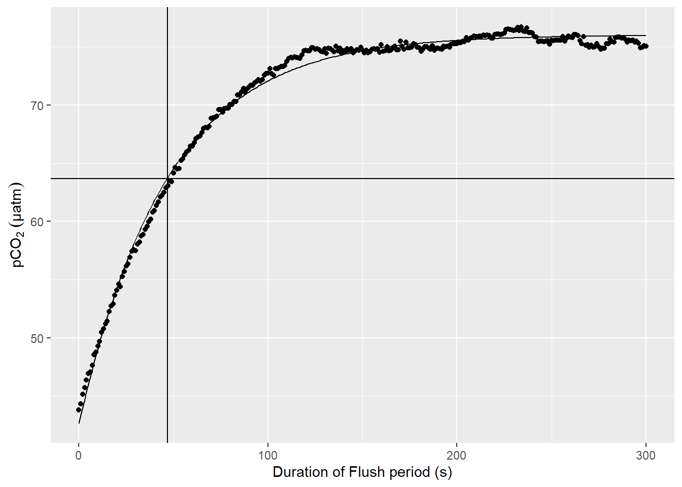
Example response time determination by non-linear least squares fit to the pCO2 recovery signal after zeroing. The vertical line indicates the determined response time tau. The horizontal line indicates 63% of the difference between start and final fitted pCO2.
rm(df_ID, fit, i, tau, dpCO2, pCO2_end, pCO2_start, mean_abs_resid)duration_intervals <- seq(150,500,50)As there was some speculation about the dependence of determined response times (\(\tau\)) on the chosen duration of the fit interval, the response time \(\tau\) was determined for all zeroings and for total durations of:
150, 200, 250, 300, 350, 400, 450, 500 secs
pdf(file=here::here("output/Plots/response_time",
    "RT_determination_pCO2_flushperiods_nls.pdf"), onefile = TRUE, width = 7, height = 4)

for (i in unique(df$Zero_ID)) {
  for (max_duration in duration_intervals) {

    df_ID <- df %>%
      filter(Zero_ID == i, duration <= max_duration)

    fit <-
      try(
      df_ID %>%
          nls(pCO2 ~ SSasymp(duration, yf, y0, log_alpha), data = .),
      TRUE)

    if (class(fit) == "nls"){

      tau <- as.numeric(exp(-tidy(fit)[3,2]))
      pCO2_end <- as.numeric(tidy(fit)[1,2])
      pCO2_start <- as.numeric(tidy(fit)[2,2])
      dpCO2 = pCO2_end - pCO2_start
      mean_abs_resid <- mean(abs(resid(fit))/pCO2_end)*100

      temp <- as_tibble(bind_cols(Zero_ID = i,
                                  duration = max_duration,
                                  date_time = mean(df_ID$date_time),
                                  dep = mean(df_ID$dep),
                                  tem = mean(df_ID$tem),
                                  pCO2 = pCO2_end,
                                  tau = tau,
                                  resid = mean_abs_resid))

      if (exists("tau_df")){tau_df <- bind_rows(tau_df, temp)}
        else {tau_df <- temp}

      if (mean_abs_resid > 1){warn <- "orange"}
        else {warn <- "black"}

      print(
      augment(fit) %>%
        ggplot(aes(duration, pCO2))+
        geom_point(col = warn)+
        geom_line(aes(y = .fitted))+
        geom_vline(xintercept = tau)+
        geom_hline(yintercept = pCO2_start + 0.63 *(dpCO2))+
        labs(y=expression(pCO[2]~(µatm)), x="Duration of Flush period (s)",
             title = paste("Zero_ID: ", i,
                           "Tau: ", round(tau,1),
                           "Mean absolute residual (%): ", round(mean_abs_resid, 2)))+
        xlim(0,600)
      )

    }


    else {

      temp <- as_tibble(bind_cols(Zero_ID = i,
                                  duration = max_duration,
                                  date_time = mean(df_ID$date_time),
                                  dep = mean(df_ID$dep),
                                  tem = mean(df_ID$tem),
                                  pCO2 = pCO2_end,
                                  tau = NaN,
                                  resid = NaN))

      if (exists("tau_df")){tau_df <- bind_rows(tau_df, temp)}
        else {tau_df <- temp}

      print(
      df_ID %>%
        ggplot(aes(duration, pCO2))+
        geom_point(col="red")+
        labs(y=expression(pCO[2]~(µatm)), x="Duration of Flush period (s)",
             title = paste("Zero_ID: ", i,
                           "nls model failed"))+
        xlim(0,600)
      )

    }
  }
}

dev.off()

rm(df_ID, fit, i, tau, dpCO2, pCO2_end, pCO2_start, temp, max_duration, mean_abs_resid, warn)

tau_df %>%
  write_csv(here::here("data/_summarized_data_files", "Tina_V_HydroC_response_times_all.csv"))

rm(tau_df, df)
A pdf with plots of all individual response time fits can be accessed here
tau_df <- read_csv(here::here("data/_summarized_data_files", "Tina_V_HydroC_response_times_all.csv"))

max_Zero_ID <- max(unique(tau_df[tau_df$date_time < ymd_hms("2018-07-17;13:08:34"),]$Zero_ID))

tau_df <- tau_df %>%
  mutate(pump_power = if_else(Zero_ID <= max_Zero_ID, "1W", "8W"))


# define subsetting parameters
resid_limit <- 1

# subset determined tau values by residual threshold
tau_resid <- tau_df %>%
  group_by(Zero_ID) %>%
  mutate(resid_max = max(resid, na.rm = TRUE)) %>%
  filter(resid_max < resid_limit) %>%
  select(-resid_max) %>%
  ungroup()

tau_resid_out <- tau_df %>%
  group_by(Zero_ID) %>%
  mutate(resid_max = max(resid, na.rm = TRUE)) %>%
  filter(resid_max > resid_limit) %>%
  select(-resid_max) %>%
  ungroup()

# Flush periods where model failure occured
tau_df %>%
  filter(is.na(resid)) %>%
  group_by(Zero_ID) %>%
  summarise(n()) %>%
  ungroup()

# Flush periods removed due to residual criterion
tau_resid_out %>%
  group_by(Zero_ID) %>%
  summarise(n()) %>%
  ungroup()

# mean tau of first RT determination
tau_resid %>%
  filter(Zero_ID == 2) %>%
  summarise(tau = mean(tau))

# mean tau of all RT determinations before pump switch, except first
tau_resid %>%
  filter(Zero_ID != 2, Zero_ID <= 20) %>%
  summarise(tau = mean(tau))

tau_resid <- tau_resid %>%
  filter(Zero_ID != 2)

# calculate some metrics for the subsetting
n_Zero_IDs <- tau_df %>%
  group_by(Zero_ID) %>%
  n_groups()
n_duration_intervals <- length(duration_intervals)
n_tau_max <- n_Zero_IDs * length(duration_intervals)
n_tau_total <- nrow(tau_df %>% filter(!is.na(resid)))
n_tau_resid <- nrow(tau_resid)

rm(df)
Outcome
General considerations
Estimated \(\tau\) values were only taken into account when stable environmental pCO2 levels were present. Absence of stable environmental pCO2 was assumed when the mean absolute fit residual was above 1 % of the final equilibrium pCO2. If one model fit (irrespective the chosen fit interval length) of a particular flush period did not match that criterion, the flush period was ignored. Usually, fits with the higher duration did not meet this criterion. For some unexplained reason the first \(\tau\) determination resulted in values about twice as high as all other Flush periods and was therefore removed as an outlier.
Metrics to characterize the fitting procedure include the number of:
- Flush periods: 75
- Duration intervals: 8
- Exercised response time fits: 600
- Succesful response times determinations: 576 (96)%
- \(\tau\)’s after removing groups of fits with high absolute fit residual: 408 (68 %)
It should be noted that all failed model fits occured in flush periods where the residual criterion was not meet by at least one other fit (i.e. fitting only failed under unstable conditions).
tau_df %>%
  ggplot(aes(resid))+
  geom_histogram()+
  facet_wrap(~duration, labeller = label_both)+
  geom_vline(xintercept = resid_limit)+
  labs(x=expression(Mean~absolute~residuals~("%"~of~equilibrium~pCO[2])))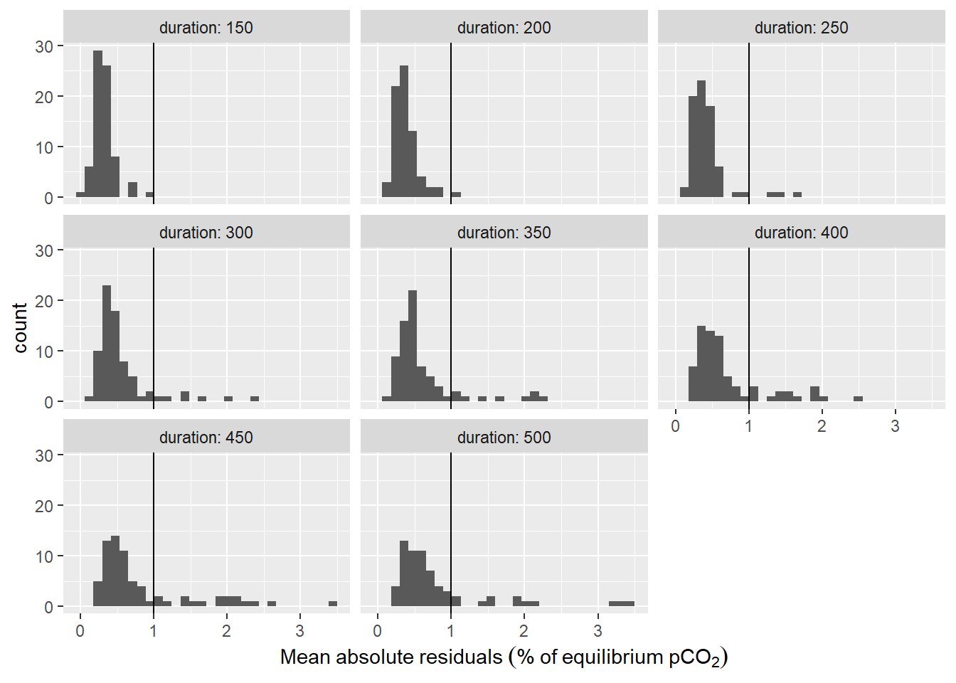
Histogram of residuals from fit displayed for the investigate durations of the fit interval. Vertical line represents the chosen threshold.
tau_resid %>%
  ggplot(aes(date_time, tau, col=dep, shape=pump_power))+
  geom_point()+
  scale_color_viridis_c(name="Depth (m)")+
  labs(y="Tau (sec)")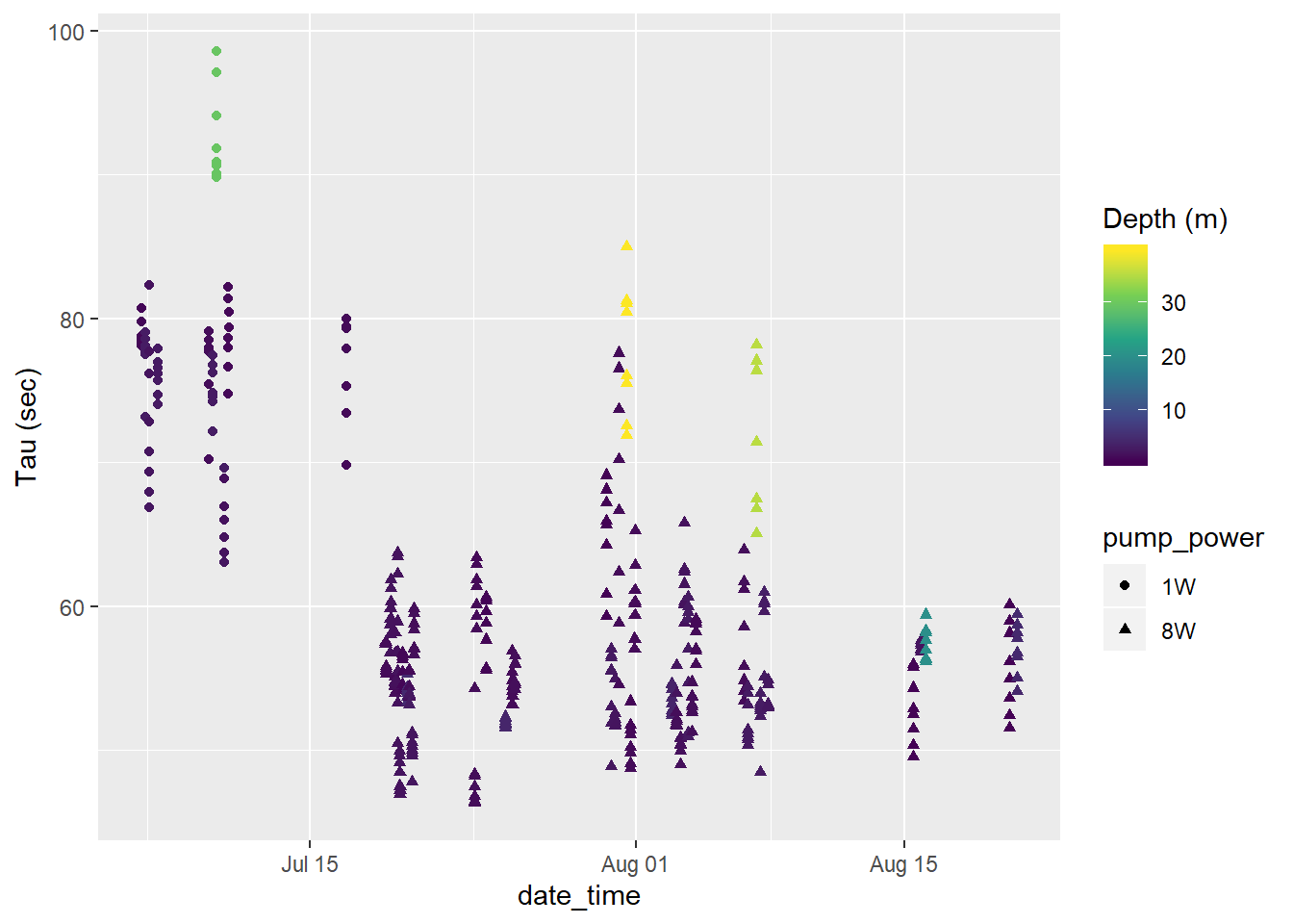
Tau for all Zeroings with color representing water depth.
Depth and temperature dependence
A temperature dependence of determined response times \(\tau\) was found, with similar slopes but different intercepts for both pumps used.
tau_resid %>%
  #filter(duration > 200, duration < 400) %>%
  ggplot(aes(tem, tau, col=dep))+
  geom_smooth(method = "lm")+
  geom_point()+
  scale_color_viridis_c(name="Depth (m)")+
  labs(y="Tau (sec)", x="Temp (deg C)")+
  facet_wrap(~pump_power)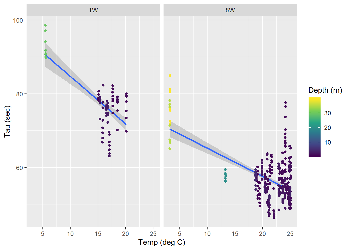
Tau as a function of temperature for all zeroings determined with low power (left) and strong (right) pump. Color represents the water depth.
For the response times determined near the surface (<10m, restricted temperature range), no clear temperature dependence of \(\tau\) was detected.
tau_resid %>%
  filter(dep < 10) %>%
  ggplot(aes(tem, tau, col=dep))+
  geom_smooth(method = "lm")+
  geom_point()+
  scale_color_viridis_c(name="Depth (m)")+
  labs(y="Tau (sec)", x="Tem (deg C)")+
  facet_wrap(~pump_power)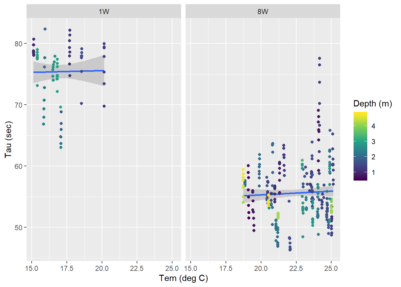
Surface tau (<10m) as a function of temperature for all zeroings determined with low power (left) and strong (right) pump. Color represents the water depth.
Fit interval length
No clear dependence of \(\tau\) on the length of the flushing period was found.
tau_resid %>%
  group_by(Zero_ID) %>%
  mutate(d_tau = tau - mean(tau)) %>%
  ggplot(aes(duration, d_tau))+
  geom_hline(yintercept = 0)+
  geom_smooth()+
  geom_point()+
  facet_wrap(~Zero_ID, ncol = 4, labeller = label_both)+
  labs(x="Duration (sec)", y="Deviation from mean tau (sec)")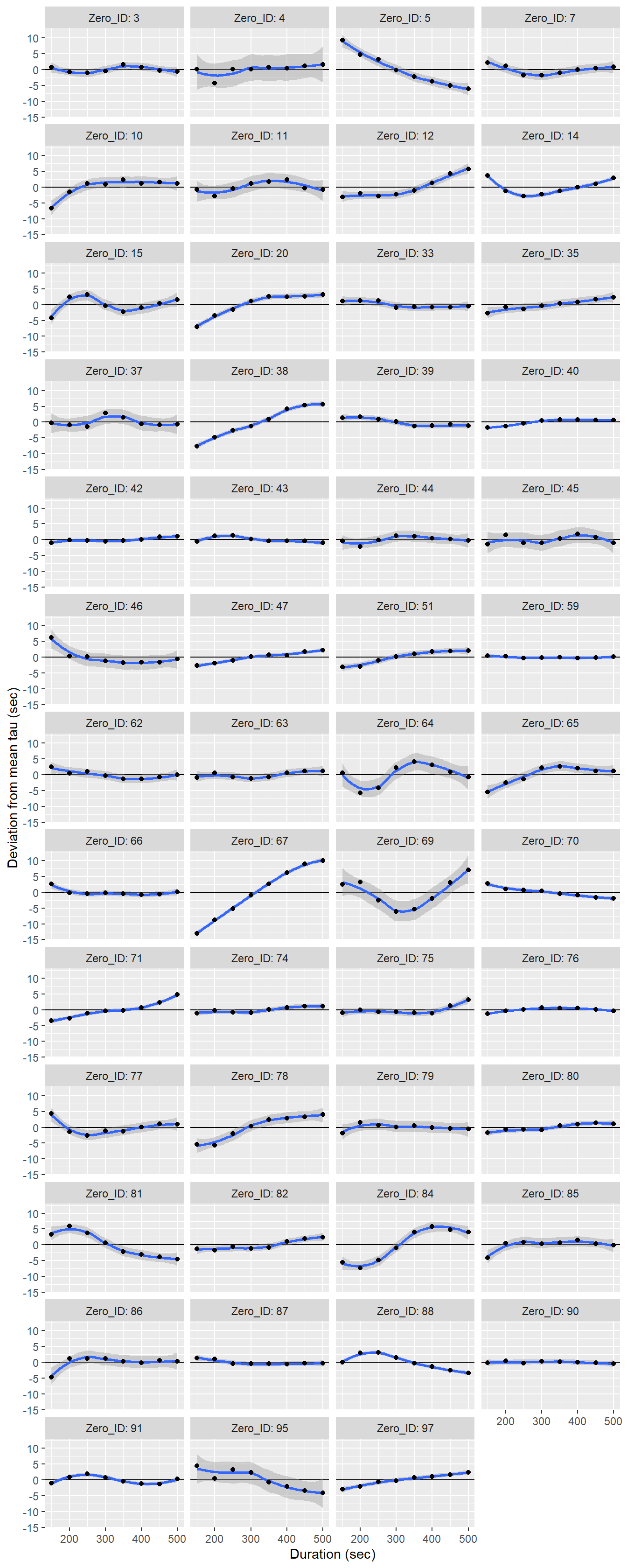
Determined tau values as a function of the fit interval duration, displayed individually for each flush period.
tau_resid %>%
  group_by(Zero_ID) %>%
  mutate(d_tau = tau - mean(tau)) %>%
  ggplot(aes(duration, d_tau, group=duration))+
  geom_violin()+
  geom_point()+
  labs(x="Duration (sec)", y="Deviation from mean tau (sec)")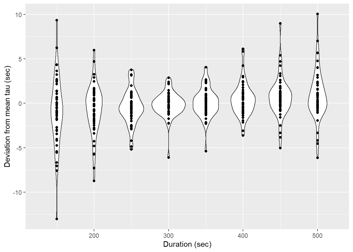
Determined tau values as a function of the fit interval duration, pooled for all flush period.
Mean response time fits
Finally, the mean response times are:
RT_mean <- tau_resid %>%
  group_by(pump_power) %>%
  summarise(tau = mean(tau))

RT_mean
# A tibble: 2 x 2
pump_power tau
<chr> <dbl>
1 1W 77.2
2 8W 56.6But we can also fit response times as a function of water temperature:
RT_fit <- tau_resid %>%
  group_by(pump_power) %>%
  do(fit = lm(tau ~ tem, data = .)) %>%
  tidy(fit) %>%
  select(pump_power, term, estimate) %>%
  spread(term, estimate)

RT_fit
# A tibble: 2 x 3
# Groups: pump_power [2]
pump_power `(Intercept)` tem
<chr> <dbl> <dbl>
1 1W 97.6 -1.29
2 8W 72.9 -0.763rm(list=setdiff(ls(), c("tau_resid", "RT_mean", "RT_fit")))Both response time estimated (constant mean vs T-dependent) will be used to correct the recorded pCO2 profiles.
Response time correction
Data preparation
Following tasks were performed to prepare data for the response time correction:
- Select only profiles
- Assign deployment periods with 1W- and 8W- pump
- Include manually derived meta-information about the profiling status
- Subset reference pCO2 recordings at the end of equilibration periods executed at constant depth
df <- read_csv(here::here("data/_merged_data_files",
                          "BloomSail_CTD_HydroC.csv"),
               col_types = cols(ID = col_character(),
                                pCO2_analog = col_double(),
                                pCO2 = col_double(),
                                Zero = col_factor(),
                                Flush = col_factor(),
                                Zero_ID = col_integer(),
                                deployment = col_integer(),
                                duration = col_double(),
                                mixing = col_character()))

# extract relevant parts

df <- df %>%
  select(date_time, ID, type, station, dep, sal, tem, Zero, Flush, pCO2, deployment, Zero_ID)

df <- df %>%
  filter(type == "P")

df <- df %>%
  group_by(ID, station) %>%
  mutate(duration = as.numeric(date_time - min(date_time)),
         pump_power = if_else(date_time < ymd_hms("2018-07-17;13:08:34"), "1W", "8W")) %>%
  arrange(date_time)
cast_dep <- df %>%
pivot_longer(c(dep, pCO2), names_to = "parameter", values_to = "value")
pdf(file=here::here("output/Plots/response_time",
"RT_exploration_depth-pCO2_timeseries_raw.pdf"), onefile = TRUE, width = 7, height = 4)
for(i_ID in unique(cast_dep$ID)){
for(i_station in unique(cast_dep$station)){
if (nrow(cast_dep %>% filter(ID == i_ID, station == i_station)) > 0){
print(
cast_dep %>%
filter(ID == i_ID,
station == i_station) %>%
ggplot(aes(duration, value))+
geom_point(size=0.5)+
scale_y_reverse()+
scale_x_continuous(breaks = seq(0,6000,100))+
labs(title = str_c("Date: ",i_ID," | Station: ",i_station))+
facet_grid(parameter~., scales = "free_y")+
theme_bw()
)
}
}
}
dev.off()
rm(cast_dep, i_station, i_ID)# Load profile meta data
meta <- read_csv(here::here("Data/_summarized_data_files",
"Tina_V_Sensor_meta.csv"),
col_types = cols(ID = col_character()))
# Merge data and meta information
df <- full_join(df, meta)
rm(meta)
# creating descriptive variables ------------------------------------------
df <- df %>%
mutate(phase = "standby",
phase = if_else(duration >= start & duration < down & !is.na(down) & !is.na(start), "down", phase),
phase = if_else(duration >= down & duration < lift & !is.na(lift) & !is.na(down ), "low", phase),
phase = if_else(duration >= lift & duration < up & !is.na(up ) & !is.na(lift ), "mid", phase),
phase = if_else(duration >= up & duration < end & !is.na(end ) & !is.na(up ), "up", phase))
df <- df %>%
select(-c(start, down, lift, up, end, comment))
df <- df %>%
filter(Zero == 0, Flush == 0)df_equi <- df %>%
filter(phase %in% c("mid")) %>%
group_by(ID, station, p_type, phase) %>%
top_n(5, row_number()) %>%
summarise(date_time = mean(date_time),
duration = mean(duration),
pCO2 = mean(pCO2, na.rm = TRUE),
dep = mean(dep, na.rm = TRUE)) %>%
ungroup()
df_equi %>%
write_csv(here::here("data/_merged_data_files",
"BloomSail_CTD_HydroC_reference_pCO2.csv"))cast_dep <- df %>%
pivot_longer(c(dep, pCO2), names_to = "parameter", values_to = "value")
cast_dep_equi <- df_equi %>%
pivot_longer(c(dep, pCO2), names_to = "parameter", values_to = "value")
max_duration <- round(max(cast_dep$duration)/1000,0)*1000
i_ID <- "180730"
i_station <- "P01"
cast_dep_equi_sub <- cast_dep_equi %>%
filter(ID == i_ID,
station == i_station)
cast_dep %>%
filter(ID == i_ID,
station == i_station) %>%
ggplot(aes(duration, value, col=phase))+
geom_point(size=0.5)+
geom_point(data = cast_dep_equi_sub, aes(duration, value), col="black")+
scale_y_reverse()+
scale_x_continuous(breaks = seq(0,6000,500))+
labs(title = str_c("Date: ",i_ID," | Station: ",i_station))+
facet_grid(parameter~., scales = "free_y")+
theme_bw()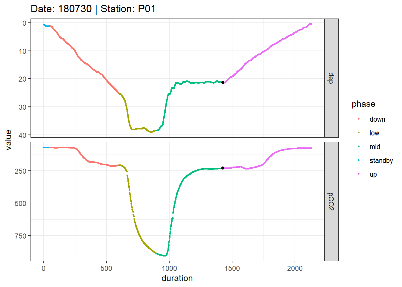
Example timeseries of profiling depth and pCO2. Colors represent manually assigned profiling phases. The black points represent reference data collected at the end of the mid equilibration period.
rm(cast_dep, cast_dep_equi, cast_dep_equi_sub, i_station, i_ID, max_duration)A pdf with all timeseries plots of profiling depth and pCO2 can be accessed here
cast_dep <- df %>%
  pivot_longer(c(dep, pCO2), names_to = "parameter", values_to = "value")

cast_dep_equi <- df_equi %>%
  pivot_longer(c(dep, pCO2), names_to = "parameter", values_to = "value")


max_duration <- round(max(cast_dep$duration)/1000,0)*1000

pdf(file=here::here("output/Plots/response_time",
    "RT_exploration_depth-pCO2_timeseries.pdf"), onefile = TRUE, width = 7, height = 4)

for(i_ID in unique(cast_dep$ID)){
  for(i_station in unique(cast_dep$station)){

    if (nrow(cast_dep %>% filter(ID == i_ID, station == i_station)) > 0){

        cast_dep_equi_sub <- cast_dep_equi %>%
        filter(ID == i_ID,
               station == i_station)

      print(

        cast_dep %>%
        filter(ID == i_ID,
               station == i_station) %>%
        ggplot(aes(duration, value, col=phase))+
        geom_point(size=0.5)+
        geom_point(data = cast_dep_equi_sub, aes(duration, value), col="black")+
        scale_y_reverse()+
        scale_x_continuous(breaks = seq(0,6000,500))+
        labs(title = str_c("Date: ",i_ID," | Station: ",i_station))+
        facet_grid(parameter~., scales = "free_y")+
        theme_bw()

      )

    }

  }
}

dev.off()

rm(cast_dep, cast_dep_equi, cast_dep_equi_sub, i_station, i_ID, max_duration)
Reponse time correction
The executed response time correction featured the following aspects:
- Correction according to Bittig et al. (2018, supplement)
- RT: Constant mean vs. T-dependent response times applied (both independently quantified for 1W- and 8W-pump)
- tau_factor: Factor ranging from 0.8 - 1.6 applied to determined tau values
- Post-smmoothing: 30 sec running mean (eg across 15 observations at 2 sec measurement frequency)
# Response time correction approach after Bittig --------------------------

RT_corr <- function(c1, c0, dt, tau) {
  ( 1 / ( 2* (( 1+(2*tau/dt) )^(-1) ))) * (c1 - (1-(2* (( 1+(2*tau/dt) )^(-1) ))) * c0)
}


# Assign mean response time (tau) values ----------------------------------------------

df_mean <- full_join(df, RT_mean)

df_mean <- df_mean %>%
  mutate(RT = "constant")

# Assign T-dependent response time (tau) values ----------------------------------------------

RT_fit <- RT_fit %>%
  rename(tau_intercept = `(Intercept)`, tau_slope=tem)

df_fit <- full_join(df, RT_fit)

df_fit <- df_fit %>%
  mutate(tau = tau_intercept + tau_slope *tem,
         RT = "T-dependent") %>%
  select(-tau_intercept, -tau_slope)

df_fit <- df_fit %>%
  mutate(RT = "T-dependent")


# Merge data sets with constand and T-dependent tau

df <- bind_rows(df_fit, df_mean)

rm(df_fit, df_mean)

# p1 <- df %>%
#   ggplot(aes(tau, dep, col=pump_power))+
#   geom_point()+
#   scale_y_reverse()
#
# p2 <- df %>%
#   ggplot(aes(tem, dep, col=pump_power))+
#   geom_point()+
#   scale_y_reverse()
#
# p1 | p2
#
# rm(p1, p2)


# Prepare data set for RT correction --------------------------------------

df <- df %>%
  group_by(RT) %>%
  arrange(date_time) %>%
  mutate(dt = as.numeric(as.character(date_time - lag(date_time)))) %>%
  ungroup()

# measurement frequency

freq <- df %>%
  filter(dt < 13) %>%
  group_by(ID) %>%
  summarise(dt_mean = round(mean(dt, na.rm = TRUE),0))

df <- full_join(df, freq)

# tau factors

df <- expand_grid(df, tau_factor = seq(0.8, 1.6, 0.2))

df <- df %>%
  mutate(tau_test = tau*tau_factor)


# Apply RT correction to entire data set

for(i_ID in unique(df$ID)){

#i_ID <- "180716"

  freq_sub <- freq %>% filter(ID == i_ID) %>% pull(dt_mean)

  window <- 30 / freq_sub
  rolling_mean   <- rollify(~mean(.x, na.rm = TRUE), window = window)

  df_sub <- df %>%
    filter(ID == i_ID) %>%
    group_by(station, RT, tau_factor) %>%
    mutate(pCO2_RT = RT_corr(pCO2, lag(pCO2), dt, tau_test),
           pCO2_RT = if_else(pCO2_RT %in% c(Inf, -Inf), NaN, pCO2_RT),
           window = window,
           pCO2_RT_mean = rolling_mean(pCO2_RT)
           #pCO2_RT_median = rolling_median(pCO2_RT)
           ) %>%
    ungroup()

  # time shift RT corrected data
  shift <- as.integer(as.character(window/2))

  df_sub <- df_sub %>%
    group_by(station, RT, tau_factor) %>%
    mutate(pCO2_RT_mean = lead(pCO2_RT_mean, shift)) %>%
    ungroup()


  if (exists("df_corr")){df_corr <- bind_rows(df_corr, df_sub)}
  else{df_corr <- df_sub}

  rm(df_sub, freq_sub, rolling_mean, shift, window)

}

df <- df_corr
rm(RT_corr, i_ID, freq, df_corr)

df %>%
 write_csv(here::here("data/_merged_data_files",
                      "BloomSail_CTD_HydroC_profiles_RT.csv"))
rm(df)
df <-
read_csv(here::here("data/_merged_data_files",
"BloomSail_CTD_HydroC_profiles_RT.csv"),
col_types = cols(ID = col_character(),
pCO2 = col_double(),
Zero = col_factor(),
Flush = col_factor(),
p_type = col_factor(),
Zero_ID = col_integer(),
deployment = col_integer(),
duration = col_double()))
i_ID <- "180730"
i_station <- "P01"
equi_cast <- df_equi %>%
filter(ID == i_ID,
station == i_station)
df %>%
filter(ID == i_ID,
station == i_station,
phase %in% c("up", "down")) %>%
ggplot()+
geom_path(aes(pCO2, dep, linetype = phase, col="raw"))+
geom_path(aes(pCO2_RT_mean, dep, linetype = phase, col="corrected"))+
geom_point(data = equi_cast, aes(pCO2, dep))+
scale_y_reverse()+
scale_color_brewer(palette = "Set1", name="")+
labs(y="Depth [m]", title = str_c("Date: ",i_ID," | Station: ",i_station))+
theme_bw()+
facet_grid(tau_factor~RT, labeller = label_both)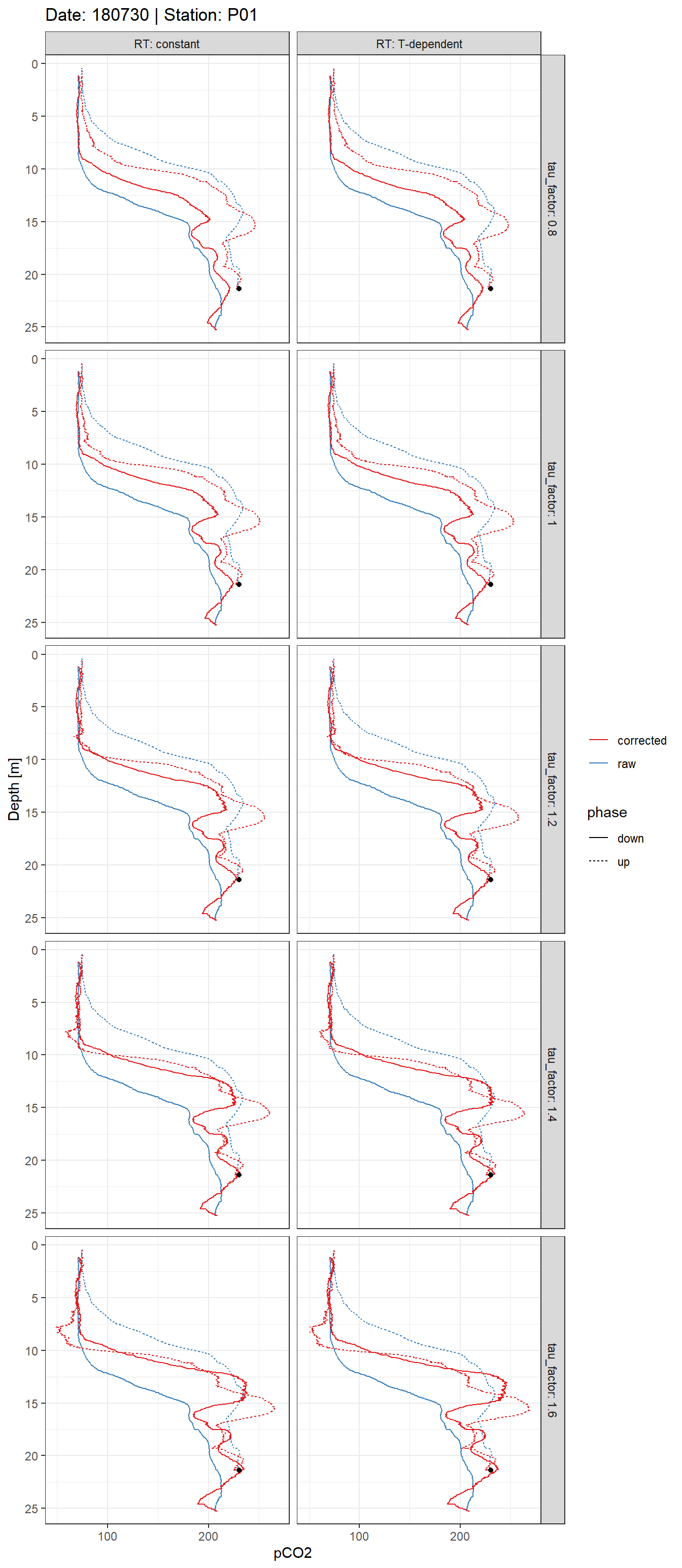
Example plot of response time corrected and raw pCO2 profiles. Panels highlight the effect of constant vs T-dependent tau estimates (columns) and the optimization by applying a constant factor (rows).
rm(equi_cast)A pdf with all timeseries plots of profiling depth and pCO2 can be accessed here
pdf(file=here::here("output/Plots/response_time",
    "RT_correction_pCO2_profiles.pdf"), onefile = TRUE, width = 7, height = 11)

for(i_ID in unique(df$ID)){
  for(i_station in unique(df$station)){

    if (nrow(df %>% filter(ID == i_ID, station == i_station)) > 0){

      equi_cast <- df_equi %>%
        filter(ID == i_ID,
               station == i_station)

      print(

  df %>%
    filter(ID == i_ID,
           station == i_station,
           phase %in% c("up", "down")) %>%
    ggplot()+
    geom_path(aes(pCO2, dep, linetype = phase, col="raw"))+
    geom_path(aes(pCO2_RT_mean, dep, linetype = phase, col="corrected"))+
    geom_point(data = equi_cast, aes(pCO2, dep))+
    scale_y_reverse()+
    scale_color_brewer(palette = "Set1", name="")+
    labs(y="Depth [m]", title = str_c("Date: ",i_ID," | Station: ",i_station))+
    theme_bw()+
    facet_grid(tau_factor~RT, labeller = label_both)

      )

    }

  }
}

dev.off()

rm(equi_cast)
Diagnosis and conclusion
In the following, the success of the response time correction is assessed through the offset between the downcast and:
- upcast
- pCO2 reference value recorded at the end of an equilibration period during the upcast
The offset comparison requires to discretize the depth recording. Depth intervals of 1m were chosen.
First, we take a look at individual profiles.
Down- vs upcast
# pCO2 offset up - down cast

RT_diff <- df %>%
  filter(phase %in% c("down", "up")) %>%
  mutate(dep_int = as.numeric(as.character( cut(dep, seq(0,40,2),seq(1,39,2)))),
         tau_factor = as.factor(tau_factor)) %>%
  select(ID, station, RT, tau_factor, p_type, dep_int, phase, pCO2, pCO2_RT_mean) %>%
  group_by(ID, station, RT, tau_factor, p_type, dep_int, phase) %>%
  summarise_all("mean", na.rm = TRUE) %>%
  ungroup() %>%
  pivot_longer(cols = c(pCO2, pCO2_RT_mean), names_to = "correction") %>%
  pivot_wider(names_from = phase, values_from = value) %>%
  mutate(d_pCO2 = up - down,
         mean_pCO2 = (down + up)/2,
         d_pCO2_rel = 100 * d_pCO2 / mean_pCO2)

# descritize depth recordings of equilibrated pCO2 values

equi_diff <- df_equi %>%
  mutate(dep_int = as.numeric(as.character( cut(dep, seq(0,40,2),seq(1,39,2))))) %>%
  select(ID, station, dep_int, pCO2_equi=pCO2)


RT_diff %>%
 write_csv(here::here("data/_merged_data_files",
                      "BloomSail_CTD_HydroC_profiles_RT_cast-offset.csv"))

equi_diff %>%
 write_csv(here::here("data/_merged_data_files",
                      "BloomSail_CTD_HydroC_profiles_RT_reference-offset.csv"))
RT_diff <-
read_csv(here::here("data/_merged_data_files",
"BloomSail_CTD_HydroC_profiles_RT_cast-offset.csv"),
col_types = cols(ID = col_character()))
equi_diff <-
read_csv(here::here("data/_merged_data_files",
"BloomSail_CTD_HydroC_profiles_RT_reference-offset.csv"),
col_types = cols(ID = col_character()))
i_ID <- "180730"
i_station <- "P01"
equi_diff_sub <- equi_diff %>%
filter(ID == i_ID,
station == i_station)
RT_diff %>%
filter(ID == i_ID,
station == i_station) %>%
arrange(dep_int) %>%
ggplot()+
geom_path(aes(down, dep_int, col=correction, linetype="down"))+
geom_path(aes(up, dep_int, col=correction, linetype ="up"))+
geom_point(data = equi_diff_sub, aes(pCO2_equi, dep_int))+
scale_y_reverse(breaks=seq(0,40,2))+
scale_linetype(name="cast")+
scale_color_brewer(palette = "Set1", direction = -1)+
labs(y="Depth [m]", title = str_c("Date: ",i_ID," | Station: ",i_station))+
theme_bw()+
facet_grid(tau_factor~RT, labeller = label_both)
Example plot of discretized, response time corrected and raw pCO2 profiles. Panels highlight the effect of constant vs T-dependent tau estimates (columns) and the optimization by applying a constant factor (rows). The black point indicates the reference pCO2 value.
rm(equi_diff_sub)A pdf with all discretized pCO2 profiles can be assessed here
pdf(file=here::here("output/Plots/response_time",
    "RT_correction_pCO2_profiles_discrete.pdf"), onefile = TRUE, width = 7, height = 11)

for(i_ID in unique(RT_diff$ID)){
  for(i_station in unique(RT_diff$station)){

    if (nrow(RT_diff %>% filter(ID == i_ID, station == i_station)) > 0){


        equi_diff_sub <- equi_diff %>%
        filter(ID == i_ID,
               station == i_station)

      print(

      RT_diff %>%
        filter(ID == i_ID,
               station == i_station) %>%
        arrange(dep_int) %>%
        ggplot()+
        geom_path(aes(down, dep_int, col=correction, linetype="down"))+
        geom_path(aes(up, dep_int, col=correction, linetype ="up"))+
        geom_point(data = equi_diff_sub, aes(pCO2_equi, dep_int))+
        scale_y_reverse(breaks=seq(0,40,2))+
        scale_linetype(name="cast")+
        scale_color_brewer(palette = "Set1", direction = -1)+
        labs(y="Depth [m]", title = str_c("Date: ",i_ID," | Station: ",i_station))+
        theme_bw()+
        facet_grid(tau_factor~RT, labeller = label_both)

      )

      rm(equi_diff_sub)
    }

  }
}

dev.off()
i_ID <- "180730"
i_station <- "P01"
RT_diff %>%
filter(ID == i_ID,
station == i_station,
correction == "pCO2_RT_mean") %>%
arrange(dep_int) %>%
ggplot(aes(d_pCO2, dep_int, col=as.factor(tau_factor)))+
geom_path()+
geom_point()+
scale_y_reverse(breaks=seq(0,40,2))+
scale_color_discrete(name="tau factor")+
labs(x = "delta pCO2 [µatm]", y="Depth [m]", title = str_c("Date: ",i_ID," | Station: ",i_station))+
geom_vline(xintercept = 0)+
geom_vline(xintercept = c(-10,10), col="red")+
theme_bw()+
facet_wrap(~RT, labeller = label_both)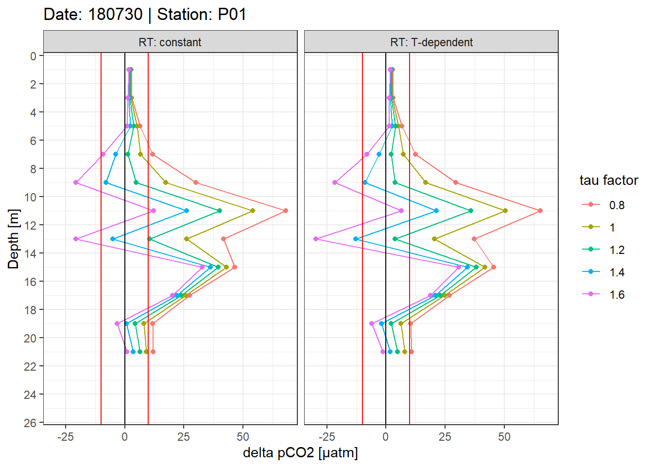
Example plot of absolute pCO2 offset profiles. Panels highlight the effect of constant vs T-dependent tau estimates. Colour indicates the optimization by applying a constant factor to tau. Vertical red lines mark an arbitray 10µatm pCO2 threshold.
pdf(file=here::here("output/Plots/response_time",
    "RT_correction_delta_pCO2_absolute_profiles_discrete.pdf"), onefile = TRUE, width = 7, height = 7)

for(i_ID in unique(RT_diff$ID)){
  for(i_station in unique(RT_diff$station)){

    if (nrow(RT_diff %>% filter(ID == i_ID, station == i_station)) > 0){

      print(

      RT_diff %>%
        filter(ID == i_ID,
               station == i_station,
               correction == "pCO2_RT_mean") %>%
        arrange(dep_int) %>%
        ggplot(aes(d_pCO2, dep_int, col=as.factor(tau_factor)))+
        geom_path()+
        geom_point()+
        scale_y_reverse(breaks=seq(0,40,2))+
        scale_color_discrete(name="tau factor")+
        labs(x = "delta pCO2 [µatm]", y="Depth [m]", title = str_c("Date: ",i_ID," | Station: ",i_station))+
        geom_vline(xintercept = 0)+
        geom_vline(xintercept = c(-10,10), col="red")+
        theme_bw()+
        facet_wrap(~RT, labeller = label_both)

      )

    }

  }
}

dev.off()
A pdf with all absolute pCO2 offset profiles can be assessed here
i_ID <- "180730"
i_station <- "P01"

      RT_diff %>%
        filter(ID == i_ID,
               station == i_station,
               correction == "pCO2_RT_mean") %>%
        arrange(dep_int) %>%
        ggplot(aes(d_pCO2_rel, dep_int, col=as.factor(tau_factor)))+
        geom_path()+
        geom_point()+
        scale_y_reverse(breaks=seq(0,40,2))+
        scale_color_discrete(name="tau factor")+
        labs(x = "delta pCO2 [% of absolute value]", y="Depth [m]", title = str_c("Date: ",i_ID," | Station: ",i_station))+
        geom_vline(xintercept = 0)+
        geom_vline(xintercept = c(-10,10), col="red")+
        theme_bw()+
        facet_wrap(~RT, labeller = label_both)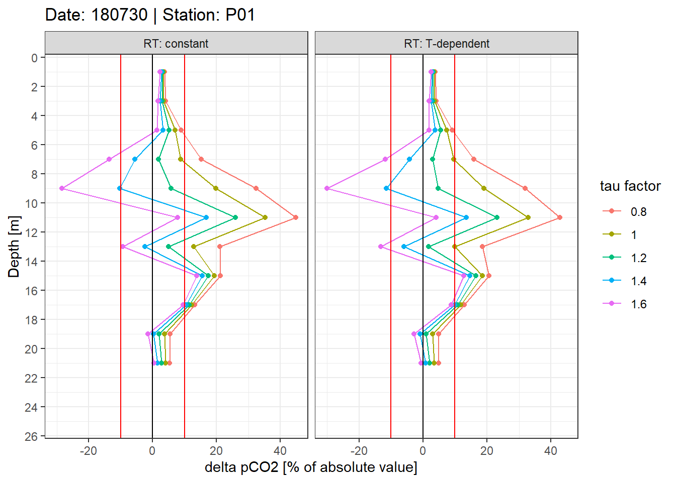
Example plot of relative offset pCO2 profiles. Panels highlight the effect of constant vs T-dependent tau estimates. Colour indicates the optimization by applying a constant factor to tau. Vertical red lines mark an arbitray 10% threshold.
A pdf with all relative pCO2 offset profiles can be assessed here
pdf(file=here::here("output/Plots/response_time",
    "RT_correction_delta_pCO2_relative_profiles_discrete.pdf"), onefile = TRUE, width = 7, height = 7)

for(i_ID in unique(RT_diff$ID)){
  for(i_station in unique(RT_diff$station)){

    if (nrow(RT_diff %>% filter(ID == i_ID, station == i_station)) > 0){

      print(

      RT_diff %>%
        filter(ID == i_ID,
               station == i_station,
               correction == "pCO2_RT_mean") %>%
        arrange(dep_int) %>%
        ggplot(aes(d_pCO2_rel, dep_int, col=as.factor(tau_factor)))+
        geom_path()+
        geom_point()+
        scale_y_reverse(breaks=seq(0,40,2))+
        scale_color_discrete(name="tau factor")+
        labs(x = "delta pCO2 [% of absolute value]", y="Depth [m]", title = str_c("Date: ",i_ID," | Station: ",i_station))+
        geom_vline(xintercept = 0)+
        geom_vline(xintercept = c(-10,10), col="red")+
        theme_bw()+
        facet_wrap(~RT, labeller = label_both)

      )

    }

  }
}

dev.off()
Downcast vs reference value
equi_RT_diff <- full_join(RT_diff, equi_diff) %>%
  filter(!is.na(pCO2_equi)) %>%
  mutate(d_pCO2_equi = down - pCO2_equi)
equi_RT_diff %>%
filter(RT == "T-dependent", tau_factor == 1.2, correction=="pCO2_RT_mean") %>%
ggplot(aes(pCO2_equi, d_pCO2_equi))+
geom_hline(yintercept = 0)+
geom_point()+
labs(x="Reference pCO2 [µatm]", y="Offset downcast to reference pCO2 [µatm]")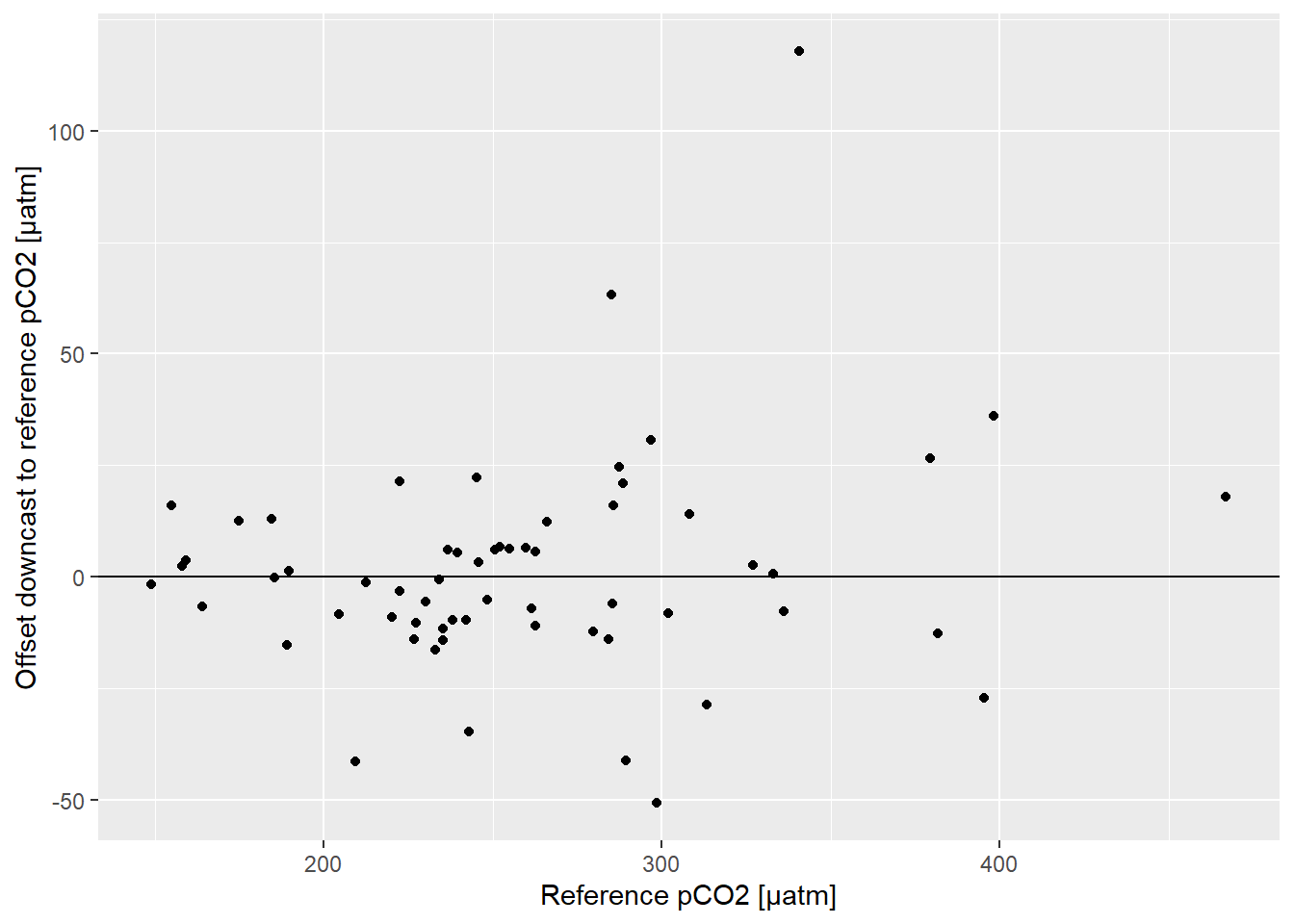
Offset between pCO2 downcast and upcast reference value as a function of absolute pCO2. (T-dependent tau estimates, tau factor: 1.2.
equi_RT_diff %>%
  ggplot(aes(as.factor(tau_factor), d_pCO2_equi, fill=correction))+
  geom_hline(yintercept = 0)+
  geom_violin()+
  labs(y = "delta pCO2 from reference [µatm]", y="Depth [m]")+
  scale_fill_brewer(palette = "Set1")+
  facet_wrap(~RT, labeller = label_both)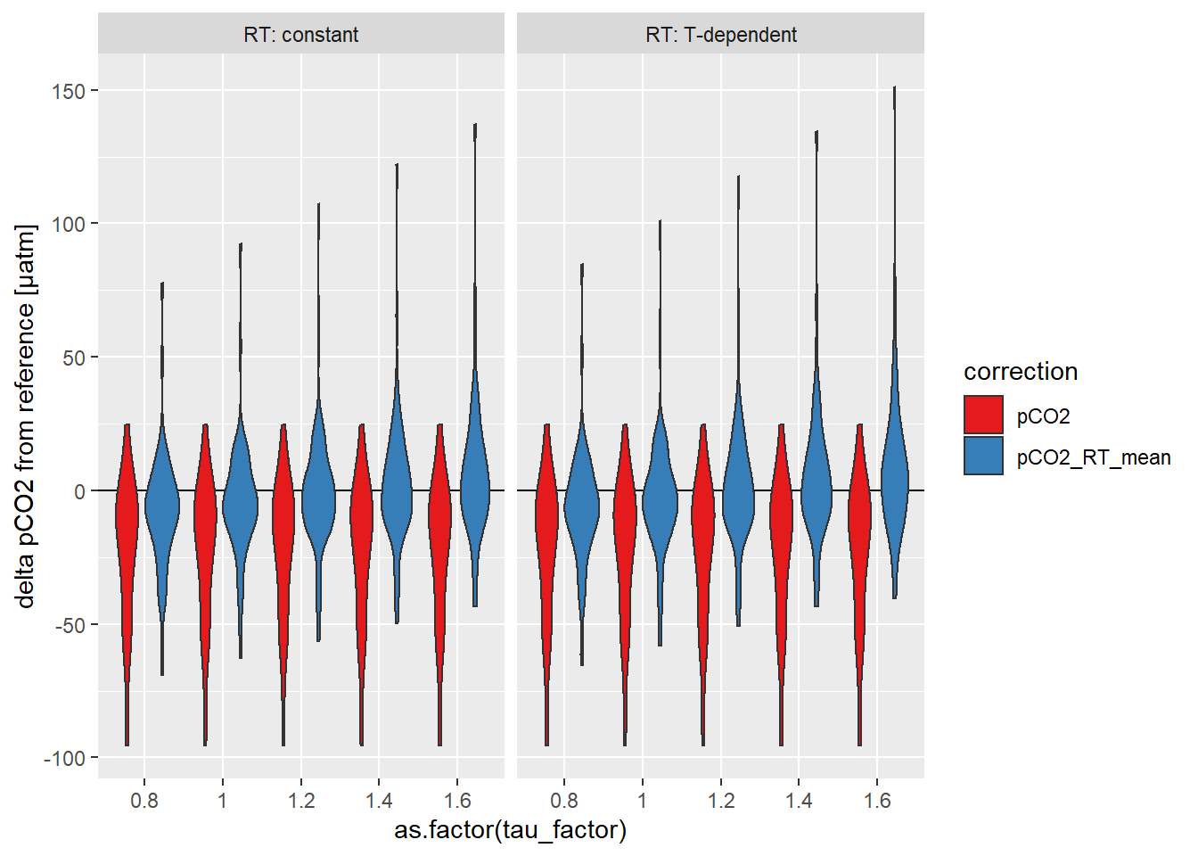
Offset between pCO2 downcast and upcast reference value. Panels highlight the effect of constant vs T-dependent tau estimates. Colour distinguish raw and corrected offsets.
Summary metrics
In order to decide, which conditions resulted in the best response correction, all profiles were pooled and some metrics derived.
RT_diff_20 <- RT_diff %>%
  group_by(ID, station) %>%
  filter(!any(is.na(d_pCO2))) %>%
  ungroup()

RT_diff_sum <- RT_diff_20 %>%
  filter(dep_int <= 20) %>%
  group_by(RT, tau_factor, dep_int, correction, p_type) %>%
  summarise(mean = mean(d_pCO2),
            mean_abs = mean(abs(d_pCO2)),
            mean_rel = mean(d_pCO2_rel, na.rm = TRUE),
            mean_rel_abs = mean(abs(d_pCO2_rel), na.rm = TRUE)) %>%
  ungroup() %>%
  pivot_longer(cols = 6:9, names_to = "estimate", values_to = "dpCO2")


equi_RT_diff_sum <- equi_RT_diff %>%
  group_by(correction, RT, tau_factor) %>%
  summarise(d_pCO2_equi = mean(d_pCO2_equi, na.rm = TRUE),
            d_pCO2_equi_abs = mean(abs(d_pCO2_equi), na.rm = TRUE)) %>%
  ungroup()
equi_RT_diff_sum %>%
ggplot(aes(tau_factor, d_pCO2_equi, col=RT, shape=correction, linetype=correction))+
geom_hline(yintercept = 0)+
geom_smooth(method = "lm")+
geom_point()+
labs(y = "Mean delta pCO2 from reference [µatm]")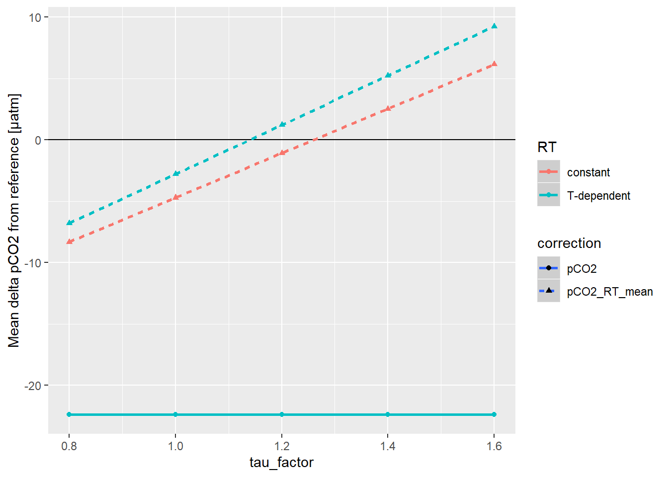
Mean pCO2 offset from reference values as a function of the factor applied to tau.
equi_RT_diff_sum %>%
  ggplot(aes(tau_factor, d_pCO2_equi_abs, col=RT, shape=correction, linetype=correction))+
  geom_hline(yintercept = 0)+
  stat_smooth(method = "lm", formula = y ~ x + I(x^2), se=FALSE)+
  geom_point()+
  labs(y = "Mean delta pCO2 from reference [µatm]")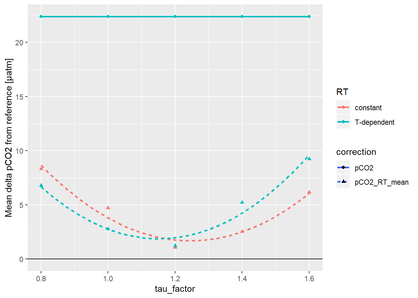
Mean pCO2 offset from reference values as a function of the factor applied to tau.
fit_factor_ref <- equi_RT_diff_sum %>%
  filter(correction == "pCO2_RT_mean") %>%
  group_by(RT) %>%
  do(fit = lm(d_pCO2_equi ~ tau_factor, data = .)) %>%
  tidy(fit) %>%
  select(RT, term, estimate) %>%
  spread(term, estimate)
RT_diff_sum %>%
filter(correction == "pCO2_RT_mean") %>%
ggplot()+
geom_path(aes(dpCO2, dep_int, col=as.factor(tau_factor)))+
scale_y_reverse()+
coord_cartesian(xlim = c(-30,30))+
geom_vline(xintercept = 0)+
theme_bw()+
geom_hline(yintercept = 20)+
geom_vline(xintercept = 0)+
geom_vline(xintercept = c(-10,10), col="red")+
facet_grid(estimate~RT*p_type)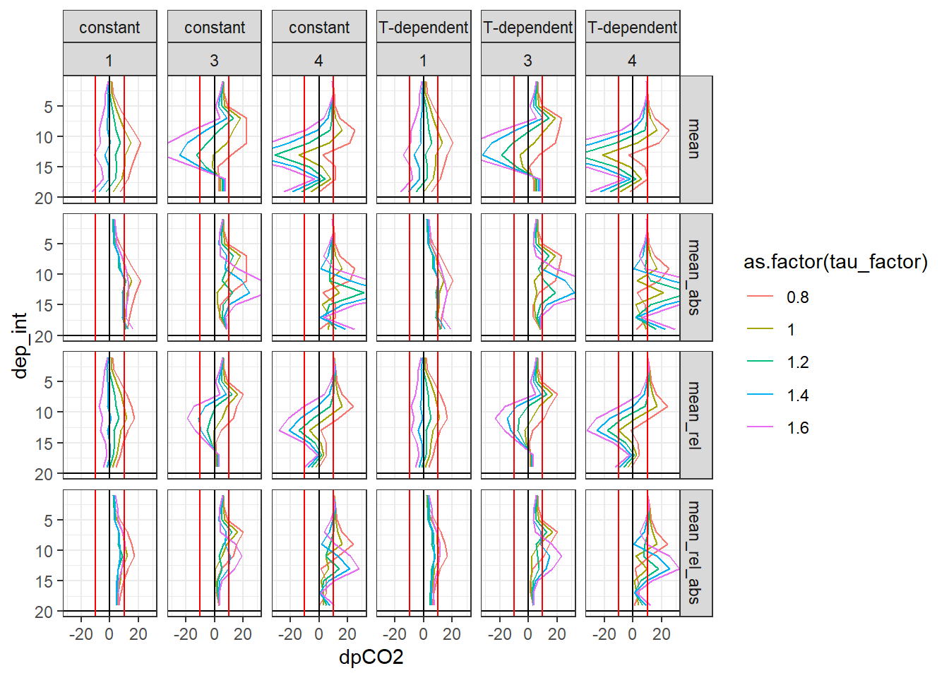
RT_diff_20 %>%
  ggplot(aes(as.factor(tau_factor), d_pCO2, fill=correction))+
  geom_violin()+
  geom_hline(yintercept = 0)+
  theme_bw()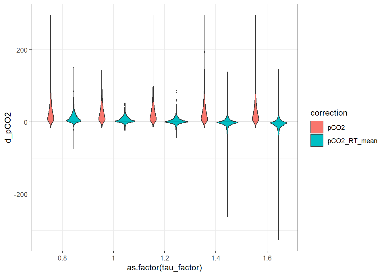
RT_diff_sum %>%
  filter(dep_int < 20, p_type == 1) %>%
  group_by(RT, estimate, correction, tau_factor) %>%
  summarise(mean_dpCO2 = mean(dpCO2)) %>%
  ungroup() %>%
  filter(correction == "pCO2_RT_mean") %>%
  ggplot(aes(tau_factor, mean_dpCO2, col=RT))+
  geom_point()+
  geom_hline(yintercept = 0)+
  stat_smooth(method = "lm", formula = y ~ x + I(x^2), se=FALSE)+
  facet_grid(~estimate)+
  theme_bw()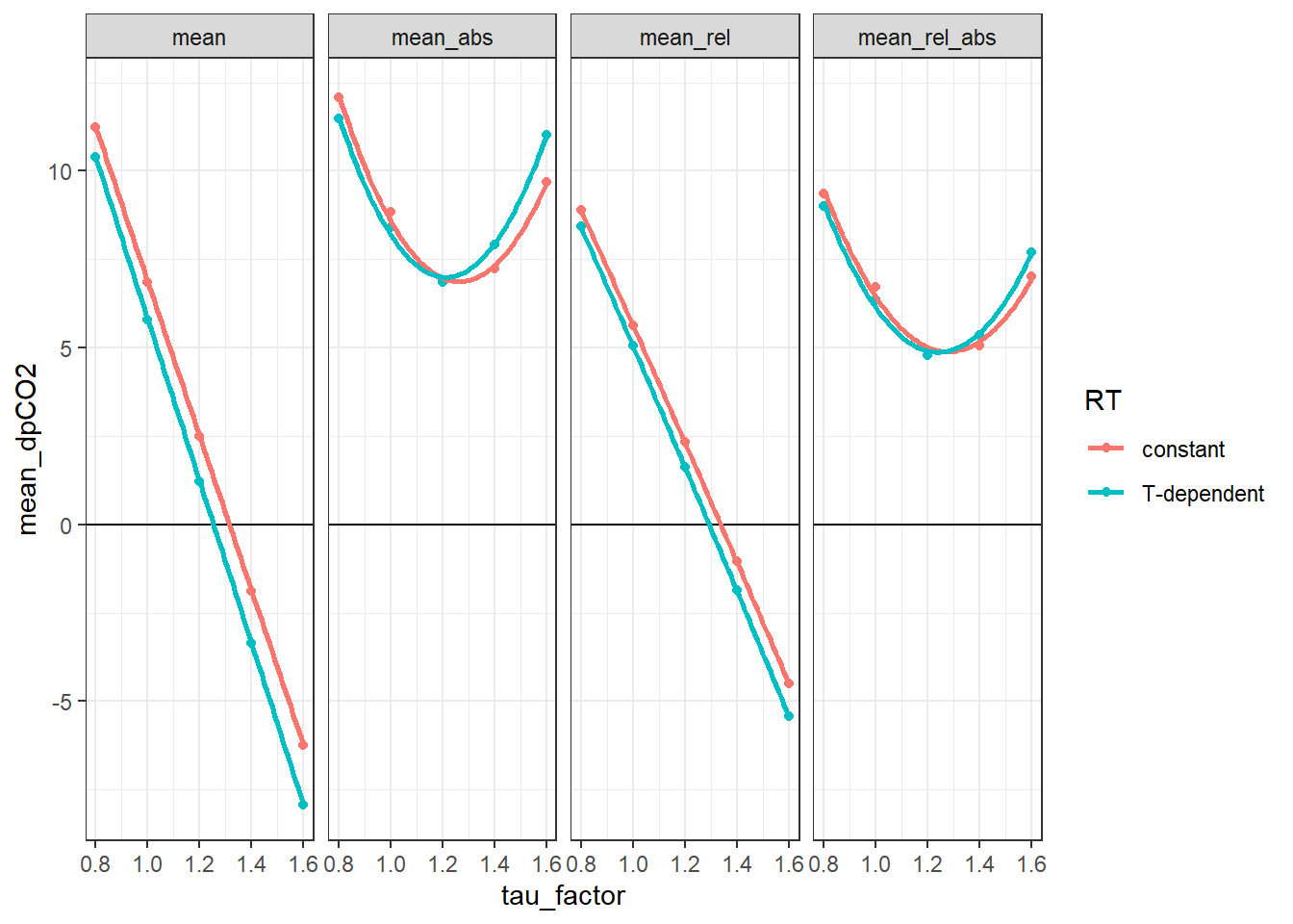
Open tasks / questions
- Check why type 2, 3, and 4 profiles exceed 10 µatm absolute mean pCO2 deviation at depth > 10m
- Check whether irregular profiles can be excluded from response time optimization
- Compare Contros and own response time estimates
- Compare differnt response time correction methods (Bittig vs. Fiedler, Miloshevich, Fietzek)
- Check results from field response time experiment (high zeroing frequency)
sessionInfo()R version 3.5.0 (2018-04-23)
Platform: x86_64-w64-mingw32/x64 (64-bit)
Running under: Windows 10 x64 (build 17763)
Matrix products: default
locale:
[1] LC_COLLATE=English_United States.1252
[2] LC_CTYPE=English_United States.1252
[3] LC_MONETARY=English_United States.1252
[4] LC_NUMERIC=C
[5] LC_TIME=English_United States.1252
attached base packages:
[1] stats graphics grDevices utils datasets methods base
other attached packages:
[1] patchwork_1.0.0 tibbletime_0.1.3 lubridate_1.7.4
[4] broom_0.5.2 data.table_1.12.6 seacarb_3.2.12
[7] oce_1.1-1 gsw_1.0-5 testthat_2.2.1
[10] forcats_0.4.0 stringr_1.4.0 dplyr_0.8.3
[13] purrr_0.3.3 readr_1.3.1 tidyr_1.0.0
[16] tibble_2.1.3 ggplot2_3.2.1 tidyverse_1.3.0
loaded via a namespace (and not attached):
[1] Rcpp_1.0.2 here_0.1 lattice_0.20-35
[4] utf8_1.1.4 assertthat_0.2.1 zeallot_0.1.0
[7] rprojroot_1.3-2 digest_0.6.22 plyr_1.8.4
[10] R6_2.4.0 cellranger_1.1.0 backports_1.1.5
[13] reprex_0.3.0 evaluate_0.14 highr_0.8
[16] httr_1.4.1 pillar_1.4.2 rlang_0.4.1
[19] lazyeval_0.2.2 readxl_1.3.1 rstudioapi_0.10
[22] rmarkdown_1.17 labeling_0.3 munsell_0.5.0
[25] compiler_3.5.0 httpuv_1.5.2 modelr_0.1.5
[28] xfun_0.10 pkgconfig_2.0.3 htmltools_0.4.0
[31] tidyselect_0.2.5 workflowr_1.5.0 fansi_0.4.0
[34] viridisLite_0.3.0 crayon_1.3.4 dbplyr_1.4.2
[37] withr_2.1.2 later_1.0.0 grid_3.5.0
[40] nlme_3.1-137 jsonlite_1.6 gtable_0.3.0
[43] lifecycle_0.1.0 DBI_1.0.0 git2r_0.26.1
[46] magrittr_1.5 scales_1.0.0 cli_1.1.0
[49] stringi_1.4.3 reshape2_1.4.3 fs_1.3.1
[52] promises_1.1.0 xml2_1.2.2 generics_0.0.2
[55] vctrs_0.2.0 RColorBrewer_1.1-2 tools_3.5.0
[58] glue_1.3.1 hms_0.5.2 yaml_2.2.0
[61] colorspace_1.4-1 rvest_0.3.5 knitr_1.25
[64] haven_2.2.0