CT dynamics
Jens Daniel Müller
26 March, 2020
Last updated: 2020-03-26
Checks: 7 0
Knit directory: BloomSail/
This reproducible R Markdown analysis was created with workflowr (version 1.6.0). The Checks tab describes the reproducibility checks that were applied when the results were created. The Past versions tab lists the development history.
Great! Since the R Markdown file has been committed to the Git repository, you know the exact version of the code that produced these results.
Great job! The global environment was empty. Objects defined in the global environment can affect the analysis in your R Markdown file in unknown ways. For reproduciblity it’s best to always run the code in an empty environment.
The command set.seed(20191021) was run prior to running the code in the R Markdown file. Setting a seed ensures that any results that rely on randomness, e.g. subsampling or permutations, are reproducible.
Great job! Recording the operating system, R version, and package versions is critical for reproducibility.
Nice! There were no cached chunks for this analysis, so you can be confident that you successfully produced the results during this run.
Great job! Using relative paths to the files within your workflowr project makes it easier to run your code on other machines.
Great! You are using Git for version control. Tracking code development and connecting the code version to the results is critical for reproducibility. The version displayed above was the version of the Git repository at the time these results were generated.
Note that you need to be careful to ensure that all relevant files for the analysis have been committed to Git prior to generating the results (you can use wflow_publish or wflow_git_commit). workflowr only checks the R Markdown file, but you know if there are other scripts or data files that it depends on. Below is the status of the Git repository when the results were generated:
Ignored files:
    Ignored:    .Rhistory
    Ignored:    .Rproj.user/
    Ignored:    data/Finnmaid_2018/
    Ignored:    data/GETM/
    Ignored:    data/Maps/
    Ignored:    data/Ostergarnsholm/
    Ignored:    data/TinaV/
    Ignored:    data/_merged_data_files/
    Ignored:    data/_summarized_data_files/
Note that any generated files, e.g. HTML, png, CSS, etc., are not included in this status report because it is ok for generated content to have uncommitted changes.
There are no past versions. Publish this analysis with wflow_publish() to start tracking its development.
library(tidyverse)
library(patchwork)
library(seacarb)
library(metR)
library(scico)
# library(cmocean)
# library(broom)
# library(lubridate)
# library(tibbletime)
1 Sensor data
Profile data are prepared by:
- Ignoring those made on June 16 (pCO2 sensor not in operation)
- Removing HydroC Flush and Zeroing periods
- Selecting only continous downcast periods
- Gridding profiles to 1m depth intervals
- Discarding profiles with 3 or more observation missing within upper 20m
- assigning mean date_time_ID value to all profiles belonging to one cruise
- discarding “coastal” station P01, P13, P14
- Restricting profiles to upper 25m
Please note that:
- The label ID represents the start date of the cruise (“YYMMDD”), not the exact mean sampling date
1.1 pCO2 profile overview
ts <-
 read_csv(here::here("data/_merged_data_files",
                      "BloomSail_CTD_HydroC_track_RT.csv"),
               col_types = cols(ID = col_character(),
                                pCO2_analog = col_double(),
                                pCO2 = col_double(),
                                Zero = col_character(),
                                Flush = col_character(),
                                mixing = col_character(),
                                Zero_ID = col_integer(),
                                deployment = col_integer(),
                                lon = col_double(),
                                lat = col_double(),
                                pCO2_RT = col_double()))


# Filter relevant rows and columns

ts_profiles <- ts %>%
  filter(type == "P",
         Flush == "0",
         Zero == "0",
         !ID %in% c("180616","180820"),
         !(station %in% c("PX1", "PX2", "P14", "P13", "P01"))) %>%
  select(date_time, ID, station, lat, lon, dep, sal, tem, pCO2_raw = pCO2, pCO2 = pCO2_RT_mean, duration)


# Assign meta information

ts_profiles <- ts_profiles %>%
  group_by(ID, station) %>%
  mutate(duration = as.numeric(date_time - min(date_time))) %>%
  arrange(date_time) %>%
  ungroup()

meta <- read_csv(here::here("Data/_summarized_data_files",
                          "Tina_V_Sensor_meta.csv"),
                 col_types = cols(ID = col_character()))

meta <- meta %>%
    filter(!ID %in% c("180616","180820"),
           !(station %in% c("PX1", "PX2", "P14", "P13", "P01")))

ts_profiles <- full_join(ts_profiles, meta)
rm(meta)


# creating descriptive variables
ts_profiles <- ts_profiles %>%
  mutate(phase = "standby",
         phase = if_else(duration >= start & duration < down & !is.na(down) & !is.na(start),   "down", phase),
         phase = if_else(duration >= down  & duration < lift & !is.na(lift) & !is.na(down ),   "low",  phase),
         phase = if_else(duration >= lift  & duration < up   & !is.na(up  ) & !is.na(lift  ),  "mid",  phase),
         phase = if_else(duration >= up    & duration < end  & !is.na(end ) & !is.na(up   ),   "up",   phase))

ts_profiles <- ts_profiles %>%
  select(-c(start, down, lift, up, end, comment, p_type, duration))


# select downcasst only
ts_profiles <- ts_profiles %>%
  filter(phase == "down") %>%
  select(-phase)


# ts_profiles_highres <- ts_profiles

# grid observation to 1m depth intervals
ts_profiles <- ts_profiles %>%
  mutate(dep_grid = as.numeric(as.character( cut(dep, seq(0,40,1), seq(0.5,39.5,1))))) %>%
  group_by(ID, station, dep_grid) %>%
  summarise_all("mean", na.rm = TRUE) %>%
  ungroup() %>%
  select(-dep, dep=dep_grid)

# subset complete profiles
profiles_in <- ts_profiles %>%
  filter(dep < 20) %>%
  group_by(ID, station) %>%
  summarise(nr = n()) %>%
  mutate(select = if_else(nr > 18 | station == "P14", "in", "out")) %>%
  select(-nr) %>%
  ungroup()

ts_profiles <- full_join(ts_profiles, profiles_in)
rm(profiles_in)

ts_profiles %>%
  arrange(date_time) %>%
  ggplot(aes(pCO2, dep, col=select))+
  geom_hline(yintercept = 25)+
  geom_point()+
  geom_path()+
  scale_y_reverse()+
  scale_x_continuous(breaks = c(0, 600), labels = c(0, 600))+
  scale_color_brewer(palette = "Set1", direction = -1)+
  coord_cartesian(xlim = c(0,600))+
  facet_grid(ID~station)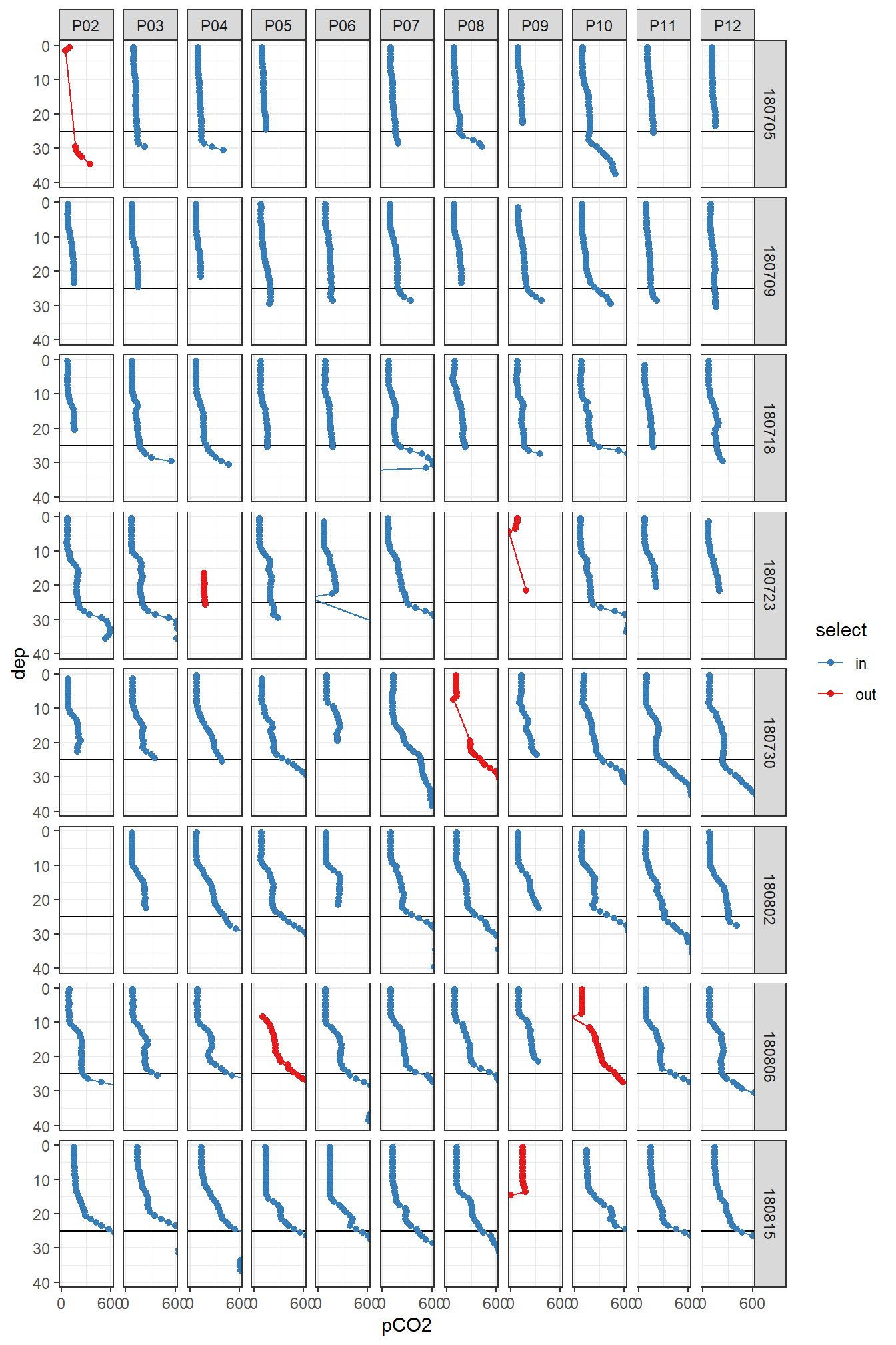
Overview pCO2 profiles at stations (P02-P12) and cruise dates (ID). y-axis restricted to displayed range.
ts_profiles <- ts_profiles %>%
  filter(select == "in") %>%
  select(-select) %>%
  filter(dep < 25)

# assign mean date_time stamp

cruise_dates <- ts_profiles %>%
  group_by(ID) %>%
  summarise(date_time_ID = mean(date_time)) %>%
  ungroup()


# inner_join remove P14 observations lacking date_time_ID
ts_profiles <- inner_join(cruise_dates, ts_profiles)
1.2 Station map
map <- read_csv(here::here("data/Maps","Bathymetry_Gotland_east_small.csv"))

# ggplot()+
#   geom_contour_fill(data=map, aes(x=lon, y=lat, z=-elev), na.fill = TRUE)+
#   coord_quickmap(expand = 0, xlim = c(18.7, 19.9), ylim = c(57.25,57.6))+
#   theme_bw()+
#   theme(legend.position="bottom")

ts_profiles %>%
  group_by(station) %>%
  summarise(lat = mean(lat),
            lon = mean(lon)) %>%
  ungroup() %>%
  ggplot()+
  geom_raster(data=map, aes(lon, lat, fill=-elev))+
  scale_fill_scico(palette = "oslo", na.value = "grey",
                   name="Depth [m]", direction = -1)+
  geom_label(aes(lon, lat, label=station))+
  coord_quickmap(expand = 0, xlim = c(18.7, 19.9), ylim = c(57.25,57.6))+
  theme_bw()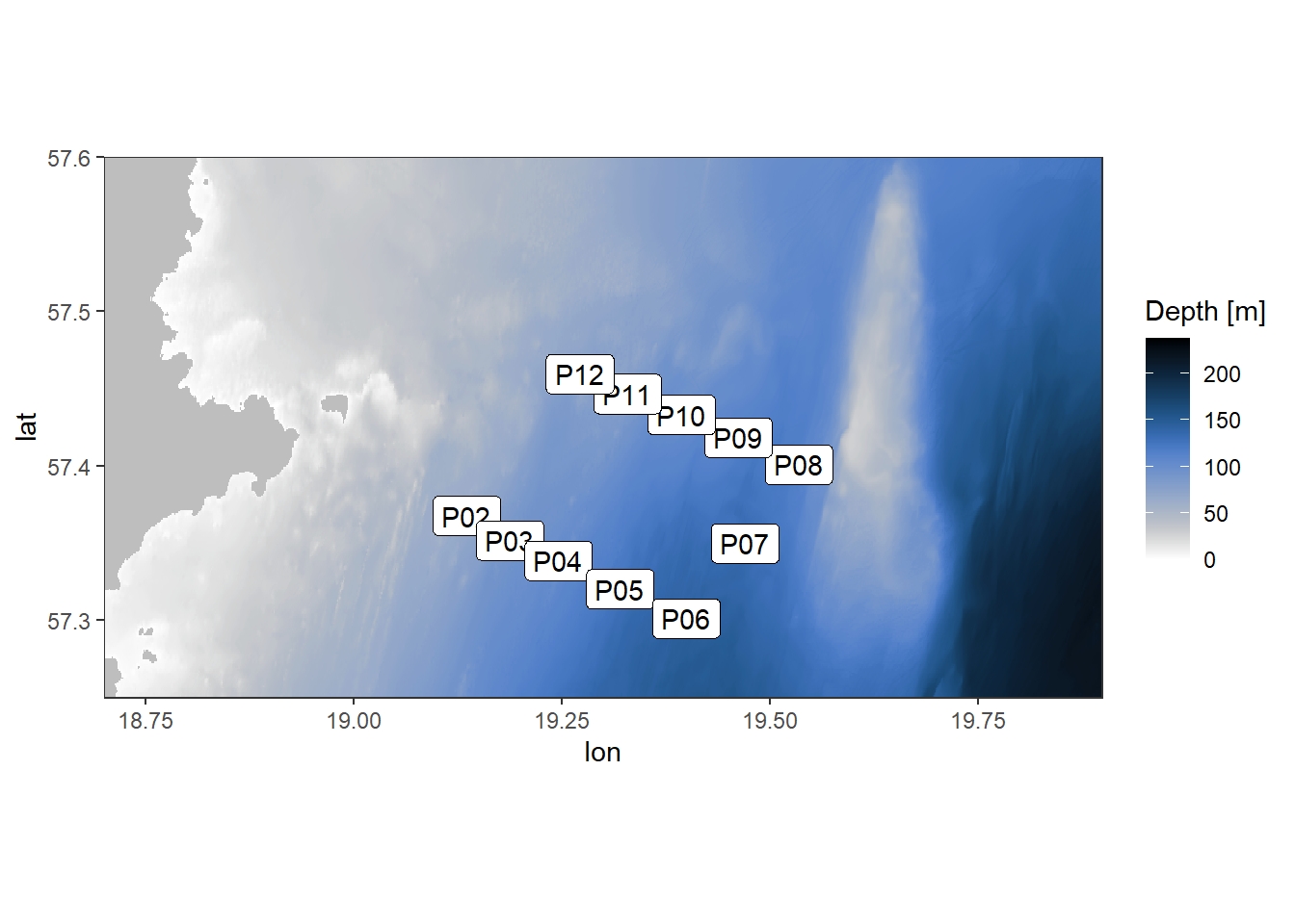
Location of stations sampled between the east coast of Gotland and Gotland deep.
rm(map)1.3 Data coverage
cover <- ts_profiles %>%
  group_by(ID, station) %>%
  summarise(date = mean(date_time),
            date_time_ID = mean(date_time_ID)) %>%
  ungroup()

cover %>%
  ggplot(aes(date, station, fill=ID))+
  geom_vline(aes(xintercept = date_time_ID, col=ID))+
  geom_point(shape=21)+
  scale_color_viridis_d()+
  scale_fill_viridis_d()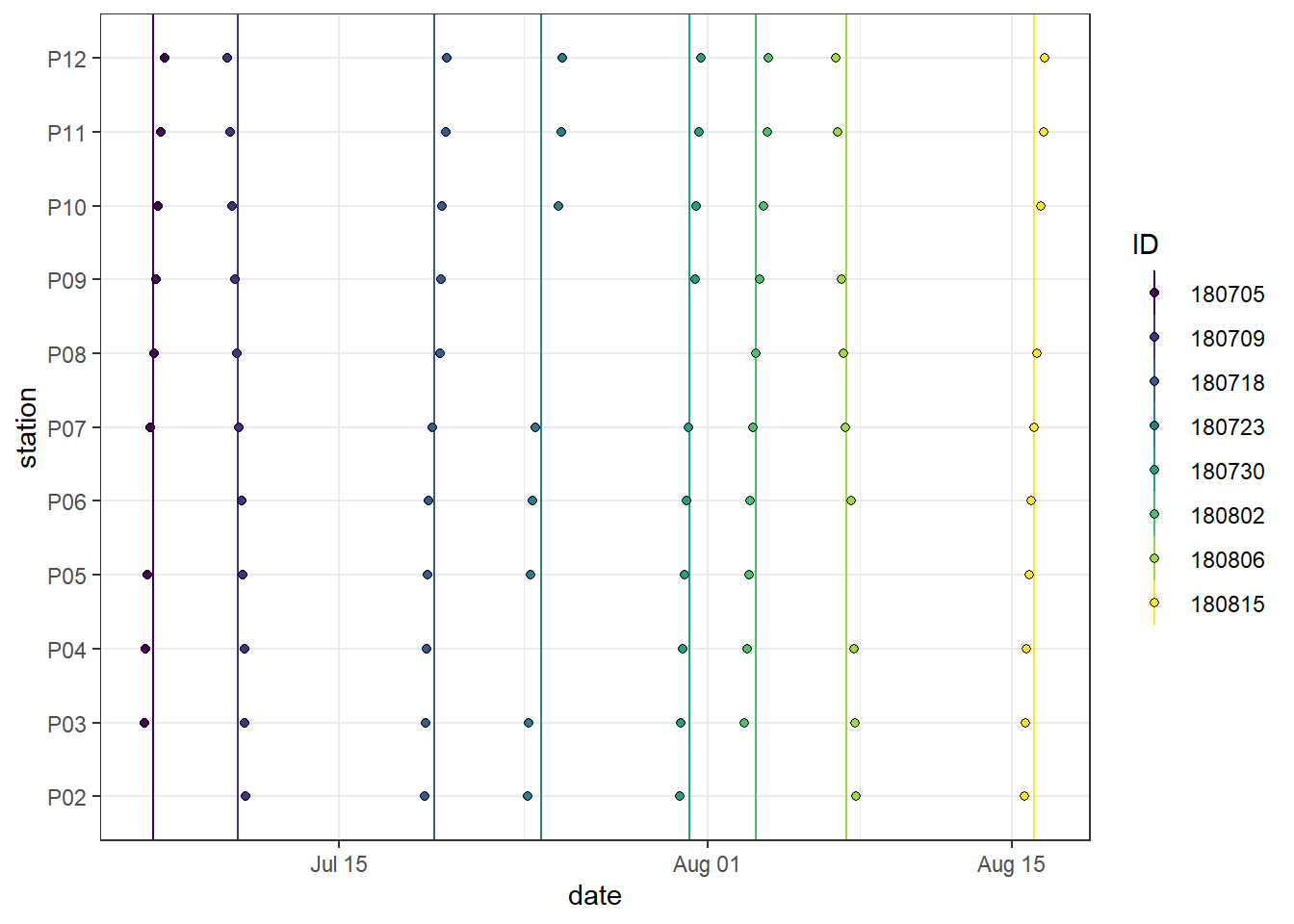
Spatio-temporal data coverage, indicated as station visits over time. ID (color) refers to the starting date of the cruise, except for P14, which was visited twice during each cruise.
rm(cover)2 Bottle CT and AT
At stations P07 and P10 discrete samples for lab measurments of CT and AT were collected. Please note that - in contrast to the pCO2 profiles - samples were taken on June 16, but removed here for harmonization of results.
tb <-
  read_csv(here::here("Data/_summarized_data_files", "Tina_V_Bottle_CO2_lab.csv"),
           col_types = cols(ID = col_character()))

tb <- tb %>%
  filter(station %in% c("P07", "P10")) %>%
  select(-pH_Mosley) %>%
  mutate(CT_AT_ratio = CT/AT)

tb <- inner_join(tb, cruise_dates)
2.1 Vertical profiles
tb_long <- tb %>%
  pivot_longer(4:7, names_to = "var", values_to = "value")

tb_long %>%
  ggplot(aes(value, dep))+
  geom_path(aes(col=ID))+
  geom_point(aes(fill=ID), shape=21)+
  scale_y_reverse()+
  scale_fill_viridis_d()+
  scale_color_viridis_d()+
  facet_grid(station~var, scales = "free_x")+
  theme(legend.position = "bottom")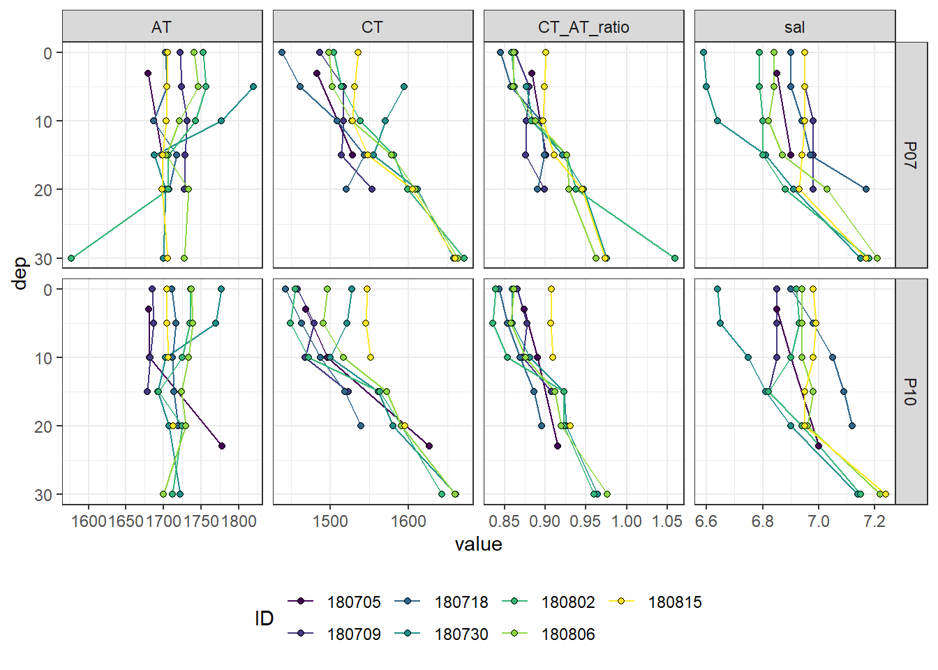
Important notes: - Spatio-temporal variation of AT is small, which jusitfies conversion of pCO2 to CT based on a fixed mean AT - On July 30 we see a drop in surface salinity, associated with a rise in AT, clearly pointing at exchange of water masses, presumably later
2.2 Surface time series
tb_surface <- tb_long %>%
  filter(dep<10) %>%
  group_by(ID, date_time_ID, var, station) %>%
  summarise(value = mean(value, na.rm = TRUE)) %>%
  ungroup()

rm(tb_long)

tb_surface %>%
  ggplot(aes(date_time_ID, value, col=station))+
  #geom_point(aes(lubridate::ymd(ID), value, col=station))+
  geom_point()+
  geom_path()+
  scale_fill_viridis_d()+
  scale_color_brewer(palette = "Set1")+
  facet_grid(var~., scales = "free_y")+
  labs(x="Mean transect date")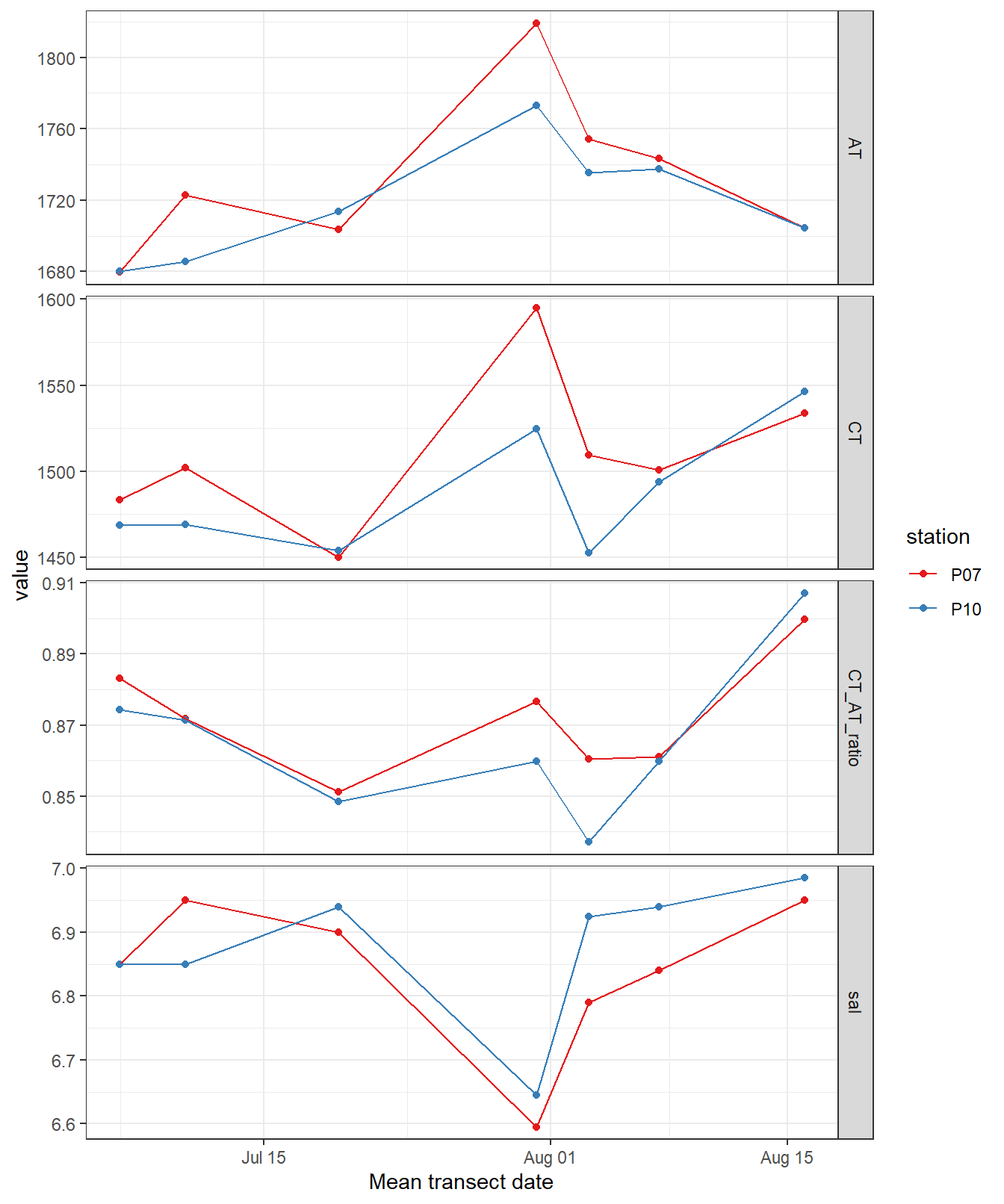
Time series of bottle data. Shown are mean values of samples collected at water depths < 10m (usually collected at 0 and 5 m).
AT_mean <- tb_surface %>%
  filter(var == "AT") %>%
  summarise(AT = mean(value, na.rm = TRUE)) %>%
  pull()

tb_surface %>%
  filter(var == "CT_AT_ratio") %>%
  ggplot(aes(lubridate::ymd(ID), value*AT_mean, col=station))+
  geom_point()+
  geom_path()+
  scale_fill_viridis_d()+
  scale_color_brewer(palette = "Set1")+
  labs(x="Mean transect date", y="CT-AT-ratio * mean AT")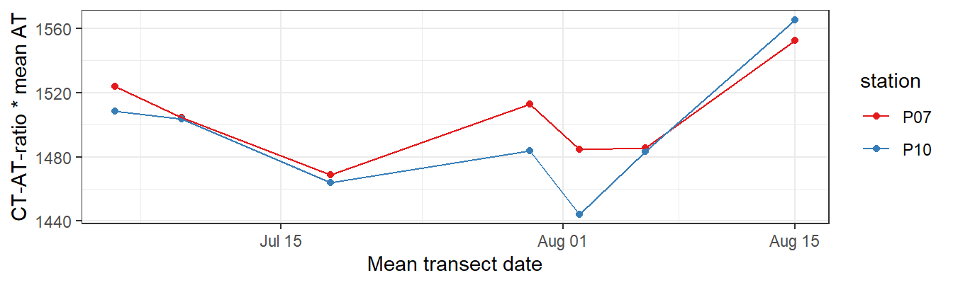
CT timeseries, derived by multiplying the CT-AT-ratio with mean AT
Important notes: - CT drop and temporal patterns observed in the CT/AT time series agrees well with those found in the CT time series derived from pCO2 measurements
2.3 Mean alkalinity
In order to derive CT from measured pCO2 profiles, the mean alkalinity in the upper 20 m and both stations was calculated as:
AT_mean <- tb %>%
  filter(dep <= 20) %>%
  summarise(AT = mean(AT, na.rm = TRUE)) %>%
  pull()

AT_mean
[1] 1717.08Likewise, the mean salinity amounts to:
sal_mean <- tb %>%
  filter(dep <= 20) %>%
  summarise(sal = mean(sal, na.rm = TRUE)) %>%
  pull()

sal_mean
[1] 6.894127bind_cols(start = min(ts$date_time),
end = max(ts$date_time),
AT = AT_mean,
sal = sal_mean) %>%
write_csv(here::here("Data/_summarized_data_files", "tb_fix.csv"))3 CT profiles
3.1 Calculation from pCO2
CT profiles were calculated from sensor pCO2 and T profiles, and constant salinity and alkalinity values. Note that the impact of fixed vs. measured salinity has only a negligible impact on CT profiles.
ts_profiles <- ts_profiles %>%
  drop_na()

ts_profiles <- ts_profiles %>%
  filter(pCO2 > 0)

ts_profiles <- ts_profiles %>%
  mutate(CT = carb(24, var1=pCO2, var2=1720*1e-6,
                   S=sal_mean, T=tem, P=dep/10, k1k2="m10", kf="dg", ks="d",
                   gas="insitu")[,16]*1e6)

rm(sal_mean, AT_mean)

ts_profiles %>%
  write_csv(here::here("Data/_merged_data_files", "ts_profiles_CT.csv"))
3.2 Mean profiles
Mean vertical profiles were calculated for each cruise day (ID).
ts_profiles_ID_mean <- ts_profiles %>%
  select(-c(station,lat, lon, pCO2_raw, date_time)) %>%
  group_by(ID, date_time_ID, dep) %>%
  summarise_all(list(mean), na.rm=TRUE) %>%
  ungroup()

ts_profiles_ID_sd <- ts_profiles %>%
  select(-c(station,lat, lon, pCO2_raw, date_time)) %>%
  group_by(ID, date_time_ID, dep) %>%
  summarise_all(list(sd), na.rm=TRUE) %>%
  ungroup()

ts_profiles_ID_sd_long <- ts_profiles_ID_sd %>%
  pivot_longer(4:7, names_to = "var", values_to = "sd")

ts_profiles_ID_mean_long <- ts_profiles_ID_mean %>%
  pivot_longer(4:7, names_to = "var", values_to = "value")

ts_profiles_ID_long <- inner_join(ts_profiles_ID_mean_long, ts_profiles_ID_sd_long)

rm(ts_profiles_ID_sd_long, ts_profiles_ID_sd, ts_profiles_ID_mean_long, ts_profiles_ID_mean)

ts_profiles_ID_long %>%
  ggplot(aes(value, dep, col=ID))+
  geom_point()+
  geom_path()+
  scale_y_reverse()+
  scale_color_viridis_d()+
  facet_wrap(~var, scales = "free_x")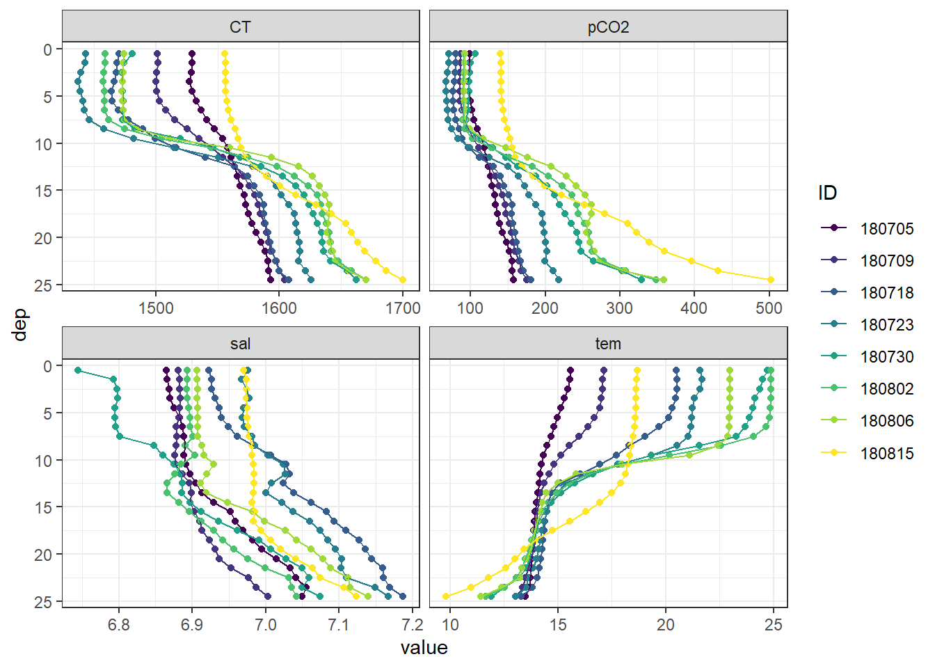
Mean vertical profiles per cruise day across all stations.
all <- ts_profiles_ID_long %>%
  filter(var %in% c("CT", "tem")) %>%
  rename(group = ID)

ts_profiles_ID_long %>%
  filter(var %in% c("CT", "tem")) %>%
  ggplot()+
  geom_path(data=all, aes(value, dep, group=group))+
  geom_ribbon(aes(xmin = value-sd, xmax=value+sd, y=dep, fill=ID), alpha=0.5)+
  geom_path(aes(value, dep, col=ID))+
  scale_y_reverse()+
  scale_color_viridis_d()+
  scale_fill_viridis_d()+
  facet_grid(ID~var, scales = "free_x")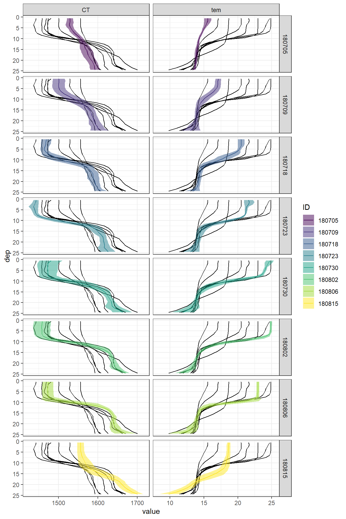
Mean vertical profiles per cruise day across all stations plotted indivdually. Ribbons indicate the standard deviation observed across all profiles at each depth and transect.
rm(all)Important notes:
- the standard deviation of CT in the upper 10m increases on June 30.
3.3 Individual profiles
CT, pCO2, S, and T profiles were plotted individually pdf here and grouped by ID pdf here. The later gives an idea of the differences between stations at one point in time.
pdf(file=here::here("output/Plots/CT_dynamics",
    "ts_profiles_pCO2_tem_sal_CT.pdf"), onefile = TRUE, width = 9, height = 5)

for(i_ID in unique(ts_profiles$ID)){
  for(i_station in unique(ts_profiles$station)){

    if (nrow(ts_profiles %>% filter(ID == i_ID, station == i_station)) > 0){


      # i_ID      <-      unique(ts_profiles$ID)[1]
      # i_station <- unique(ts_profiles$station)[1]

      p_pCO2 <-
        ts_profiles %>%
        arrange(date_time) %>%
        filter(ID == i_ID,
               station == i_station) %>%
        ggplot(aes(pCO2, dep, col="grid_RT"))+
        geom_point(data = ts_profiles_highres %>% arrange(date_time) %>% filter(ID == i_ID, station == i_station),
                   aes(pCO2_raw, dep, col="raw"))+
        geom_point(data = ts_profiles_highres %>% arrange(date_time) %>% filter(ID == i_ID, station == i_station),
                   aes(pCO2, dep, col="raw_RT"))+
        geom_point(aes(pCO2_raw, dep, col="grid"))+
        geom_point()+
        geom_path()+
        scale_y_reverse()+
        scale_color_brewer(palette = "Set1")+
        labs(y="Depth [m]", x="pCO2 [µatm]", title = str_c(i_ID," | ",i_station))+
        coord_cartesian(xlim = c(0,200), ylim = c(30,0))+
        theme_bw()+
        theme(legend.position = "left")

      p_tem <-
        ts_profiles %>%
        arrange(date_time) %>%
        filter(ID == i_ID,
               station == i_station) %>%
        ggplot(aes(tem, dep))+
        geom_point()+
        geom_path()+
        scale_y_reverse()+
        labs(y="Depth [m]", x="Tem [°C]")+
        coord_cartesian(xlim = c(14,26), ylim = c(30,0))+
        theme_bw()

      p_sal <-
        ts_profiles %>%
        arrange(date_time) %>%
        filter(ID == i_ID,
               station == i_station) %>%
        ggplot(aes(sal, dep))+
        geom_point()+
        geom_path()+
        scale_y_reverse()+
        labs(y="Depth [m]", x="Tem [°C]")+
        coord_cartesian(xlim = c(6.5,7.5), ylim = c(30,0))+
        theme_bw()

      p_CT <-
        ts_profiles %>%
        arrange(date_time) %>%
        filter(ID == i_ID,
               station == i_station) %>%
        ggplot(aes(CT, dep))+
        geom_point()+
        geom_path()+
        scale_y_reverse()+
        labs(y="Depth [m]", x="CT* [µmol/kg]")+
        coord_cartesian(xlim = c(1400,1700), ylim = c(30,0))+
        theme_bw()


      print(
            p_pCO2 + p_tem + p_sal + p_CT
            )

      rm(p_pCO2, p_sal, p_tem, p_CT)


    }
  }
}

dev.off()

rm(i_ID, i_station, ts_profiles_highres)
ts_profiles_long <- ts_profiles %>%
select(-c(lat, lon, pCO2_raw)) %>%
pivot_longer(6:9, values_to = "value", names_to = "var")
pdf(file=here::here("output/Plots/CT_dynamics",
"ts_profiles_ID_pCO2_tem_sal_CT.pdf"), onefile = TRUE, width = 9, height = 5)
for(i_ID in unique(ts_profiles$ID)){
#i_ID <- unique(ts_profiles$ID)[1]
sub_ts_profiles_long <- ts_profiles_long %>%
arrange(date_time) %>%
filter(ID == i_ID)
print(
sub_ts_profiles_long %>%
ggplot()+
geom_path(data = ts_profiles_long, aes(value, dep, group=interaction(station, ID)), col="grey")+
geom_path(aes(value, dep, col=station))+
scale_y_reverse()+
labs(y="Depth [m]", title = str_c("ID: ", i_ID))+
theme_bw()+
facet_wrap(~var, scales = "free_x")
)
rm(sub_ts_profiles_long)
}
dev.off()
rm(i_ID, ts_profiles_long)3.4 Profiles of incremental changes
Changes of seawater vars at each depth are calculated from one cruise day to the next and divided by the number of days inbetween.
ts_profiles_ID_long <- ts_profiles_ID_long %>%
    group_by(var, dep) %>%
    arrange(date_time_ID) %>%
    mutate(date_time_ID_diff = as.numeric(date_time_ID - lag(date_time_ID)),
           date_time_ID_ref  = date_time_ID - (date_time_ID - lag(date_time_ID))/2,
           value_diff = value     - lag(value, default = first(value)),
           value_diff_daily = value_diff / date_time_ID_diff,
           value_cum = cumsum(value_diff)) %>%
  ungroup()


ts_profiles_ID_long %>%
  arrange(dep) %>%
  ggplot(aes(value_diff_daily, dep, col=ID))+
  geom_vline(xintercept = 0)+
  geom_point()+
  geom_path()+
  scale_y_reverse()+
  scale_color_viridis_d()+
  facet_wrap(~var, scales = "free_x")+
  labs(x="Change of value inbetween cruises per day")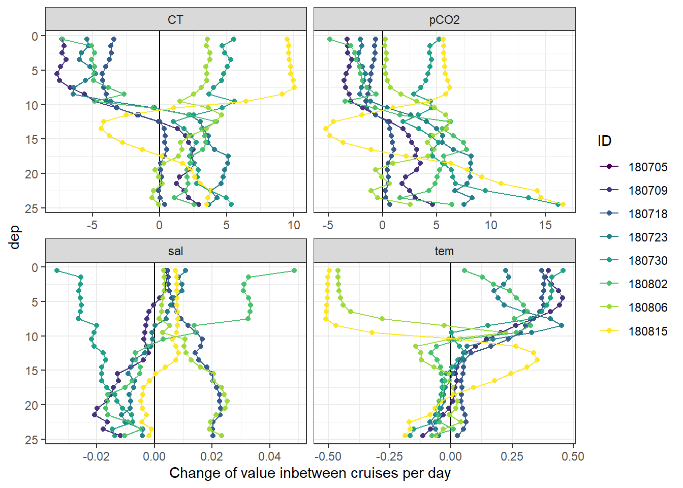
3.5 Profiles of cumulative changes
Cumulative changes of seawater vars were calculated at each depth relative to the first cruise day on July 5.
ts_profiles_ID_long %>%
  arrange(dep) %>%
  ggplot(aes(value_cum, dep, col=ID))+
  geom_vline(xintercept = 0)+
  geom_point()+
  geom_path()+
  scale_y_reverse()+
  scale_color_viridis_d()+
  facet_wrap(~var, scales = "free_x")+
  labs(x="Cumulative change of value")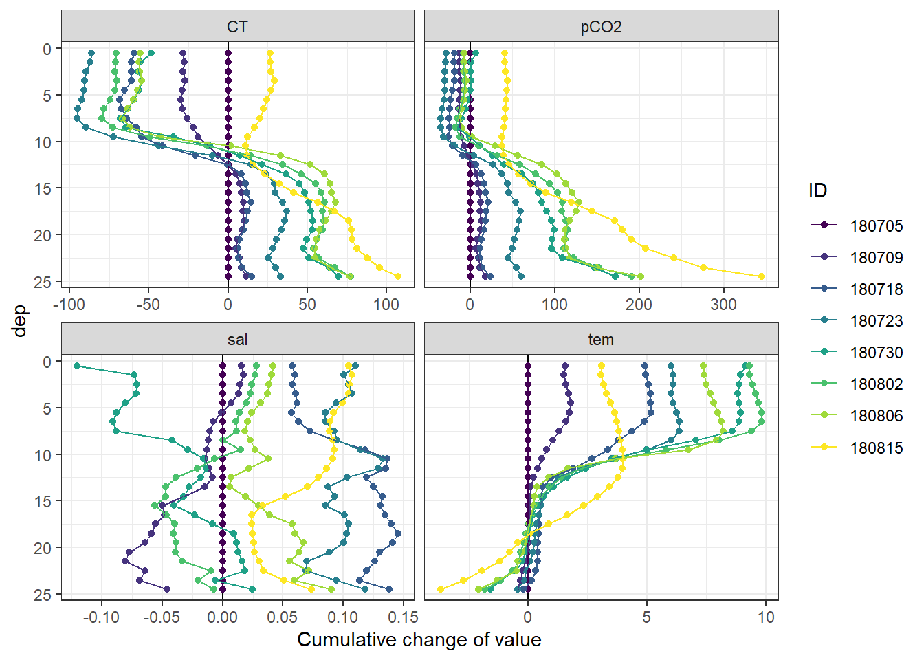
Important notes:
- Salinity in the upper 10m decreases by >0.1 on June 30, and returns to average conditions already on Aug 02.
Cumulative positive and negative changes of seawater vars were calculated separately at each depth relative to the first cruise day on July 5.
ts_profiles_ID_long <- ts_profiles_ID_long %>%
  mutate(sign = if_else(value_diff < 0, "neg", "pos")) %>%
  group_by(var, dep, sign) %>%
  arrange(date_time_ID) %>%
  mutate(value_cum_sign = cumsum(value_diff)) %>%
  ungroup()

ts_profiles_ID_long %>%
  write_csv(here::here("Data/_merged_data_files", "ts_profiles_ID_long_cum.csv"))

ts_profiles_ID_long %>%
  arrange(dep) %>%
  ggplot(aes(value_cum_sign, dep, col=ID))+
  geom_vline(xintercept = 0)+
  geom_point()+
  geom_path()+
  scale_y_reverse()+
  scale_color_viridis_d()+
  scale_fill_viridis_d()+
  facet_wrap(~interaction(sign, var), scales = "free_x", ncol=4)+
  labs(x="Cumulative directional change of value")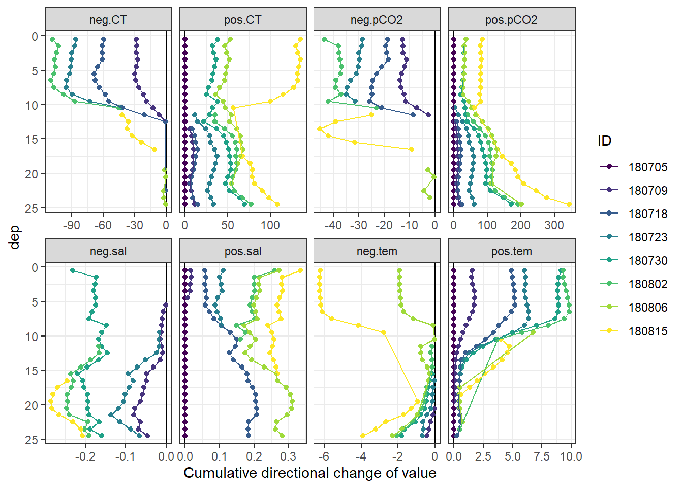
4 Timeseries
4.1 Timeseries depth intervals
Mean seawater parameters were calculated for 5m depth intervals.
ts_profiles_ID_long_grid <- ts_profiles_ID_long %>%
  mutate(dep = cut(dep, seq(0,30,5))) %>%
  group_by(ID, date_time_ID, dep, var)  %>%
  summarise_all(list(mean), na.rm=TRUE)

ts_profiles_ID_long_grid %>%
  ggplot(aes(date_time_ID, value, col=as.factor(dep)))+
  geom_path()+
  #geom_errorbar(aes(date_time_ID, ymax=value+sd, ymin=value-sd, col=as.factor(dep)))+
  geom_point()+
  scale_color_viridis_d(name="Depth [m]")+
  facet_wrap(~var, scales = "free_y", ncol=1)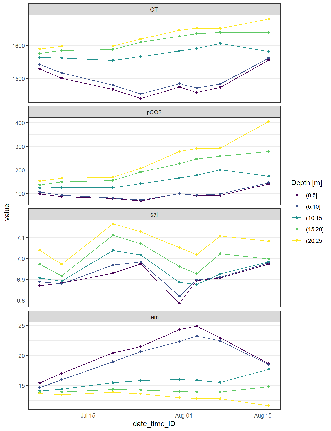
rm(ts_profiles_ID_long_grid)4.2 Hovmoeller plots
4.2.1 Absolute values
bin_CT <- 20

CT_hov <- ts_profiles_ID_long %>%
  filter(var == "CT") %>%
  ggplot()+
  geom_contour_fill(aes(x=date_time_ID, y=dep, z=value),
                    breaks = MakeBreaks(bin_CT),
                    col="black")+
  geom_point(aes(x=date_time_ID, y=c(24.5)), size=3, shape=24, fill="white")+
  scale_fill_viridis_c(breaks = MakeBreaks(bin_CT),
                       guide = "colorstrip",
                       name="CT (µmol/kg)")+
  scale_y_reverse()+
  theme_bw()+
  labs(y="Depth (m)")+
  coord_cartesian(expand = 0)+
  theme(axis.title.x = element_blank(),
        axis.text.x = element_blank())

bin_Tem <- 2

Tem_hov <- ts_profiles_ID_long %>%
  filter(var == "tem") %>%
  ggplot()+
  geom_contour_fill(aes(x=date_time_ID, y=dep, z=value),
                    breaks = MakeBreaks(bin_Tem),
                    col="black")+
  geom_point(aes(x=date_time_ID, y=c(24.5)), size=3, shape=24, fill="white")+
  scale_fill_viridis_c(breaks = MakeBreaks(bin_Tem),
                       guide = "colorstrip",
                       name="Tem (°C)",
                       option = "inferno")+
  scale_y_reverse()+
  theme_bw()+
  labs(x="",y="Depth (m)")+
  coord_cartesian(expand = 0)

CT_hov / Tem_hov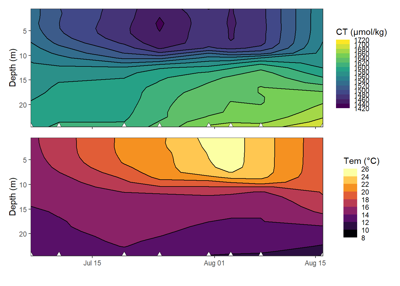
Hovmoeller plots of absolute changes in CT and temperature.
rm(CT_hov, bin_CT, Tem_hov, bin_Tem)4.2.2 Incremental changes
bin_CT <- 2.5

CT_hov <- ts_profiles_ID_long %>%
  filter(var == "CT") %>%
  ggplot()+
  geom_contour_fill(aes(x=date_time_ID_ref, y=dep, z=value_diff_daily),
                    breaks = MakeBreaks(bin_CT),
                    col="black")+
  geom_point(aes(x=date_time_ID, y=c(24.5)), size=3, shape=24, fill="white")+
  scale_fill_divergent(breaks = MakeBreaks(bin_CT),
                       guide = "colorstrip",
                       name="CT (µmol/kg)")+
  scale_y_reverse()+
  theme_bw()+
  labs(y="Depth (m)")+
  coord_cartesian(expand = 0)+
  theme(axis.title.x = element_blank(),
        axis.text.x = element_blank())

bin_Tem <- 0.1

Tem_hov <- ts_profiles_ID_long %>%
  filter(var == "tem") %>%
  ggplot()+
  geom_contour_fill(aes(x=date_time_ID_ref, y=dep, z=value_diff_daily),
                    breaks = MakeBreaks(bin_Tem),
                    col="black")+
  geom_point(aes(x=date_time_ID, y=c(24.5)), size=3, shape=24, fill="white")+
  scale_fill_divergent(breaks = MakeBreaks(bin_Tem),
                       guide = "colorstrip",
                       name="Tem (°C)")+
  scale_y_reverse()+
  theme_bw()+
  labs(x="",y="Depth (m)")+
  coord_cartesian(expand = 0)

CT_hov / Tem_hov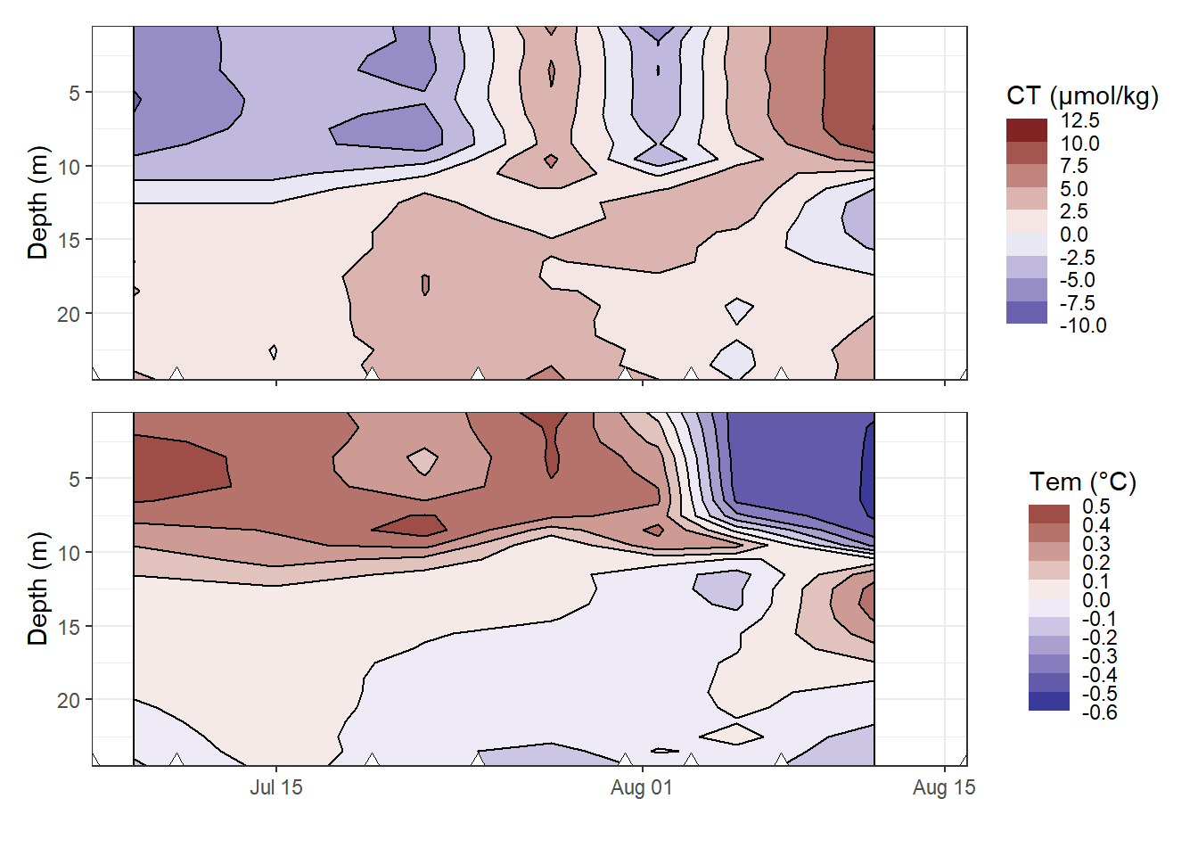
Hovmoeller plots of daily changes in CT and temperature. Note that calculated value of change (in contrast to absolute and cumulative values) are referred to the mean dates inbetween cruise, and are not extrapolated to the full observational period.
rm(CT_hov, bin_CT, Tem_hov, bin_Tem)4.2.3 Cumulative changes
bin_CT <- 20

CT_hov <- ts_profiles_ID_long %>%
  filter(var == "CT") %>%
  ggplot()+
  geom_contour_fill(aes(x=date_time_ID, y=dep, z=value_cum),
                    breaks = MakeBreaks(bin_CT),
                    col="black")+
  geom_point(aes(x=date_time_ID, y=c(24.5)), size=3, shape=24, fill="white")+
  scale_fill_divergent(breaks = MakeBreaks(bin_CT),
                       guide = "colorstrip",
                       name="CT (µmol/kg)")+
  scale_y_reverse()+
  theme_bw()+
  labs(y="Depth (m)")+
  coord_cartesian(expand = 0)+
  theme(axis.title.x = element_blank(),
        axis.text.x = element_blank())

bin_Tem <- 2

Tem_hov <- ts_profiles_ID_long %>%
  filter(var == "tem") %>%
  ggplot()+
  geom_contour_fill(aes(x=date_time_ID, y=dep, z=value_cum),
                    breaks = MakeBreaks(bin_Tem),
                    col="black")+
  geom_point(aes(x=date_time_ID, y=c(24.5)), size=3, shape=24, fill="white")+
  scale_fill_divergent(breaks = MakeBreaks(bin_Tem),
                       guide = "colorstrip",
                       name="Tem (°C)")+
  scale_y_reverse()+
  theme_bw()+
  labs(x="",y="Depth (m)")+
  coord_cartesian(expand = 0)

CT_hov / Tem_hov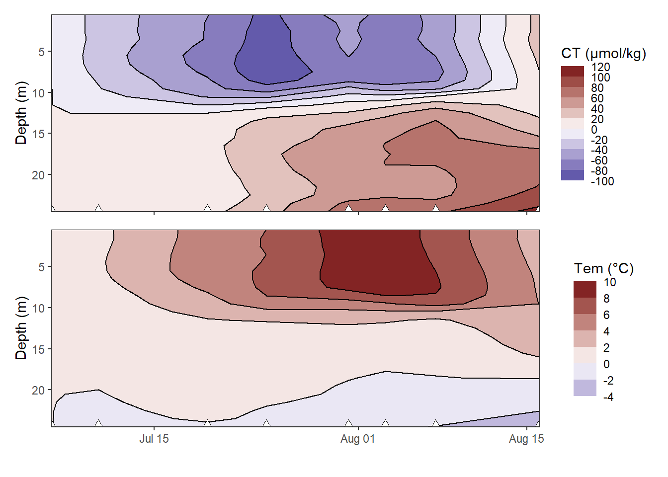
Hovmoeller plots of cumulative changes in CT and temperature.
rm(CT_hov, bin_CT, Tem_hov, bin_Tem)5 Depth-integration of CT changes
A critical first step for the determination of net community production (NCP) is the integration of observed changes in CT over depth to derive iCT. Two approaches were tested:
- Integration of changes in CT over a predefined, fixed water depth
- Integration of changes in CT over a mixed layer depth (MLD)
5.1 Fixed depths
Incremental and cumulative CT changes inbetween cruise dates were integrated across the water colums down to predefined depth limits. This was done separately for observed positive/negative changes in CT, as well as for the total observed changes.
NCP_grid_sign <- ts_profiles_ID_long %>%
  select(ID, date_time_ID, date_time_ID_ref) %>%
  unique() %>%
  expand_grid(sign = c("pos", "neg"))

NCP_grid_total <- ts_profiles_ID_long %>%
  select(ID, date_time_ID, date_time_ID_ref) %>%
  unique() %>%
  expand_grid(sign = c("total"))

# dep_i <- 10
rm(NCP, dep_i)

for (dep_i in seq(5,20,5)) {


NCP_sign_temp <- ts_profiles_ID_long %>%
  filter(var == "CT", dep < dep_i) %>%
  mutate(sign = if_else(ID == "180705" & dep == 0.5, "neg", sign)) %>%
  group_by(ID, date_time_ID, date_time_ID_ref, sign) %>%
  summarise(CT_i_diff = sum(value_diff)/1000) %>%
  ungroup()

NCP_sign_temp <- NCP_sign_temp %>%
  group_by(sign) %>%
  arrange(date_time_ID) %>%
  mutate(CT_i_cum = cumsum(CT_i_diff)) %>%
  ungroup()

NCP_sign_temp <- full_join(NCP_sign_temp, NCP_grid_sign) %>%
  arrange(sign, date_time_ID) %>%
  fill(CT_i_cum)


NCP_total_temp <- ts_profiles_ID_long %>%
  filter(var == "CT", dep < dep_i) %>%
  group_by(ID, date_time_ID, date_time_ID_ref) %>%
  summarise(CT_i_diff = sum(value_diff)/1000) %>%
  ungroup()

NCP_total_temp <- NCP_total_temp %>%
  arrange(date_time_ID) %>%
  mutate(CT_i_cum = cumsum(CT_i_diff)) %>%
  ungroup() %>%
  mutate(sign = "total")

NCP_total_temp <- full_join(NCP_total_temp, NCP_grid_total) %>%
  arrange(sign, date_time_ID) %>%
  fill(CT_i_cum)

NCP_temp <- bind_rows(NCP_sign_temp, NCP_total_temp) %>%
    mutate(dep_i = dep_i)


if (exists("NCP")) {
  NCP <- bind_rows(NCP, NCP_temp)
  } else {NCP <- NCP_temp}

rm(NCP_temp, NCP_sign_temp, NCP_total_temp)

}

rm(NCP_grid_sign, NCP_grid_total)

NCP <- NCP %>%
  mutate(dep_i = as.factor(dep_i))

NCP %>%
  ggplot()+
  geom_point(data = cruise_dates, aes(date_time_ID, 0), shape=21)+
  geom_col(aes(date_time_ID_ref, CT_i_diff, fill=dep_i),
           position = "dodge", alpha=0.3)+
  geom_line(aes(date_time_ID, CT_i_cum, col=dep_i))+
  scale_color_viridis_d(name="Depth limit (m)")+
  scale_fill_viridis_d(name="Depth limit (m)")+
  labs(y="iCT [mol/m2]", x="")+
  facet_grid(sign~., scales = "free_y", space = "free_y")+
  theme_bw()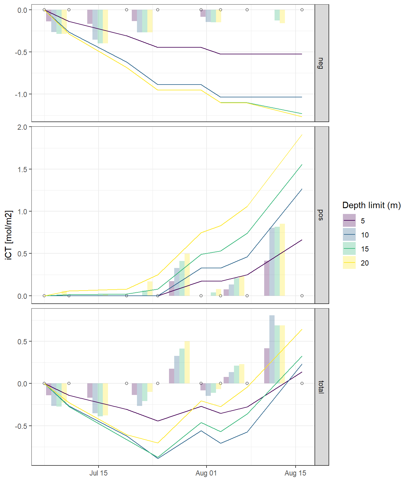
NCP_fixed_dep <- NCP
rm(NCP)
# NCP %>%
#   write_csv(here::here("Data/_merged_data_files", "NCP_dep_limits.csv"))
5.2 MLD approach
As an alternative to fixed depth levels, vertical integration as low as the mixed layer depth was tested.
5.2.1 MLD Calculation
Seawater density Rho was determined from S, T, and p according to TEOS-10.
ts_profiles <- ts_profiles %>%
  mutate(rho = swSigma(salinity = sal, temperature = tem, pressure = dep/10))
5.2.2 Mean hydrographic profiles
ts_profiles_ID_mean_hydro <- ts_profiles %>%
  select(-c(station,lat, lon, pCO2_raw, pCO2, CT, date_time)) %>%
  group_by(ID, date_time_ID, dep) %>%
  summarise_all(list(mean), na.rm=TRUE) %>%
  ungroup()

ts_profiles_ID_sd_hydro <- ts_profiles %>%
  select(-c(station,lat, lon, pCO2_raw, pCO2, CT, date_time)) %>%
  group_by(ID, date_time_ID, dep) %>%
  summarise_all(list(sd), na.rm=TRUE) %>%
  ungroup()


ts_profiles_ID_sd_hydro_long <- ts_profiles_ID_sd_hydro %>%
  pivot_longer(4:6, names_to = "var", values_to = "sd")

ts_profiles_ID_mean_hydro_long <- ts_profiles_ID_mean_hydro %>%
  pivot_longer(4:6, names_to = "var", values_to = "value")

ts_profiles_ID_hydro_long <- inner_join(ts_profiles_ID_mean_hydro_long, ts_profiles_ID_sd_hydro_long)

rm(ts_profiles_ID_sd_hydro_long,
   ts_profiles_ID_sd_hydro,
   ts_profiles_ID_mean_hydro_long)

ts_profiles_ID_hydro_long %>%
  ggplot(aes(value, dep, col=ID))+
  geom_point()+
  geom_path()+
  scale_y_reverse()+
  scale_color_viridis_d()+
  facet_wrap(~var, scales = "free_x")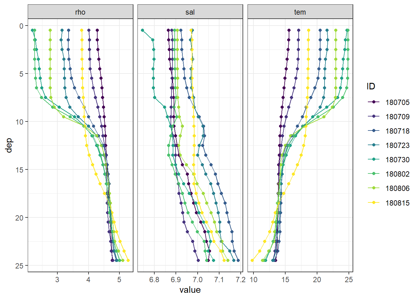
Mean vertical profiles per cruise day across all stations.
5.2.3 MLD timeseries
Mixed layer depth (MLD) was determined based on the difference between density at the surface and at depth, for a range of density criteria
# density criterion

ts_profiles_ID_mean_hydro <- expand_grid(ts_profiles_ID_mean_hydro, rho_lim = c(0.1,0.2,0.5))

MLD <- ts_profiles_ID_mean_hydro  %>%
  arrange(dep) %>%
  group_by(ID, date_time_ID, rho_lim) %>%
  mutate(d_rho = rho - first(rho)) %>%
  filter(d_rho > rho_lim) %>%
  summarise(MLD = min(dep)) %>%
  ungroup()

MLD %>%
  ggplot(aes(date_time_ID, MLD, col=as.factor(rho_lim)))+
  geom_point()+
  geom_path()+
  scale_color_brewer(palette = "Set1", name= "Rho limit")+
  labs(x="")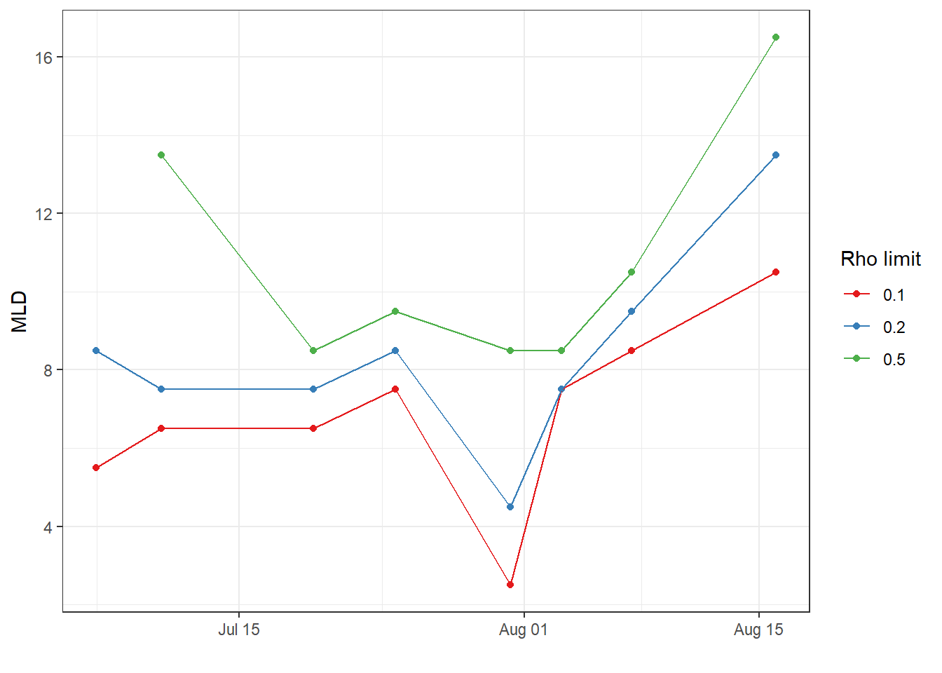
5.2.4 Daily density profiles
ts_profiles_ID_mean_hydro <-
  full_join(ts_profiles_ID_mean_hydro, MLD)

ts_profiles_ID_mean_hydro %>%
  arrange(dep) %>%
  ggplot(aes(rho, dep))+
  geom_hline(aes(yintercept = MLD, col=as.factor(rho_lim)))+
  geom_path()+
  scale_y_reverse()+
  scale_color_discrete(name="Rho lim")+
  facet_wrap(~ID)+
  theme_bw()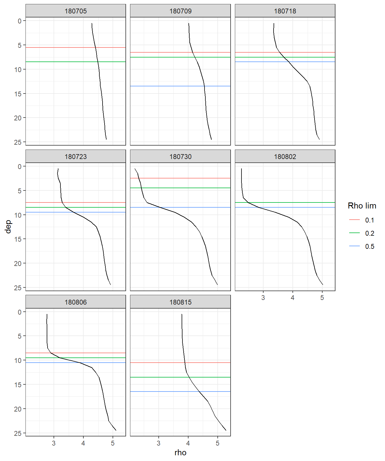
Overview density profiles at stations (P01-P14) and cruise dates (ID). Horizontal lines indicate determined MLD
5.2.5 NCP calculation
# NCP_grid_sign <- ts_profiles_ID_long %>%
#   select(ID, date_time_ID, date_time_ID_ref) %>%
#   unique() %>%
#   expand_grid(sign = c("pos", "neg"))
#
# NCP_grid_total <- ts_profiles_ID_long %>%
#   select(ID, date_time_ID, date_time_ID_ref) %>%
#   unique() %>%
#   expand_grid(sign = c("total"))


NCP <- ts_profiles_ID_long %>%
  filter(var == "CT")

NCP <- full_join(NCP, MLD)

NCP <- NCP %>%
  filter(dep <= MLD)

NCP <- NCP %>%
  group_by(ID, date_time_ID, date_time_ID_ref, rho_lim) %>%
  summarise(CT_i_diff = sum(value_diff)/1000) %>%
  ungroup()

NCP <- NCP %>%
  group_by(rho_lim) %>%
  arrange(date_time_ID) %>%
  mutate(CT_i_cum = cumsum(CT_i_diff)) %>%
  ungroup()

# NCP_total_temp <- full_join(NCP_total_temp, NCP_grid_total) %>%
#   arrange(sign, date_time_ID) %>%
#   fill(CT_i_cum)

NCP <- NCP %>%
  mutate(rho_lim = as.factor(rho_lim))

NCP %>%
  ggplot()+
  geom_point(data = cruise_dates, aes(date_time_ID, 0), shape=21)+
  geom_col(aes(date_time_ID_ref, CT_i_diff, fill=rho_lim),
           position = "dodge", alpha=0.3)+
  geom_line(aes(date_time_ID, CT_i_cum, col=rho_lim))+
  scale_color_viridis_d(name="Rho limit")+
  scale_fill_viridis_d(name="Rho limit")+
  labs(y="iCT [mol/m2]", x="")+
  #facet_grid(sign~., scales = "free_y", space = "free_y")+
  theme_bw()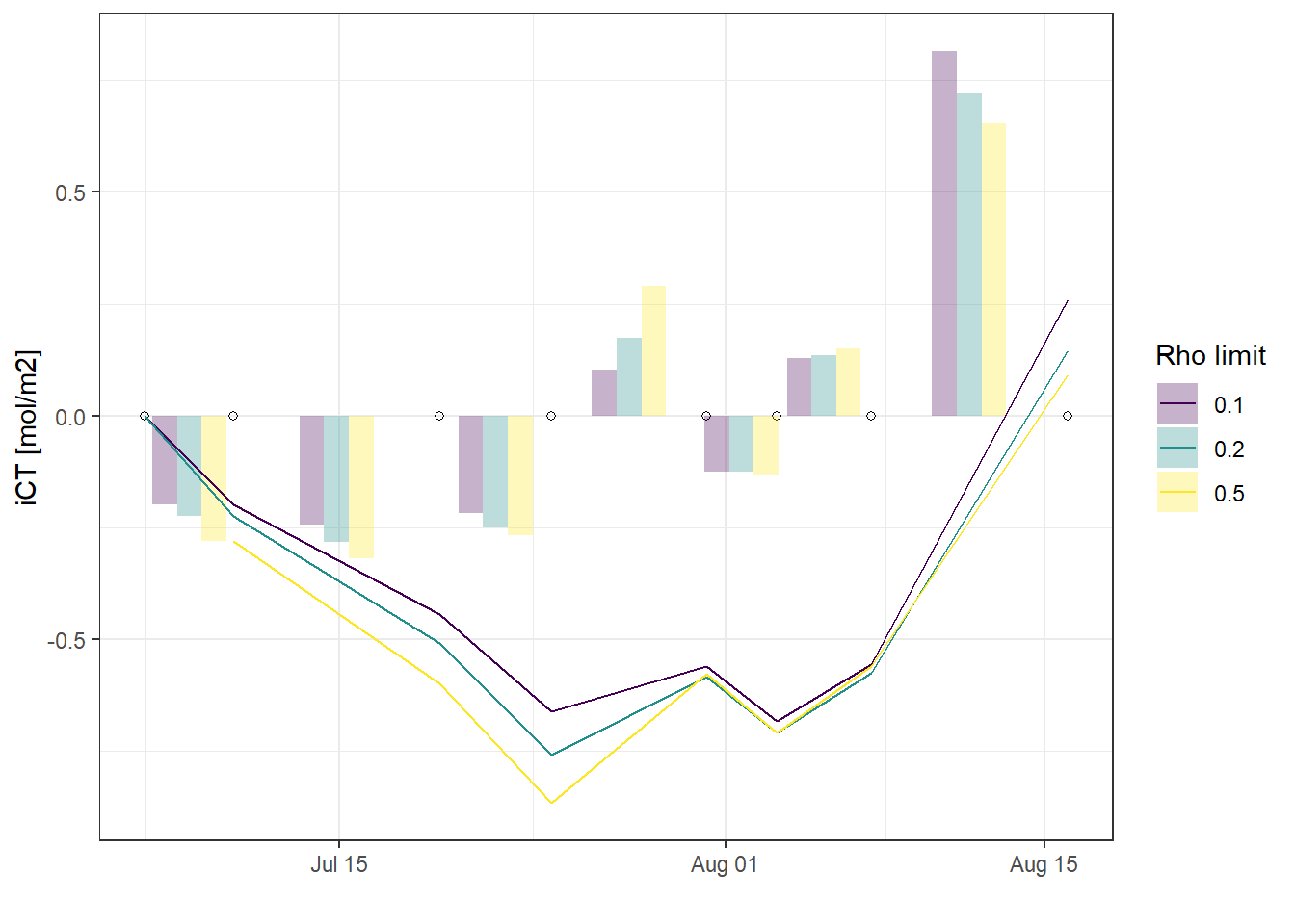
NCP_MLD <- NCP
rm(NCP)

# NCP %>%
#   write_csv(here::here("Data/_merged_data_files", "NCP_dep_limits.csv"))
5.3 Comparison of approaches
NCP <- full_join(NCP_fixed_dep, NCP_MLD)

NCP <- NCP %>%
  mutate(group = paste(as.character(sign), as.character(dep_i), as.character(rho_lim)))

NCP %>%
  arrange(date_time_ID) %>%
  ggplot()+
  geom_hline(yintercept = 0)+
  geom_point(data = cruise_dates, aes(date_time_ID, 0), shape=21)+
  geom_line(aes(date_time_ID, CT_i_cum,
                group=group), col="grey")+
  geom_line(data = NCP_fixed_dep %>% filter(dep_i==10, sign=="total"),
            aes(date_time_ID, CT_i_cum, col="10m - total"))+
  geom_line(data = NCP_MLD %>% filter(rho_lim == 0.1),
            aes(date_time_ID, CT_i_cum, col="MLD - 0.1"))+
  scale_color_brewer(palette = "Set1", name="")+
  labs(y="iCT [mol/m2]", x="")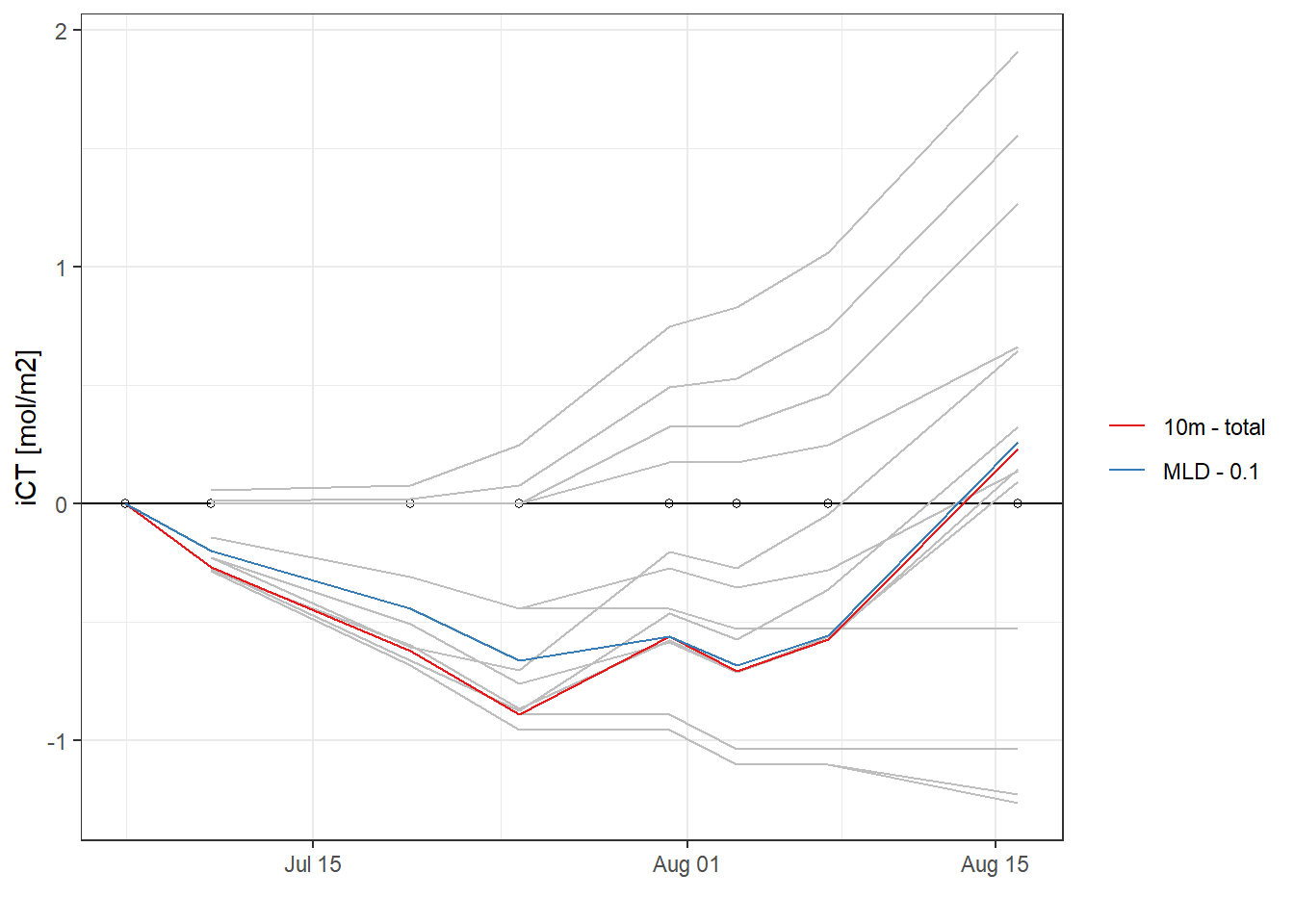
rm(NCP, NCP_fixed_dep, NCP_MLD)5.4 Depth of first production pulse
Approach: Determine the depth across which most of the NCP signal was observed after the initial production pulse on July 23. Thereafter, restrict calcualtion of cummulative CT changes to that depth.
NCP <- ts_profiles_ID_long %>%
  filter(ID == 180723,
         var == "CT")

NCP %>%
  arrange(dep) %>%
  ggplot(aes(value_cum, dep, col="total"))+
  geom_vline(xintercept = 0)+
  geom_path(aes(value_cum_sign, dep, col="directional"))+
  geom_point(aes(value_cum_sign, dep, col="directional"))+
  geom_point()+
  geom_path()+
  scale_y_reverse()+
  scale_color_brewer(palette = "Set1", name="estimate")+
  labs(x="Cumulative change of CT on July 23 (180723)")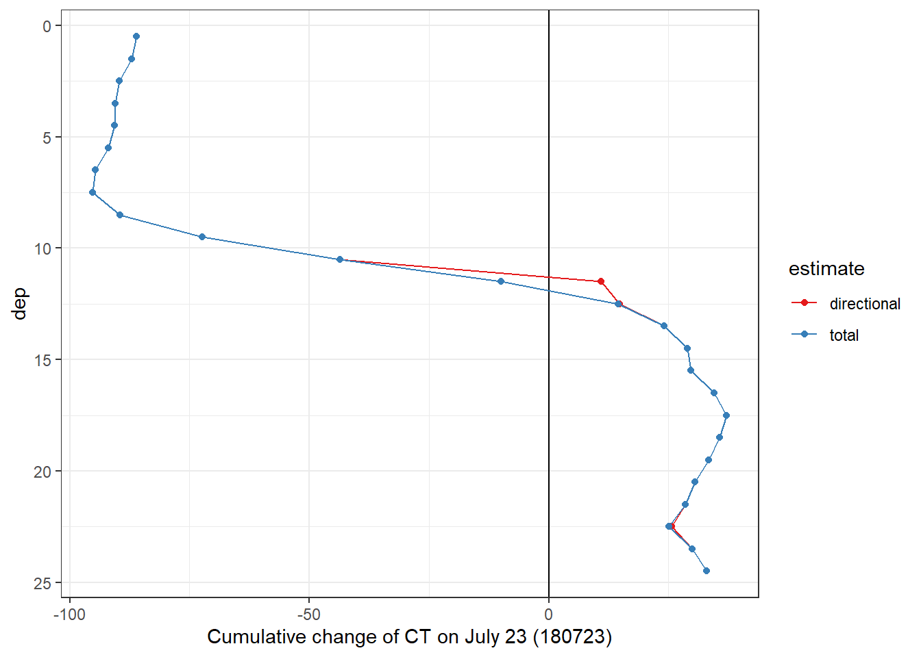
NCP_dep <- NCP %>%
  select(dep, value_cum) %>%
  filter(value_cum < 0) %>%
  arrange(dep) %>%
  mutate(value_cum_i = sum(value_cum),
         value_cum_dep = cumsum(value_cum),
         value_cum_i_rel = value_cum_dep/value_cum_i*100)

NCP_dep %>%
  ggplot(aes(dep, value_cum_i_rel))+
  geom_hline(yintercept = 90, col="red")+
  geom_point()+
  geom_line()+
  labs(x="Depth (m)", y = "Relative contribution to NCP on July 23")+
  ylim(0,100)+
  theme_bw()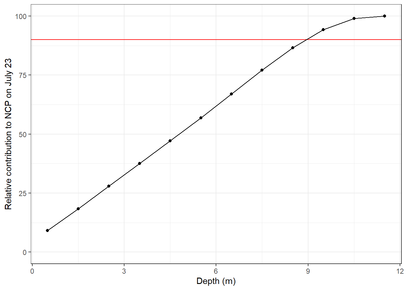
rm(NCP, NCP_dep)90% of the cumulative NCP observed until July 23 is observed and homogeniouly spread across the upper ten metres of the water column. The intial idea to restrict ongoing CT changes after July 23 to the depth were most of the NCP signal was located is stopped here, as it would lead to the exact same result as the intergration over the upper 10 m of the water column executed above.
5.5 Air-Sea CO2 flux
6 Old schript parts
NCP <- ts_profiles_ID_long %>%
  filter(var == "CT") %>%
  mutate(dep = cut(dep, seq(0,30,5))) %>%
  group_by(ID, date_time_ID, dep, sign) %>%
  summarise(dCT = sum(value_diff)/1000) %>%
  ungroup()

NCP <- NCP %>%
  group_by(sign, dep) %>%
  arrange(date_time_ID) %>%
  mutate(dCT_cum = cumsum(dCT)) %>%
  ungroup()

NCP %>%
  write_csv(here::here("Data/_merged_data_files", "BloomSail_CTD_HydroC_CT_cumulative_timeseries.csv"))


NCP_grid <- expand_grid(
  unique(NCP$date_time_ID),
  unique(NCP$dep),
  unique(NCP$sign)
)

NCP_grid <- NCP_grid %>%
  set_names(c("date_time_ID","dep", "sign"))

NCP <- full_join(NCP, NCP_grid)

rm(NCP_grid)

NCP <- NCP %>%
  arrange(sign, dep, date_time_ID) %>%
  group_by(sign, dep) %>%
  fill(dCT_cum) %>%
  ungroup() %>%
  mutate(dCT_cum = if_else(is.na(dCT_cum), 0, dCT_cum))
p_iNCP <- NCP %>%
ggplot(aes(date_time_ID, dCT, fill=dep))+
geom_hline(yintercept = 0)+
geom_bar(stat="identity", col="black")+
scale_fill_viridis_d()+
scale_y_continuous(breaks = seq(-100, 100, 0.2))+
facet_grid(rev(sign)~., scales = "free_y", space = "free_y")+
theme(strip.background = element_blank(),
strip.text = element_blank())+
labs(y="integrated, directional CT changes [mol/m2]", x="date")
p_iNCPcum <- NCP %>%
ggplot(aes(date_time_ID, dCT_cum, fill=dep))+
geom_hline(yintercept = 0)+
geom_area(col="black")+
scale_fill_viridis_d()+
scale_y_continuous(breaks = seq(-100, 100, 0.2))+
facet_grid(rev(sign)~., scales = "free_y", space = "free_y")+
theme(strip.background = element_blank(),
strip.text = element_blank())+
labs(y="integrated, cumulative, directional CT changes [mol/m2]", x="date")
(p_iNCP / p_iNCPcum)+
plot_layout(guides = 'collect')
rm(p_iNCP, p_iNCPcum)7 Nomenclature of objectes
Should be identical for stored files and objectes in R environment
- source
- ts: tina 5 sensor
- tb: tina 5 bottle
- fm: finnmaid
- og: ostergarnsholm tower
- mp: bathymetric map
- subsetting and modification levels
- profiles vs surface: operation mode tina 5
- ID: mean values for cruise (reduced temporal resolution)
- daily: daily mean values
- long: data stored in long format (all observations in only 2 columns “var” and “value”)
- fix: constant, unique values such as long-term means, starting dates, etc
- NCP: includes cumulative numbers as NCP estimates
- CT_tem: data subset to analyse changes of CT with tem
- 3d vs 2d: surface vs depth resolved GETM data
8 Nomenclature of variables
- Descriptive variables
- date
- date_time
- date_time_ID: mean date of cruise
- date_time_ID_diff: time differences in between cruises
- date_time_ID_ref: mean date in between cruises corresponding to observed incremental changes
- station
- ID: character identifying starting date of cruise as YYMMDD
- dep: 1m depth intervals
- lat
- lon
- Observed variables: column names, or identifier in column “var” for long-format tables
- pCO2
- sal
- tem
- CT
- U10: wind speed at 10m
- mld: mixed or mixing layer depth
- Variable name extension
- mean
- sd
- min
- max
- int: interpolated value
- grid: value gridded to a coarser resolution
- diff: difference to previous value
- diff_daily: difference to previous value divided by number of days
- i: intergrated over depth
- cum: cumulative value over time
- sign: identifier for pos. or neg. differences
- p_XXX: ggplot object
9 NCP estimation
Possible approaches
- cumulative negative changes of CT + positive changes in range where negative changes occured
- cumulative changes of CT above MLD
- cumulative positive changes of CT above MLD
10 Open tasks / questions
- clean and harmonize chunk labeling (label: plot, 1 plot per chunk, etc)
- included removed stations in map and coverage plot
- Significance of changes in AT for calculated CT changes
- Harmonize selection of profiles for tau optimization and BGC interpretation (how many missing discrete depth intervals are allowed?)
sessionInfo()R version 3.5.0 (2018-04-23)
Platform: x86_64-w64-mingw32/x64 (64-bit)
Running under: Windows 10 x64 (build 18363)
Matrix products: default
locale:
[1] LC_COLLATE=English_United States.1252
[2] LC_CTYPE=English_United States.1252
[3] LC_MONETARY=English_United States.1252
[4] LC_NUMERIC=C
[5] LC_TIME=English_United States.1252
attached base packages:
[1] stats graphics grDevices utils datasets methods base
other attached packages:
[1] scico_1.1.0 metR_0.5.0 seacarb_3.2.12 oce_1.2-0
[5] gsw_1.0-5 testthat_2.3.1 patchwork_1.0.0 forcats_0.4.0
[9] stringr_1.4.0 dplyr_0.8.3 purrr_0.3.3 readr_1.3.1
[13] tidyr_1.0.0 tibble_2.1.3 ggplot2_3.3.0 tidyverse_1.3.0
loaded via a namespace (and not attached):
[1] nlme_3.1-137 bitops_1.0-6 fs_1.3.1
[4] lubridate_1.7.4 RColorBrewer_1.1-2 httr_1.4.1
[7] rprojroot_1.3-2 tools_3.5.0 backports_1.1.5
[10] R6_2.4.0 DBI_1.0.0 colorspace_1.4-1
[13] withr_2.1.2 sp_1.3-2 tidyselect_0.2.5
[16] gridExtra_2.3 compiler_3.5.0 git2r_0.26.1
[19] cli_1.1.0 rvest_0.3.5 xml2_1.2.2
[22] labeling_0.3 scales_1.0.0 checkmate_1.9.4
[25] digest_0.6.22 foreign_0.8-70 rmarkdown_2.0
[28] pkgconfig_2.0.3 htmltools_0.4.0 dbplyr_1.4.2
[31] highr_0.8 maps_3.3.0 rlang_0.4.5
[34] readxl_1.3.1 rstudioapi_0.10 generics_0.0.2
[37] jsonlite_1.6 RCurl_1.95-4.12 magrittr_1.5
[40] Formula_1.2-3 dotCall64_1.0-0 Matrix_1.2-14
[43] Rcpp_1.0.2 munsell_0.5.0 lifecycle_0.1.0
[46] stringi_1.4.3 yaml_2.2.0 plyr_1.8.4
[49] grid_3.5.0 maptools_0.9-8 formula.tools_1.7.1
[52] promises_1.1.0 crayon_1.3.4 lattice_0.20-35
[55] haven_2.2.0 hms_0.5.2 zeallot_0.1.0
[58] knitr_1.26 pillar_1.4.2 reprex_0.3.0
[61] glue_1.3.1 evaluate_0.14 data.table_1.12.6
[64] modelr_0.1.5 operator.tools_1.6.3 vctrs_0.2.0
[67] spam_2.3-0.2 httpuv_1.5.2 cellranger_1.1.0
[70] gtable_0.3.0 assertthat_0.2.1 xfun_0.10
[73] broom_0.5.3 later_1.0.0 viridisLite_0.3.0
[76] memoise_1.1.0 fields_9.9 workflowr_1.6.0
[79] ellipsis_0.3.0 here_0.1