MLD
Jens Daniel Müller
28 April, 2020
Last updated: 2020-04-28
Checks: 7 0
Knit directory: BloomSail/
This reproducible R Markdown analysis was created with workflowr (version 1.6.1). The Checks tab describes the reproducibility checks that were applied when the results were created. The Past versions tab lists the development history.
Great! Since the R Markdown file has been committed to the Git repository, you know the exact version of the code that produced these results.
Great job! The global environment was empty. Objects defined in the global environment can affect the analysis in your R Markdown file in unknown ways. For reproduciblity it’s best to always run the code in an empty environment.
The command set.seed(20191021) was run prior to running the code in the R Markdown file. Setting a seed ensures that any results that rely on randomness, e.g. subsampling or permutations, are reproducible.
Great job! Recording the operating system, R version, and package versions is critical for reproducibility.
Nice! There were no cached chunks for this analysis, so you can be confident that you successfully produced the results during this run.
Great job! Using relative paths to the files within your workflowr project makes it easier to run your code on other machines.
Great! You are using Git for version control. Tracking code development and connecting the code version to the results is critical for reproducibility.
The results in this page were generated with repository version 058c709. See the Past versions tab to see a history of the changes made to the R Markdown and HTML files.
Note that you need to be careful to ensure that all relevant files for the analysis have been committed to Git prior to generating the results (you can use wflow_publish or wflow_git_commit). workflowr only checks the R Markdown file, but you know if there are other scripts or data files that it depends on. Below is the status of the Git repository when the results were generated:
Ignored files:
    Ignored:    .Rhistory
    Ignored:    .Rproj.user/
    Ignored:    data/Finnmaid_2018/
    Ignored:    data/GETM/
    Ignored:    data/Maps/
    Ignored:    data/Ostergarnsholm/
    Ignored:    data/TinaV/
    Ignored:    data/_merged_data_files/
    Ignored:    data/_summarized_data_files/
    Ignored:    output/Plots/Figures_publication/.tmp.drivedownload/
    Ignored:    output/Plots/Figures_publication/Appendix/
Note that any generated files, e.g. HTML, png, CSS, etc., are not included in this status report because it is ok for generated content to have uncommitted changes.
These are the previous versions of the repository in which changes were made to the R Markdown (analysis/BloomSail_surface.Rmd) and HTML (docs/BloomSail_surface.html) files. If you’ve configured a remote Git repository (see ?wflow_git_remote), click on the hyperlinks in the table below to view the files as they were in that past version.
| File | Version | Author | Date | Message |
|---|---|---|---|---|
| html | 66b4ba3 | jens-daniel-mueller | 2020-04-28 | Build site. |
| Rmd | 4f17cbb | jens-daniel-mueller | 2020-04-28 | zeff for Finnmaid data |
| html | c7eb7dd | jens-daniel-mueller | 2020-04-27 | Build site. |
| Rmd | b12f534 | jens-daniel-mueller | 2020-04-27 | Comparison of iCT approaches |
| html | d7bdade | jens-daniel-mueller | 2020-04-27 | Build site. |
| Rmd | 9f738eb | jens-daniel-mueller | 2020-04-27 | removed zeff from MLD section |
| html | 7d38881 | jens-daniel-mueller | 2020-04-27 | Build site. |
| Rmd | 14c8848 | jens-daniel-mueller | 2020-04-27 | tem CT penetration depth |
| html | 6fdf22f | jens-daniel-mueller | 2020-04-27 | Build site. |
| Rmd | f73f073 | jens-daniel-mueller | 2020-04-27 | removed Date-ID column causing error |
| html | 472c2b4 | jens-daniel-mueller | 2020-04-21 | Build site. |
| Rmd | a82b4fe | jens-daniel-mueller | 2020-04-21 | try rebuild all html |
| html | f8fcf50 | jens-daniel-mueller | 2020-04-19 | created pub figures for time series |
| html | dc275fe | jens-daniel-mueller | 2020-04-14 | Build site. |
| Rmd | 2e7d3a5 | jens-daniel-mueller | 2020-04-14 | temperature penetration depth eval TRUE |
| html | 87658c3 | jens-daniel-mueller | 2020-04-14 | Build site. |
| Rmd | 5c96a65 | jens-daniel-mueller | 2020-04-14 | temperature penetration depth |
| html | f4a27b8 | jens-daniel-mueller | 2020-04-01 | Build site. |
| Rmd | b1613b7 | jens-daniel-mueller | 2020-04-01 | re-calculated MLD, renamed objects and structured site |
| html | 1465fb5 | jens-daniel-mueller | 2020-03-31 | Build site. |
| Rmd | 2ebefdf | jens-daniel-mueller | 2020-03-31 | Finalized Baltic surface reconstruction |
| html | 6302994 | jens-daniel-mueller | 2020-03-31 | Build site. |
| Rmd | 50ab313 | jens-daniel-mueller | 2020-03-31 | implemented temperature reconstruction |
| html | ce0f1cf | jens-daniel-mueller | 2020-03-30 | Build site. |
| Rmd | c2d1b89 | jens-daniel-mueller | 2020-03-30 | activated chunks |
| html | a6c4c22 | jens-daniel-mueller | 2020-03-30 | Build site. |
| Rmd | d8120b3 | jens-daniel-mueller | 2020-03-30 | reconstruction BloomSail surface started, merging MLD and DT approach |
| Rmd | a135643 | jens-daniel-mueller | 2020-03-20 | renamed |
| html | a025f62 | jens-daniel-mueller | 2020-03-20 | Build site. |
| Rmd | 39c69a3 | jens-daniel-mueller | 2020-03-20 | knit BloomSail surface |
library(tidyverse)
library(seacarb)
library(oce)
library(marelac)
library(patchwork)
library(metR)
library(lubridate)
1 Approach
In order to test how (and how well) the depth-integrated CT estimates can be reproduced if only surface CO2 data were available, the BloomSail observations were restricted to those made in surface water and following reconstruction approaches were tested:
- Mixed layer depth: Integration of surface observation across the MLD, assuming homogenious vertical patterns
- CT profile reconstruction: Vertical reconstruction of incremental CT changes based on profiles of incremental changes in temperature
- Temperature penetration depth: Integration of surface observation across the temperature penetration depth, assuming similar vertical extension as for CT drawdown.
Note: The reconstruction of CT profiles and the integration across the temperature penetration depth should produce very similar results. However, the latter avoids to create misinterpretable information about the vertical distribution of CT.
2 Data base
1m gridded, downcast profiles were used. CO2 data other than 3.5 m water depth were removed.
3 MLD approach
MLD calculation was previously described in the CT dynamics chapter.
3.1 Read data
ts_profiles_ID <-
  read_csv(here::here("Data/_merged_data_files", "ts_profiles_ID_long_cum_MLD.csv"))

ts_profiles_ID <- ts_profiles_ID %>%
  select(ID, date_time_ID, dep, CT = value, CT_diff = value_diff, CT_cum = value_cum, sign, rho_lim, MLD)

ts_profiles_ID <- ts_profiles_ID %>%
  mutate(rho_lim = as.factor(rho_lim))
ts_profiles_ID <- ts_profiles_ID %>%
mutate(CT = if_else(dep == 3.5, CT, NaN),
rho_lim = as.factor(rho_lim))3.2 Timeseries
ts_profiles_ID %>%
  ggplot()+
  geom_hline(yintercept = 0)+
  geom_line(aes(date_time_ID, MLD, col=rho_lim, linetype="MLD"))+
  scale_y_reverse()+
  scale_color_viridis_d(name="Rho limit")+
  scale_linetype(name="Estimate")+
  labs(y="Depth (m)")+
  theme(axis.title.x = element_blank())
3.3 iCT calculation
Integrated CT depletion was calculated as the product of observed incremental CT changes in surface waters and the respective mixed layer depth.
ts_profiles_ID_surface <- ts_profiles_ID %>%
  filter(dep==3.5) %>%
  group_by(rho_lim) %>%
  arrange(date_time_ID) %>%
  mutate(iCT_diff = CT_diff * MLD / 1000,
         iCT_cum = cumsum(replace_na(iCT_diff, 0))) %>%
  ungroup()
3.4 Incremental and cumulative timeseries
Total incremental and cumulative CT changes inbetween cruise dates were calculated.
p_iCT <- ts_profiles_ID_surface %>%
  ggplot(aes(date_time_ID, iCT_diff, fill= rho_lim))+
  geom_hline(yintercept = 0)+
  geom_col(col="black", position = "dodge")+
  scale_y_continuous(breaks = seq(-100, 100, 0.2))+
  scale_fill_viridis_d()+
  labs(y="integrated CT changes [mol/m2]")+
  theme(axis.title.x = element_blank())

p_iCT_cum <- ts_profiles_ID_surface %>%
  ggplot(aes(date_time_ID,  iCT_cum,
             col=rho_lim))+
  geom_line()+
  geom_hline(yintercept = 0)+
  scale_color_viridis_d()+
  scale_y_continuous(breaks = seq(-100, 100, 0.2))+
  theme(strip.background = element_blank(),
        strip.text = element_blank())+
  labs(y="integrated, cumulative CT changes [mol/m2]", x="date")


(p_iCT / p_iCT_cum)+
  plot_layout(guides = 'collect')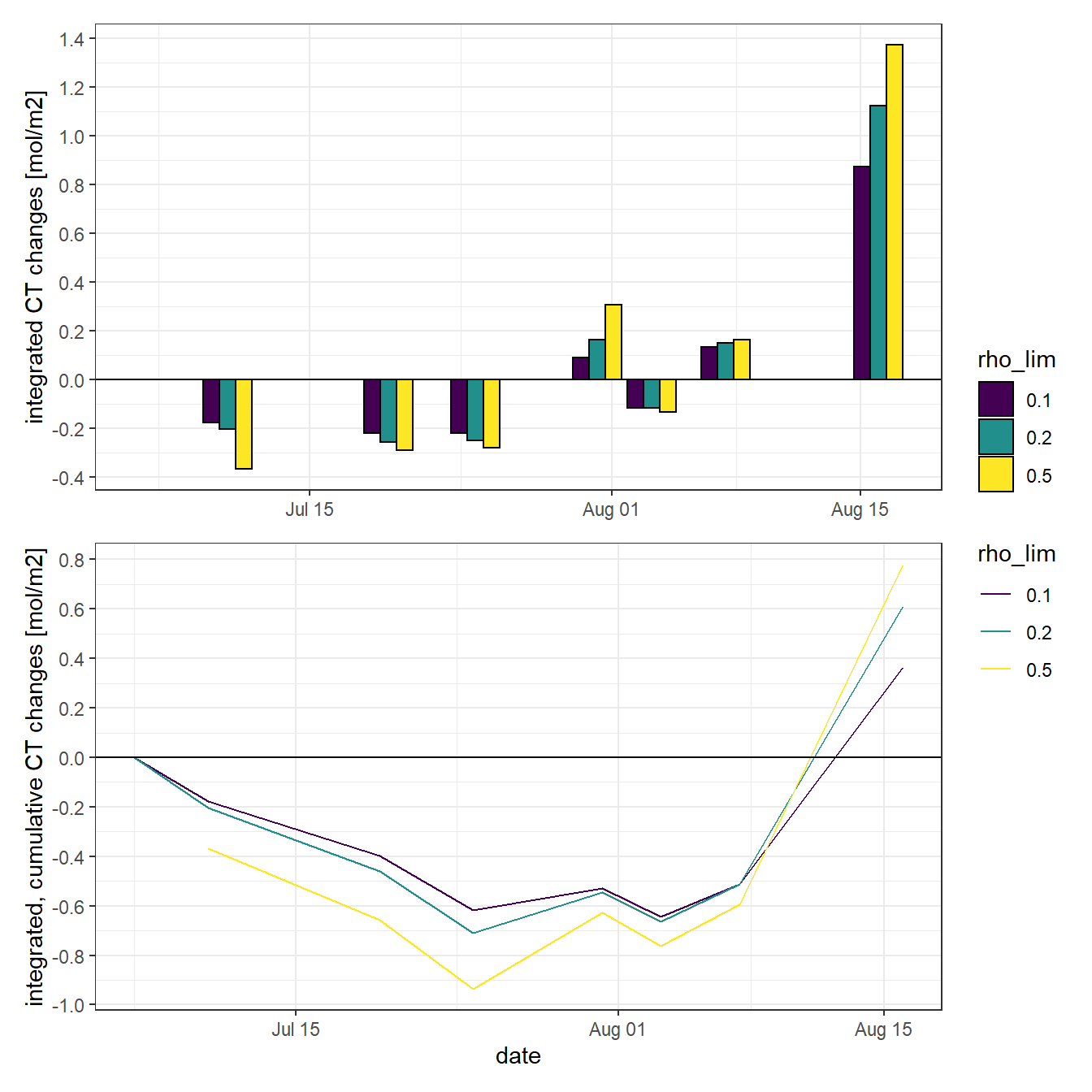
rm(p_iCT, p_iCT_cum)

ts_profiles_ID_surface_MLD <- ts_profiles_ID_surface
rm(ts_profiles_ID, ts_profiles_ID_surface)
4 CT profile reconstruction
4.1 Read data
ts_profiles_ID <-
  read_csv(here::here("Data/_merged_data_files", "ts_profiles_ID.csv"))

ts_profiles_ID <- ts_profiles_ID %>%
  mutate(CT = if_else(dep == 3.5, CT, NaN),
         ID = as.factor(ID)) %>%
  select(-date_ID)
4.2 CT vs temperature
As primary production (negative changes in CT) and increase in seawater temperature have a common driver (light), the relation between both changes was investigated.
ts_profiles_ID_diff <- ts_profiles_ID %>%
  drop_na() %>%
  arrange(date_time_ID) %>%
  mutate(CT_diff = CT - lag(CT, default = first(CT)),
         tem_diff = tem - lag(tem, default = first(tem)),
         factor = CT_diff / tem_diff,
         factor = if_else(is.na(factor), 0, factor))

ts_profiles_ID_diff %>%
  ggplot(aes(tem_diff, CT_diff))+
  geom_hline(yintercept = 0)+
  geom_vline(xintercept = 0)+
  geom_path()+
  geom_point()
4.3 Reconstruction of CT dynamics
The ratio of the incremental change of CT with temperature at the seasurface was applied to calculate the CT in other water depth based on the known change in temperature.
ts_profiles_ID_diff <- ts_profiles_ID_diff %>%
  select(ID, factor)

ts_profiles_ID <- full_join(ts_profiles_ID, ts_profiles_ID_diff)
rm(ts_profiles_ID_diff)

ts_profiles_ID <- ts_profiles_ID %>%
  arrange(date_time_ID) %>%
  group_by(dep) %>%
  mutate(tem_diff = tem - lag(tem, default = first(tem))) %>%
  ungroup()

ts_profiles_ID <- ts_profiles_ID %>%
  mutate(CT_diff = tem_diff * factor) %>%
  select(-factor)
The reconstructed incremental changes are added up to derive cummulative CT changes throughout the water column.
ts_profiles_ID_long <- ts_profiles_ID %>%
  select(ID, date_time_ID, dep, tem = tem_diff, CT = CT_diff) %>%
  pivot_longer(4:5, names_to = "var", values_to = "value_diff") %>%
  group_by(dep, var) %>%
  arrange(date_time_ID) %>%
  mutate(date_time_ID_diff = as.numeric(date_time_ID - lag(date_time_ID)),
         date_time_ID_ref  = date_time_ID - (date_time_ID - lag(date_time_ID))/2,
         value_diff_daily = value_diff / date_time_ID_diff,
         value_cum = cumsum(value_diff)) %>%
  ungroup()
4.4 Profiles of incremental changes
Changes of seawater parameters at each depth were reconstructed from one cruise day to the next and divided by the number of days inbetween.
ts_profiles_ID_long %>%
  arrange(dep) %>%
  ggplot(aes(value_diff, dep, col=ID))+
  geom_vline(xintercept = 0)+
  geom_point()+
  geom_path()+
  scale_y_reverse()+
  scale_color_viridis_d()+
  facet_wrap(~var, scales = "free_x")+
  labs(x="Change of value inbetween cruises per day")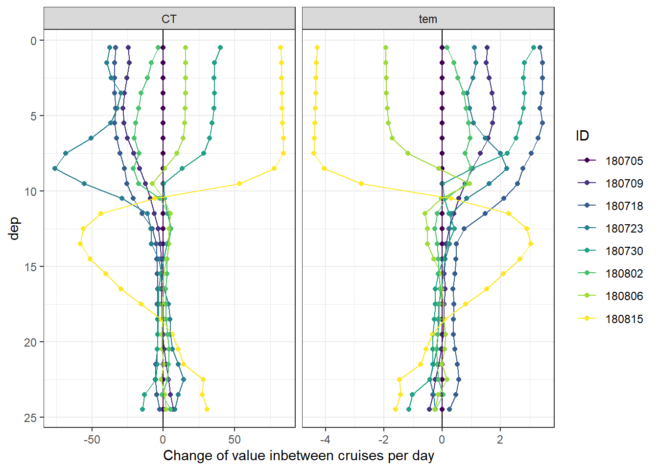
4.5 Profiles of cumulative changes
Cumulative changes of seawater parameters were calculated at each depth relative to the first cruise day on July 5.
ts_profiles_ID_long %>%
  arrange(dep) %>%
  ggplot(aes(value_cum, dep, col=ID))+
  geom_vline(xintercept = 0)+
  geom_point()+
  geom_path()+
  scale_y_reverse()+
  scale_color_viridis_d()+
  labs(x="Cumulative change of value")+
  facet_wrap(~var, scales = "free_x")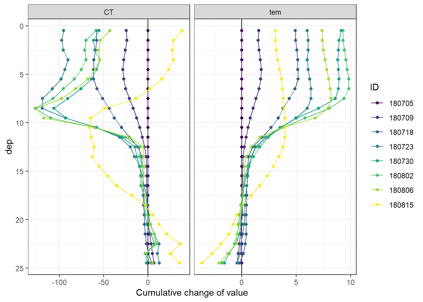
4.6 Hovmoeller plots
Hoevmoeller plots were generated for the reconstructed daily and cumulative changes in CT. Absolute values are not reproducible with this approach. Furthermore, it meets our expectations
4.6.1 Daily changes
bin_CT <- 2.5

ts_profiles_ID_long %>%
  filter(var == "CT") %>%
  ggplot()+
  geom_contour_fill(aes(x=date_time_ID_ref, y=dep, z=value_diff_daily),
                    breaks = MakeBreaks(bin_CT),
                    col="black")+
  geom_point(aes(x=date_time_ID, y=c(24.5)), size=3, shape=24, fill="white")+
  scale_fill_divergent(breaks = MakeBreaks(bin_CT),
                       guide = "colorstrip",
                       name="CT (µmol/kg)")+
  scale_y_reverse()+
  theme_bw()+
  labs(y="Depth (m)")+
  coord_cartesian(expand = 0)+
  theme(axis.title.x = element_blank(),
        axis.text.x = element_blank())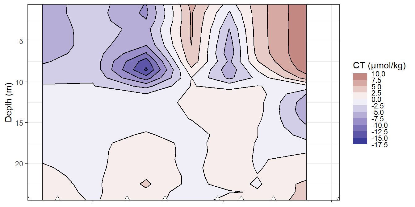
Hovmoeller plots of daily reconstructed changes in CT and temperature.
rm(bin_CT)4.6.2 Cumulative changes
bin_CT <- 20

ts_profiles_ID_long %>%
  filter(var == "CT") %>%
  ggplot()+
  geom_contour_fill(aes(x=date_time_ID, y=dep, z=value_cum),
                    breaks = MakeBreaks(bin_CT),
                    col="black")+
  geom_point(aes(x=date_time_ID, y=c(24.5)), size=3, shape=24, fill="white")+
  scale_fill_divergent(breaks = MakeBreaks(bin_CT),
                       guide = "colorstrip",
                       name="CT (µmol/kg)")+
  scale_y_reverse()+
  theme_bw()+
  labs(y="Depth (m)")+
  coord_cartesian(expand = 0)+
  theme(axis.title.x = element_blank(),
        axis.text.x = element_blank())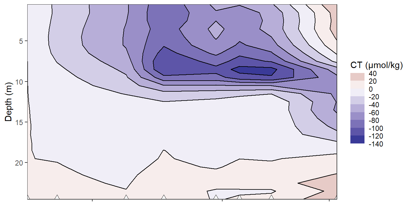
Hovmoeller plots of daily reconstructed changes in CT.
rm(bin_CT)4.7 iCT time series
Total incremental and cumulative CT changes inbetween cruise dates were calculated for the upper 10 m of the water body.
iCT_10 <- ts_profiles_ID_long %>%
  filter(dep < 17,
         var == "CT") %>%
  select(ID, date_time_ID, date_time_ID_ref, CT_diff=value_diff, CT_cum=value_cum) %>%
  group_by(ID, date_time_ID, date_time_ID_ref) %>%
  summarise(CT_i_diff = sum(CT_diff)/1000,
            CT_i_cum = sum(CT_cum)/1000) %>%
  ungroup()

iCT_10 %>%
  ggplot()+
  #geom_point(data = cruise_dates, aes(date_time_ID, 0), shape=21)+
  geom_col(aes(date_time_ID_ref, CT_i_diff),
           position = "dodge", alpha=0.3)+
  geom_line(aes(date_time_ID, CT_i_cum))+
  scale_color_viridis_d(name="Depth limit (m)")+
  scale_fill_viridis_d(name="Depth limit (m)")+
  labs(y="iCT [mol/m2]", x="")+
  theme_bw()
rm(ts_profiles_ID, ts_profiles_ID_long)5 Heat penetration depth
To investigate the link between temperature rise and CT drawdown, we estimated the mean penetration depth of both parameters, which was defined as the surface change (0-6m) devided by the integrated change across depth. To derive the integrated values, we summed up all negative changes in CT and temperature. For temperature we limited the integration to the depth at which the cummulative signal on July 23 was below 5% of the surface signal.
5.1 Read data
ts_profiles_ID_long_cum <-
  read_csv(here::here("Data/_merged_data_files", "ts_profiles_ID_long_cum.csv"))

ts_profiles_ID_long_cum <- ts_profiles_ID_long_cum %>%
  filter(var %in% c("CT", "tem")) %>%
  mutate(ID = as.factor(ID)) %>%
  select(-date_ID)
ts_profiles_ID <-
read_csv(here::here("Data/_merged_data_files", "ts_profiles_ID_long_cum_MLD.csv"))
ts_profiles_ID <- ts_profiles_ID %>%
filter(rho_lim == 0.1) %>%
select(ID, date_time_ID, dep, CT = value, CT_diff = value_diff, CT_cum = value_cum) %>%
mutate(ID = as.factor(ID))# surface values
diff_surface <- ts_profiles_ID_long_cum %>%
filter(dep < 6) %>%
group_by(ID, var) %>%
summarise(value_diff_surface = mean(value_diff, na.rm = TRUE),
value_cum_surface =mean(value_cum, na.rm = TRUE)) %>%
ungroup()
ts_profiles_ID_long_cum <- full_join(ts_profiles_ID_long_cum, diff_surface)
rm(diff_surface)
# directional changes in CT and tem
penetration_depth_CT <- ts_profiles_ID_long_cum %>%
filter(var == "CT") %>%
mutate(value_diff = if_else(value_diff<=0, value_diff, NaN),
value_cum = if_else(value_cum <=0, value_cum, NaN))
penetration_depth_tem <- ts_profiles_ID_long_cum %>%
filter(var == "tem") %>%
mutate(value_diff = if_else(value_diff>=0, value_diff, NaN),
value_cum = if_else(value_cum >=0, value_cum, NaN))
penetration_depth <- full_join(penetration_depth_CT,
penetration_depth_tem)
# define integration depth
integration_depth_tem <- penetration_depth_tem %>%
filter(ID == "180723") %>%
mutate(value_cum_rel = 100*value_cum/value_cum_surface)
integration_depth_tem %>%
ggplot(aes(value_cum_rel, dep))+
geom_vline(xintercept = c(5))+
geom_point()+
geom_path()+
scale_y_reverse(name = "Depth (m)")+
scale_x_continuous(breaks = seq(0,100,10),
name = "Cumulative temperature change relative to surface (%)")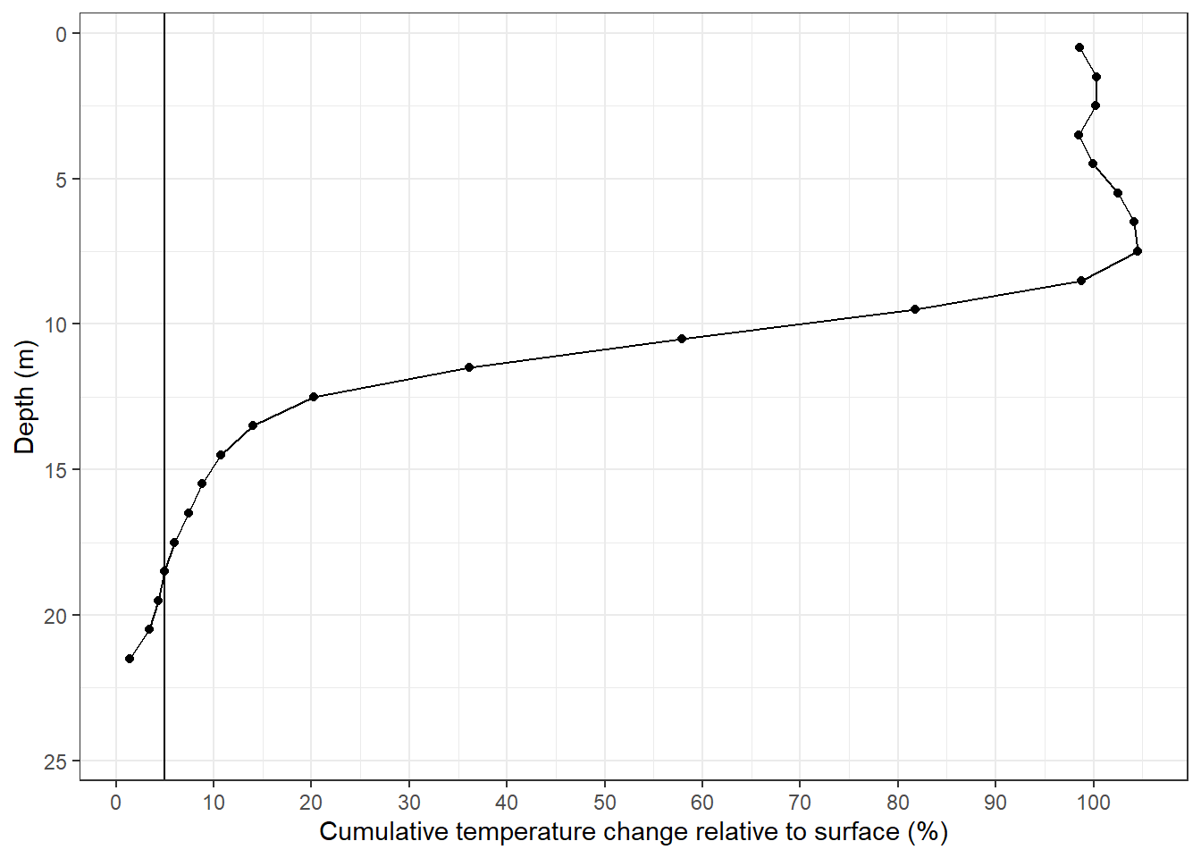
integration_depth_tem <- integration_depth_tem %>%
  filter(value_cum_rel < 5) %>%
  pull(dep) %>%
  min()

rm(penetration_depth_CT, penetration_depth_tem)
# calculate penetration depths
penetration_depth <- penetration_depth %>%
filter(dep < integration_depth_tem) %>%
group_by(var, ID, date_time_ID) %>%
summarise(value_diff_int = sum(value_diff, na.rm = TRUE),
value_cum_int = sum(value_cum, na.rm = TRUE),
value_diff_surface = mean(value_diff_surface, na.rm = TRUE),
value_cum_surface = mean(value_cum_surface, na.rm = TRUE),
penetration_depth_diff = value_diff_int/value_diff_surface,
penetration_depth_cum = value_cum_int/value_cum_surface) %>%
ungroup() %>%
filter(penetration_depth_diff > 0)
penetration_depth_mean <- penetration_depth %>%
group_by(var) %>%
summarise(penetration_depth_diff_mean = mean(penetration_depth_diff, na.rm=TRUE),
penetration_depth_cum_mean = mean(penetration_depth_cum, na.rm=TRUE),
penetration_depth_diff_sd = sd(penetration_depth_diff, na.rm=TRUE),
penetration_depth_cum_sd = sd(penetration_depth_cum, na.rm=TRUE)) %>%
ungroup()
penetration_depth_mean# A tibble: 2 x 5
var penetration_depth~ penetration_dept~ penetration_dept~ penetration_dept~
<chr> <dbl> <dbl> <dbl> <dbl>
1 CT 10.2 10.4 1.01 0.393
2 tem 11.3 10.6 2.43 0.608p_pene_diff <- penetration_depth %>%
ggplot(aes(date_time_ID, penetration_depth_diff, col=var))+
geom_hline(yintercept = 0)+
geom_hline(data = penetration_depth_mean,
aes(yintercept = penetration_depth_diff_mean,
col=var, linetype = "mean"))+
geom_line(aes(linetype="cruise"))+
geom_point()+
scale_y_reverse(name = "Penetration depth (m)", breaks = seq(0,20,5))+
scale_color_brewer(palette = "Set1", direction = -1)+
labs(title = "Incremental CT and temperature changes")+
theme(axis.title.x = element_blank(),
axis.text.x = element_blank(),
legend.title = element_blank())
p_pene_cum <- penetration_depth %>%
ggplot(aes(date_time_ID, penetration_depth_cum, col=var))+
geom_hline(yintercept = 0)+
geom_hline(data = penetration_depth_mean,
aes(yintercept = penetration_depth_cum_mean,
col=var, linetype = "mean"))+
geom_line(aes(linetype="cruise"))+
geom_point()+
scale_y_reverse(name = "Penetration depth (m)", breaks = seq(0,20,5))+
scale_color_brewer(palette = "Set1", direction = -1)+
labs(title = "Cumulative CT and temperature changes")+
theme(axis.title.x = element_blank(),
legend.title = element_blank())
p_pene_diff / p_pene_cum +
plot_layout(guides = "collect")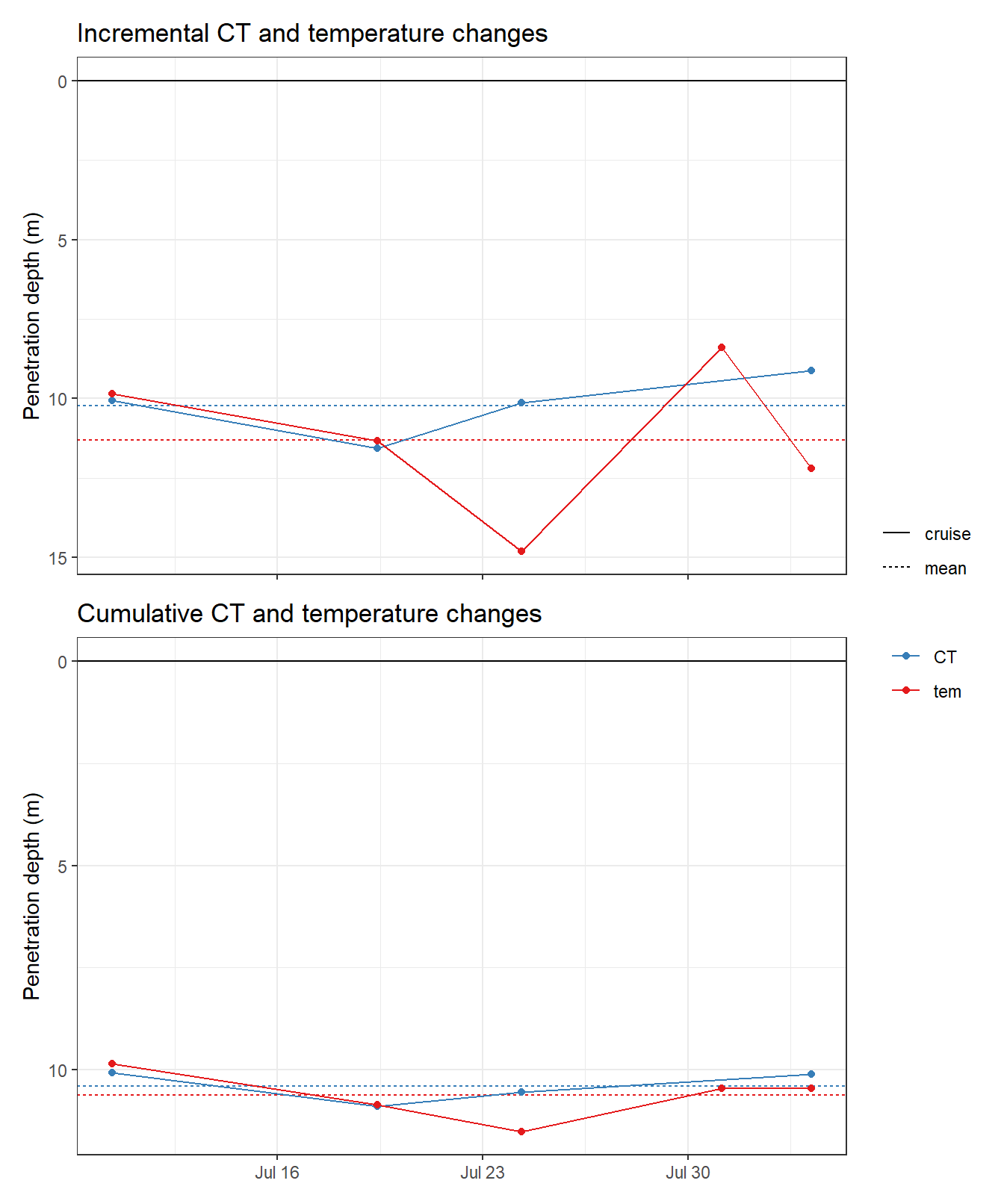
rm(p_pene_cum, p_pene_diff)5.2 iCT calculation
Integrated CT depletion was calculated as the product of observed incremental CT changes in surface waters and the respective mixed layer depth.
penetration_depth <- penetration_depth %>%
  filter(var == "tem") %>%
  select(ID, penetration_depth_diff)

ts_profiles_ID_zeff <- full_join(ts_profiles_ID, penetration_depth)

ts_profiles_ID_zeff_surface <- ts_profiles_ID_zeff %>%
  filter(dep==3.5) %>%
  arrange(date_time_ID) %>%
  mutate(iCT_diff = CT_diff * 11.3 / 1000,
         iCT_cum = cumsum(replace_na(iCT_diff, 0))) %>%
  ungroup()
p_iCT <- ts_profiles_ID_zeff_surface %>%
ggplot(aes(date_time_ID, iCT_diff))+
geom_hline(yintercept = 0)+
geom_col(col="black", position = "dodge")+
scale_y_continuous(breaks = seq(-100, 100, 0.2))+
#scale_fill_viridis_d()+
labs(y="integrated CT changes [mol/m2]")+
theme(axis.title.x = element_blank())
p_iCT_cum <- ts_profiles_ID_zeff_surface %>%
ggplot(aes(date_time_ID, iCT_cum))+
geom_line()+
geom_hline(yintercept = 0)+
scale_color_viridis_d()+
scale_y_continuous(breaks = seq(-100, 100, 0.2))+
theme(strip.background = element_blank(),
strip.text = element_blank())+
labs(y="integrated, cumulative CT changes [mol/m2]", x="date")
(p_iCT / p_iCT_cum)+
plot_layout(guides = 'collect')
rm(p_iCT, p_iCT_cum)

#rm(ts_profiles_ID, ts_profiles_ID_surface)
6 Comparison of approaches
iCT_10_flux_mix <-
  read_csv(here::here("Data/_merged_data_files", "ts_NCP_cum.csv"))

iCT_10_flux_mix <- iCT_10_flux_mix %>%
  filter(!is.na(CT_i_diff))
ggplot()+
geom_line(data = ts_profiles_ID_zeff_surface,
aes(date_time_ID, iCT_cum, col="zeff"))+
geom_line(data = ts_profiles_ID_surface_MLD %>% filter(rho_lim == 0.1),
aes(date_time_ID, iCT_cum, col="Rho 0.1"))+
geom_line(data = iCT_10,
aes(date_time_ID, CT_i_cum, col="CT recon"))+
geom_line(data = iCT_10_flux_mix,
aes(date_time, CT_i_cum, col="best guess"))+
geom_hline(yintercept = 0)+
scale_color_brewer(palette = "Set1", name="Estimate")+
scale_y_continuous(breaks = seq(-100, 100, 0.2))+
scale_x_datetime(breaks = "week",
date_labels = "%b %d")+
theme(axis.title.x = element_blank())+
labs(y="integrated, cumulative CT changes [mol/m2]")
sessionInfo()R version 3.6.3 (2020-02-29)
Platform: i386-w64-mingw32/i386 (32-bit)
Running under: Windows 10 x64 (build 18363)
Matrix products: default
locale:
[1] LC_COLLATE=English_Germany.1252 LC_CTYPE=English_Germany.1252
[3] LC_MONETARY=English_Germany.1252 LC_NUMERIC=C
[5] LC_TIME=English_Germany.1252
attached base packages:
[1] stats graphics grDevices utils datasets methods base
other attached packages:
[1] lubridate_1.7.4 metR_0.6.0 patchwork_1.0.0 marelac_2.1.10
[5] shape_1.4.4 seacarb_3.2.13 oce_1.2-0 gsw_1.0-5
[9] testthat_2.3.2 forcats_0.5.0 stringr_1.4.0 dplyr_0.8.5
[13] purrr_0.3.3 readr_1.3.1 tidyr_1.0.2 tibble_3.0.0
[17] ggplot2_3.3.0 tidyverse_1.3.0 workflowr_1.6.1
loaded via a namespace (and not attached):
[1] Rcpp_1.0.4 whisker_0.4 knitr_1.28 xml2_1.3.0
[5] magrittr_1.5 hms_0.5.3 rvest_0.3.5 tidyselect_1.0.0
[9] viridisLite_0.3.0 here_0.1 colorspace_1.4-1 lattice_0.20-41
[13] R6_2.4.1 rlang_0.4.5 fansi_0.4.1 broom_0.5.5
[17] xfun_0.12 dbplyr_1.4.2 modelr_0.1.6 withr_2.1.2
[21] git2r_0.26.1 ellipsis_0.3.0 htmltools_0.4.0 assertthat_0.2.1
[25] rprojroot_1.3-2 digest_0.6.25 lifecycle_0.2.0 haven_2.2.0
[29] rmarkdown_2.1 sp_1.4-1 compiler_3.6.3 cellranger_1.1.0
[33] pillar_1.4.3 scales_1.1.0 backports_1.1.5 generics_0.0.2
[37] jsonlite_1.6.1 httpuv_1.5.2 pkgconfig_2.0.3 rstudioapi_0.11
[41] munsell_0.5.0 highr_0.8 plyr_1.8.6 httr_1.4.1
[45] tools_3.6.3 grid_3.6.3 nlme_3.1-145 data.table_1.12.8
[49] gtable_0.3.0 checkmate_2.0.0 utf8_1.1.4 DBI_1.1.0
[53] cli_2.0.2 readxl_1.3.1 yaml_2.2.1 crayon_1.3.4
[57] RColorBrewer_1.1-2 farver_2.0.3 later_1.0.0 promises_1.1.0
[61] fs_1.4.0 vctrs_0.2.4 memoise_1.1.0 glue_1.3.2
[65] evaluate_0.14 labeling_0.3 reprex_0.3.0 stringi_1.4.6