Merging and interpolation of observations
Jens Daniel Müller
19 December, 2019
Last updated: 2019-12-19
Checks: 7 0
Knit directory: BloomSail/
This reproducible R Markdown analysis was created with workflowr (version 1.5.0). The Checks tab describes the reproducibility checks that were applied when the results were created. The Past versions tab lists the development history.
Great! Since the R Markdown file has been committed to the Git repository, you know the exact version of the code that produced these results.
Great job! The global environment was empty. Objects defined in the global environment can affect the analysis in your R Markdown file in unknown ways. For reproduciblity it’s best to always run the code in an empty environment.
The command set.seed(20191021) was run prior to running the code in the R Markdown file. Setting a seed ensures that any results that rely on randomness, e.g. subsampling or permutations, are reproducible.
Great job! Recording the operating system, R version, and package versions is critical for reproducibility.
Nice! There were no cached chunks for this analysis, so you can be confident that you successfully produced the results during this run.
Great job! Using relative paths to the files within your workflowr project makes it easier to run your code on other machines.
Great! You are using Git for version control. Tracking code development and connecting the code version to the results is critical for reproducibility. The version displayed above was the version of the Git repository at the time these results were generated.
Note that you need to be careful to ensure that all relevant files for the analysis have been committed to Git prior to generating the results (you can use wflow_publish or wflow_git_commit). workflowr only checks the R Markdown file, but you know if there are other scripts or data files that it depends on. Below is the status of the Git repository when the results were generated:
Ignored files:
    Ignored:    .Rhistory
    Ignored:    .Rproj.user/
    Ignored:    data/Maps/
    Ignored:    data/TinaV/
    Ignored:    data/_merged_data_files/
    Ignored:    data/_summarized_data_files/
Note that any generated files, e.g. HTML, png, CSS, etc., are not included in this status report because it is ok for generated content to have uncommitted changes.
There are no past versions. Publish this analysis with wflow_publish() to start tracking its development.
library(tidyverse)
library(lubridate)
library(zoo)
# library(dygraphs)
# library(xts)
CTD and pCO2 data
Merging summarized data sets
# Load Sensor and HydroC data ---------------------------------------------

CTD <- read_csv(here::here("Data/_summarized_data_files",
                              "Tina_V_Sensor_Profiles_Transects.csv"),
                   col_types = list("pCO2" = col_double())) %>%
  rename(pCO2_analog = pCO2)

HC <- read_csv(here::here("Data/_summarized_data_files", "Tina_V_HydroC.csv"))
HC_full <- read_csv(here::here("Data/_summarized_data_files", "Tina_V_HydroC_full.csv"))

# Time offset correction ----------------------------------------------

# Time offset was determined by comparing zeroing reads from Sensor and HC
# in the plots produced in the section Time stamp synchronzity below
# before applying this correction

CTD <- CTD %>%
  mutate(day = yday(date_time),
         date_time = if_else(day >= 206 & day <= 220,
                             date_time - 80, date_time - 10)) %>%
  select(-day)

# Merge Sensor and HydroC data --------------------------------------------

df <- full_join(CTD, HC) %>%
  arrange(date_time)

df_full <- full_join(CTD, HC_full) %>%
  arrange(date_time)

rm(HC, HC_full, CTD)
Interpolation to common time stamp
CTD and auxillary recordings (15 sec measurment interval) are interpolated to HydroC time stamps (first 10 sec, than 1 sec measurement interval) when gaps between observations are not larger than 20. Thereafter, HydroC readings not falling in regular transects/profilings are removed, by removing rows with NA depth values. Furthermore, CTD readings without corresponding HydroC reading are removed, except during periods when HydroC was not operating.
# Interpolate Sensor data to HydroC timestamp

df <-
  df %>%
  mutate(dep = na.approx(dep, na.rm = FALSE, maxgap = 20),
         sal = na.approx(sal, na.rm = FALSE, maxgap = 20),
         tem = na.approx(tem, na.rm = FALSE, maxgap = 20),
         pCO2_analog = na.approx(pCO2_analog, na.rm = FALSE, maxgap = 20),
         pH = na.approx(pH, na.rm = FALSE, maxgap = 20),
         V_pH = na.approx(V_pH, na.rm = FALSE, maxgap = 20),
         O2 = na.approx(O2, na.rm = FALSE, maxgap = 20),
         Chl = na.approx(Chl, na.rm = FALSE, maxgap = 20)) %>%
  filter(!is.na(dep)) %>% #remove HC readings not falling in regular transects/profilings
  fill(ID, type, station) %>%
  filter(!is.na(deployment) | is.na(pCO2_analog)) # removes CTD readings without corresponding HydroC reading, except during periods when HydroC was not operating

df_full <-
  df_full %>%
  mutate(dep = na.approx(dep, na.rm = FALSE, maxgap = 20),
         sal = na.approx(sal, na.rm = FALSE, maxgap = 20),
         tem = na.approx(tem, na.rm = FALSE, maxgap = 20),
         pCO2_analog = na.approx(pCO2_analog, na.rm = FALSE, maxgap = 20),
         pH = na.approx(pH, na.rm = FALSE, maxgap = 20),
         V_pH = na.approx(V_pH, na.rm = FALSE, maxgap = 20),
         O2 = na.approx(O2, na.rm = FALSE, maxgap = 20),
         Chl = na.approx(Chl, na.rm = FALSE, maxgap = 20)) %>%
  filter(!is.na(dep)) %>% #remove HC readings not falling in regular transects/profilings
  fill(ID, type, station) %>%
  filter(!is.na(deployment) | is.na(pCO2_analog)) # removes CTD readings without corresponding HydroC reading, except during periods when HydroC was not operating

# Time stamp synchronzity -------------------------------------------------
#
# df <- df %>%
#   mutate(day = yday(date_time))
#
# for (dayID in unique(df$day)) {
#
#   df %>%
#     filter(day == dayID) %>%
#       ggplot()+
#       geom_point(aes(date_time, pCO2, col="HC"))+
#       geom_point(aes(date_time, dep, col="dep"))+
#       geom_point(aes(date_time, pH, col="pH"))+
#       geom_point(aes(date_time, pCO2_analog, col="Sensor_int"))
#
#     ggsave(here::here("/Plots/TinaV/Sensor/HydroC_diagnostics/Timing/day",
#                       paste(dayID,"_day_HydroC_merged.jpg", sep="")),
#            width = 10, height = 4)
# }
#
#
# for (depID in unique(df$deployment)) {
#
#   df_dep <- df %>%
#     filter(deployment == depID, Zero == 1)
#
#   for (zerID in unique(df_dep$Zero_ID)) {
#
#     df_dep %>%
#       filter(Zero_ID == zerID) %>%
#       ggplot()+
#       geom_point(aes(date_time, pCO2, col="HC"))+
#       geom_point(aes(date_time, pCO2_analog, col="Sensor_int"))
#
#     ggsave(here::here("/Plots/TinaV/Sensor/HydroC_diagnostics/Timing/Zeroing",
#                       paste(depID,"_deployment_",zerID,"_Zero_ID_HydroC.jpg", sep="")),
#            width = 10, height = 4)
#
#   }
# }
write_csv(df, here::here("Data/_merged_data_files", "BloomSail_CTD_HydroC.csv"))
write_csv(df_full, here::here("Data/_merged_data_files", "BloomSail_CTD_HydroC_full.csv"))
rm(df, df_full)df <- read_csv(here::here("data/_merged_data_files",
"BloomSail_CTD_HydroC.csv"),
col_types = cols(ID = col_character(),
pCO2_analog = col_double(),
pCO2 = col_double(),
Zero = col_factor(),
Flush = col_factor(),
Zero_ID = col_integer(),
deployment = col_integer(),
duration = col_double(),
mixing = col_character()))
df %>%
filter(!is.na(pCO2)) %>%
ggplot()+
geom_path(aes(date_time, pCO2, col = "HydroC, drift corrected"))+
geom_path(aes(date_time, pCO2_analog, col = "analog CTD"))+
scale_color_brewer(palette = "Set1", name = "pCO2 record")+
labs(y=expression(pCO[2]~(µatm)), x="")+
facet_wrap(~ID, scales = "free_x", ncol = 1)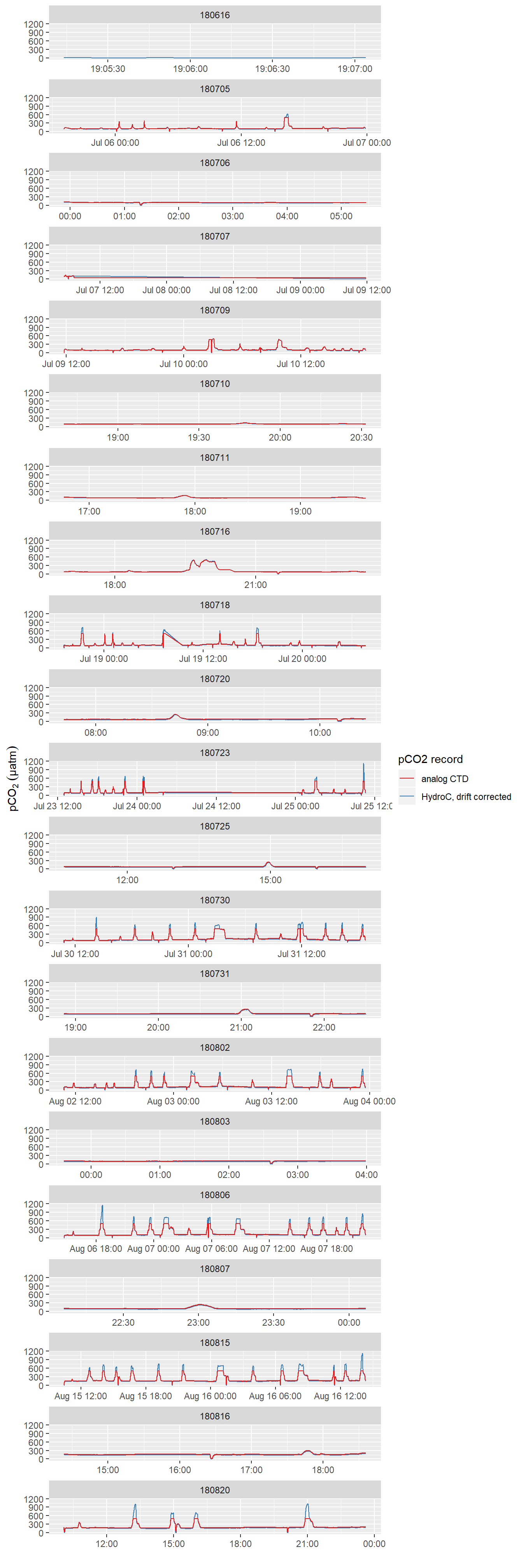
pCO2 record after interpolation to HydroC timestamp (analog output from HydroC and drift corrected data provided by Contos). ID refers to the starting date of each cruise. Please note that pCO2 measurement range is restricted to 100-500 µatm here due to the settings of the analog voltage output of the sensor. Zeroing periods are included.
# ts <- xts(cbind(df$pCO2, df$dep), order.by = df$date_time)
# names(ts) <- c("pCO2", "Depth")
#
# ts %>%
#   dygraph() %>%
#   dyRangeSelector() %>% #dateWindow = c("2012-01-01", "2016-12-31")
#   dySeries("pCO2", label = "pCO2") %>%
#   dySeries("Depth", axis = 'y2', label = "Depth") %>%
#   dyAxis("y", label = "pCO2 [µatm]") %>%
#   dyAxis("y2", label = "Depth [m]") %>%
#   dyOptions(drawPoints = TRUE, pointSize = 1)
Sensor and track data
Sensor <- read_csv(here::here("data/_merged_data_files",
                          "BloomSail_CTD_HydroC.csv"),
               col_types = cols(ID = col_character(),
                                pCO2_analog = col_double(),
                                pCO2 = col_double(),
                                Zero = col_factor(),
                                Flush = col_factor(),
                                Zero_ID = col_integer(),
                                deployment = col_integer(),
                                duration = col_double(),
                                mixing = col_character()))


track <-
  read_csv(here::here("Data/_summarized_data_files",
                       "TinaV_Track.csv"))


df <- full_join(Sensor, track) %>%
  arrange(date_time)

# interpolate track data and than remove columns that originate from track time stamp
df <-
  df %>%
  mutate(lat = na.approx(lat, na.rm = FALSE, maxgap = 20),
         lon = na.approx(lon, na.rm = FALSE, maxgap = 20)) %>%
  filter(!is.na(dep))

df %>%
  write_csv(here::here("Data/_merged_data_files", "BloomSail_CTD_HydroC_track.csv"))

rm(df)
```
Tasks / open questions
- Check interpolation to CTD Sensor timestamp as alternative option
sessionInfo()R version 3.5.0 (2018-04-23)
Platform: x86_64-w64-mingw32/x64 (64-bit)
Running under: Windows 10 x64 (build 18363)
Matrix products: default
locale:
[1] LC_COLLATE=English_United States.1252
[2] LC_CTYPE=English_United States.1252
[3] LC_MONETARY=English_United States.1252
[4] LC_NUMERIC=C
[5] LC_TIME=English_United States.1252
attached base packages:
[1] stats graphics grDevices utils datasets methods base
other attached packages:
[1] zoo_1.8-6 lubridate_1.7.4 forcats_0.4.0 stringr_1.4.0
[5] dplyr_0.8.3 purrr_0.3.3 readr_1.3.1 tidyr_1.0.0
[9] tibble_2.1.3 ggplot2_3.2.1 tidyverse_1.3.0
loaded via a namespace (and not attached):
[1] tidyselect_0.2.5 xfun_0.10 haven_2.2.0
[4] lattice_0.20-35 colorspace_1.4-1 vctrs_0.2.0
[7] generics_0.0.2 htmltools_0.4.0 yaml_2.2.0
[10] rlang_0.4.1 later_1.0.0 pillar_1.4.2
[13] withr_2.1.2 glue_1.3.1 DBI_1.0.0
[16] RColorBrewer_1.1-2 dbplyr_1.4.2 modelr_0.1.5
[19] readxl_1.3.1 lifecycle_0.1.0 munsell_0.5.0
[22] gtable_0.3.0 workflowr_1.5.0 cellranger_1.1.0
[25] rvest_0.3.5 evaluate_0.14 labeling_0.3
[28] knitr_1.25 httpuv_1.5.2 highr_0.8
[31] broom_0.5.2 Rcpp_1.0.2 promises_1.1.0
[34] backports_1.1.5 scales_1.0.0 jsonlite_1.6
[37] fs_1.3.1 hms_0.5.2 digest_0.6.22
[40] stringi_1.4.3 grid_3.5.0 rprojroot_1.3-2
[43] here_0.1 cli_1.1.0 tools_3.5.0
[46] magrittr_1.5 lazyeval_0.2.2 crayon_1.3.4
[49] pkgconfig_2.0.3 zeallot_0.1.0 xml2_1.2.2
[52] reprex_0.3.0 rstudioapi_0.10 assertthat_0.2.1
[55] rmarkdown_1.17 httr_1.4.1 R6_2.4.0
[58] nlme_3.1-137 git2r_0.26.1 compiler_3.5.0