GLODAP subset variable climate A
Jens Daniel Müller
02 March, 2021
Last updated: 2021-03-02
Checks: 7 0
Knit directory: RECCAP2_CESM_ETHZ_submission/
This reproducible R Markdown analysis was created with workflowr (version 1.6.2). The Checks tab describes the reproducibility checks that were applied when the results were created. The Past versions tab lists the development history.
Great! Since the R Markdown file has been committed to the Git repository, you know the exact version of the code that produced these results.
Great job! The global environment was empty. Objects defined in the global environment can affect the analysis in your R Markdown file in unknown ways. For reproduciblity it’s best to always run the code in an empty environment.
The command set.seed(20210113) was run prior to running the code in the R Markdown file. Setting a seed ensures that any results that rely on randomness, e.g. subsampling or permutations, are reproducible.
Great job! Recording the operating system, R version, and package versions is critical for reproducibility.
Nice! There were no cached chunks for this analysis, so you can be confident that you successfully produced the results during this run.
Great job! Using relative paths to the files within your workflowr project makes it easier to run your code on other machines.
Great! You are using Git for version control. Tracking code development and connecting the code version to the results is critical for reproducibility.
The results in this page were generated with repository version 5611ec5. See the Past versions tab to see a history of the changes made to the R Markdown and HTML files.
Note that you need to be careful to ensure that all relevant files for the analysis have been committed to Git prior to generating the results (you can use wflow_publish or wflow_git_commit). workflowr only checks the R Markdown file, but you know if there are other scripts or data files that it depends on. Below is the status of the Git repository when the results were generated:
Ignored files:
    Ignored:    .Rhistory
    Ignored:    .Rproj.user/

Untracked files:
    Untracked:  analysis/diagnostics.Rmd
    Untracked:  code/Workflowr_project_managment.R
    Untracked:  data/overview/
    Untracked:  data/regions/
Note that any generated files, e.g. HTML, png, CSS, etc., are not included in this status report because it is ok for generated content to have uncommitted changes.
These are the previous versions of the repository in which changes were made to the R Markdown (analysis/time_series.Rmd) and HTML (docs/time_series.html) files. If you’ve configured a remote Git repository (see ?wflow_git_remote), click on the hyperlinks in the table below to view the files as they were in that past version.
| File | Version | Author | Date | Message |
|---|---|---|---|---|
| Rmd | 5611ec5 | jens-daniel-mueller | 2021-03-02 | maps and time series of 2D data |
| html | 6e5c0fd | jens-daniel-mueller | 2021-03-02 | Build site. |
| Rmd | edfb67c | jens-daniel-mueller | 2021-03-02 | plot spatially integrated time series |
| html | 026469a | jens-daniel-mueller | 2021-03-02 | Build site. |
| Rmd | 7ee6e95 | jens-daniel-mueller | 2021-03-02 | plot spatially integrated time series |
path_cmorized_annual <-
  "/nfs/kryo/work/loher/CESM_output/RECCAP2/submit_Dec2020/split/"
1 Region masks
region_masks_all <-
  read_csv("data/regions/RECCAP2_region_masks_all_clean.cvs")
2 File names
overview <-
  read_csv("data/overview/overview_files.csv")
3 Time series plots
3.1 iT
Comments:
- fgco2_reg
- regions not accessible
- values seem identical to fgco2_glob
# set name of model to be subsetted
experiment_IDs <- c("A", "B", "C", "D")

# for loop across variables
variables <-
  c(
    "fgco2_glob"
    # "fgco2_reg"
  )

for (i_experiment_ID in experiment_IDs) {
  for (i_variable in variables) {

    # i_experiment_ID <- experiment_IDs[1]
    # i_variable <- variables[1]

    # read list of all files
    file <- paste(i_variable,
                  "_CESM-ETHZ_",
                  i_experiment_ID,
                  "_1_gr_1980-2018.nc",
                  sep = "")
    print(file)

    # read in data
    variable_data <-
      tidync(paste(path_cmorized_annual,
                   file,
                   sep = ""))

    # convert to tibble
    variable_data_tibble <- variable_data %>%
      hyper_tibble()

    # remove open link to nc file
    rm(variable_data)

    print(
    variable_data_tibble %>%
      ggplot(aes(time_mon,
                 !!sym(i_variable))) +
      geom_path() +
      labs(title = paste("experiment_ID:", i_experiment_ID))
    )

  }
}
[1] "fgco2_glob_CESM-ETHZ_A_1_gr_1980-2018.nc"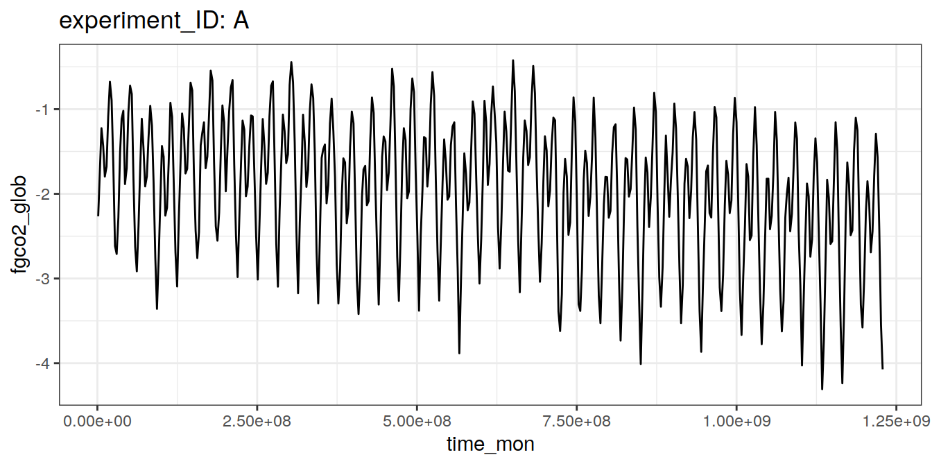
| Version | Author | Date |
|---|---|---|
| 6e5c0fd | jens-daniel-mueller | 2021-03-02 |
[1] "fgco2_glob_CESM-ETHZ_B_1_gr_1980-2018.nc"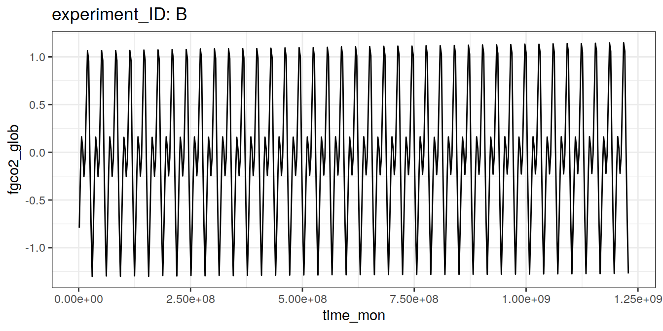
| Version | Author | Date |
|---|---|---|
| 6e5c0fd | jens-daniel-mueller | 2021-03-02 |
[1] "fgco2_glob_CESM-ETHZ_C_1_gr_1980-2018.nc"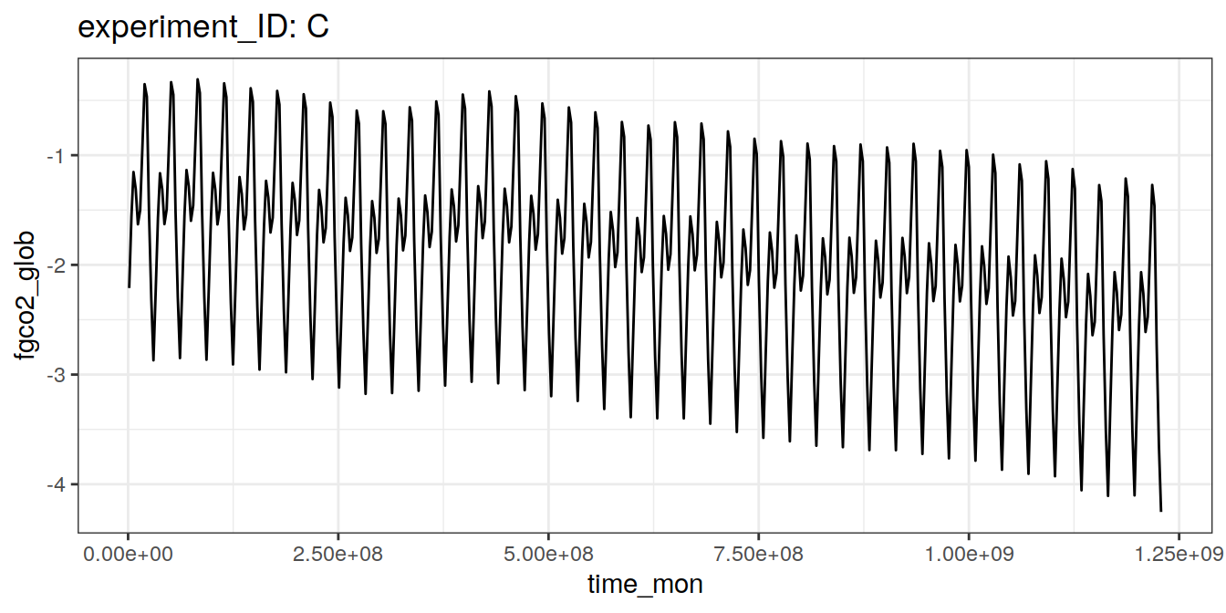
| Version | Author | Date |
|---|---|---|
| 6e5c0fd | jens-daniel-mueller | 2021-03-02 |
[1] "fgco2_glob_CESM-ETHZ_D_1_gr_1980-2018.nc"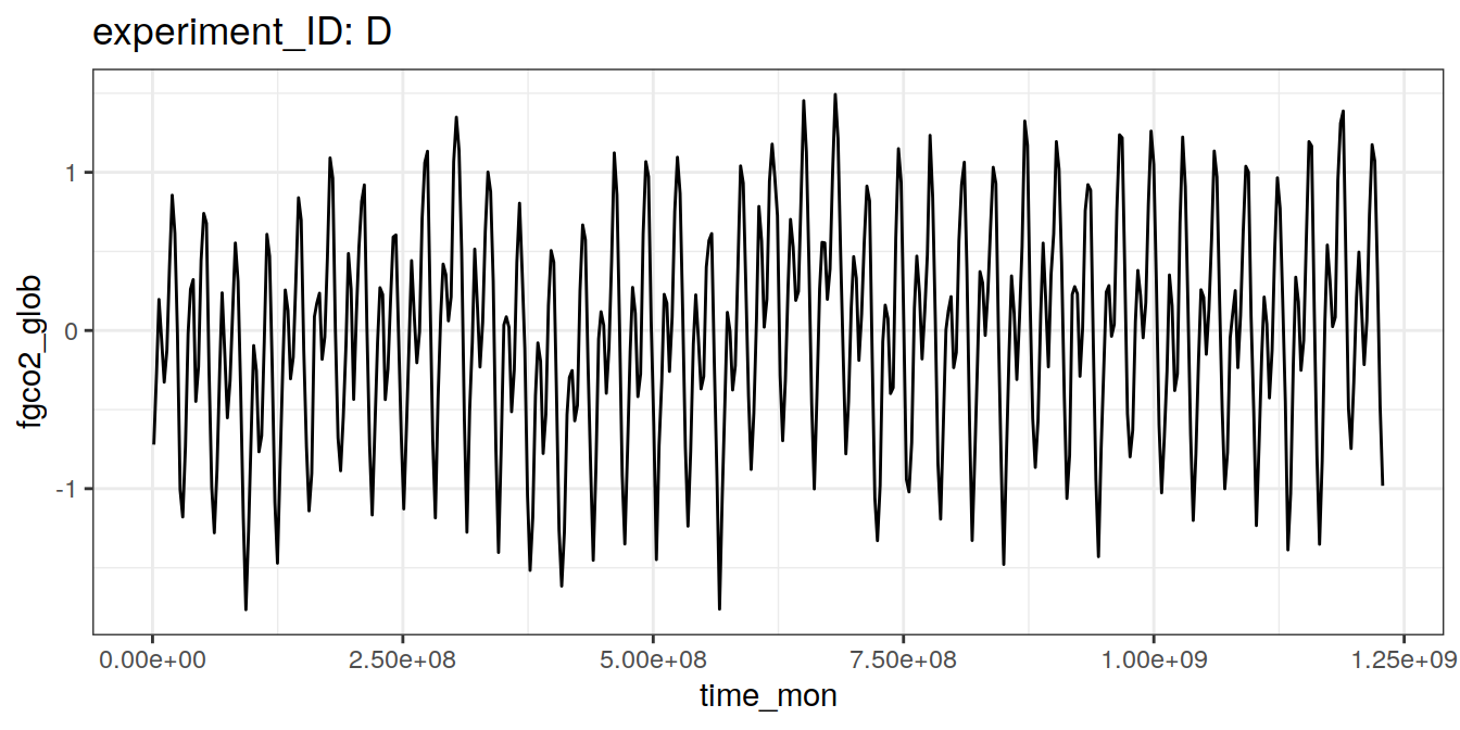
| Version | Author | Date |
|---|---|---|
| 6e5c0fd | jens-daniel-mueller | 2021-03-02 |
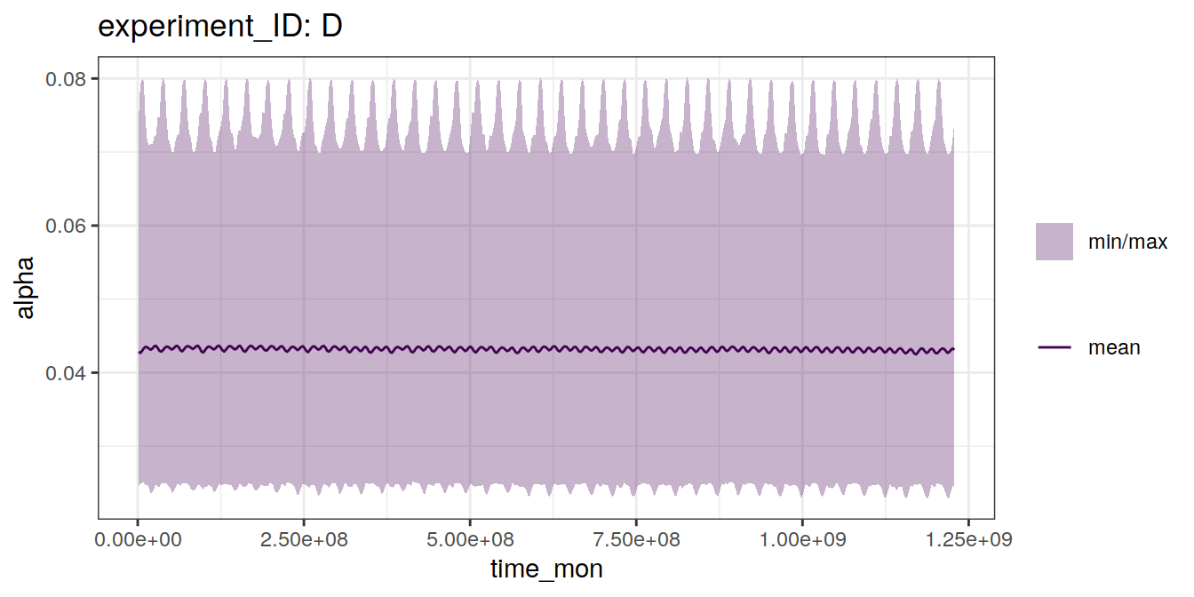
3.2 2D variables (XYT)
Comments:
# for loop across variables
variables <-
overview %>%
filter(shape == "XYT") %>%
distinct(variable_id) %>%
pull()
variables <- variables[1]
for (i_experiment_ID in experiment_IDs) {
for (i_variable in variables) {
# i_experiment_ID <- experiment_IDs[1]
# i_variable <- variables[1]
# read list of all files
file <- paste(i_variable,
"_CESM-ETHZ_",
i_experiment_ID,
"_1_gr_1980-2018.nc",
sep = "")
print(file)
# read in data
variable_data <-
tidync(paste(path_cmorized_annual,
file,
sep = ""))
# convert to tibble
variable_data_tibble <- variable_data %>%
hyper_tibble()
# remove open link to nc file
rm(variable_data)
variable_data_tibble_climatology <-
variable_data_tibble %>%
group_by(lat, lon) %>%
summarise(!!paste(sym(i_variable),"mean",sep = "_") := mean(!!sym(i_variable), na.rm = TRUE),
!!paste(sym(i_variable),"min",sep = "_") := min(!!sym(i_variable), na.rm = TRUE),
!!paste(sym(i_variable),"max",sep = "_") := max(!!sym(i_variable), na.rm = TRUE)) %>%
ungroup()
variable_data_tibble_climatology <- variable_data_tibble_climatology %>%
pivot_longer(starts_with(i_variable),
values_to = "value",
names_to = "parameter")
print(
variable_data_tibble_climatology %>%
ggplot(aes(lon, lat, fill=value)) +
geom_raster() +
scale_fill_viridis_c() +
coord_quickmap(expand = 0) +
facet_grid(.~parameter) +
theme(axis.title = element_blank()) +
labs(title = paste("experiment_ID:", i_experiment_ID))
)
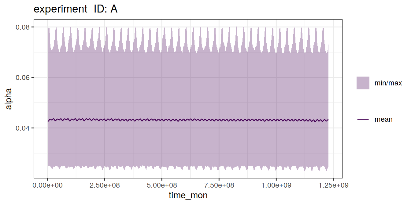
variable_data_tibble_time_series <-
variable_data_tibble %>%
group_by(time_mon) %>%
summarise("mean" := mean(!!sym(i_variable), na.rm = TRUE),
"min" := min(!!sym(i_variable), na.rm = TRUE),
"max" := max(!!sym(i_variable), na.rm = TRUE)) %>%
ungroup()
print(
variable_data_tibble_time_series %>%
ggplot() +
geom_ribbon(aes(
x = time_mon,
ymin = min,
ymax = max,
fill = "min/max"
), alpha = 0.3) +
geom_path(aes(
x = time_mon,
y = mean,
col = "mean"
)) +
scale_fill_viridis_d() +
scale_color_viridis_d() +
labs(title = paste("experiment_ID:", i_experiment_ID),
y = i_variable
) +
theme(legend.title = element_blank())
)
}
}[1] "alpha_CESM-ETHZ_A_1_gr_1980-2018.nc"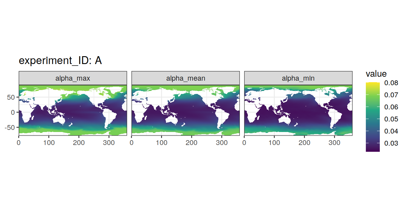
[1] "alpha_CESM-ETHZ_B_1_gr_1980-2018.nc"
[1] "alpha_CESM-ETHZ_C_1_gr_1980-2018.nc"

[1] "alpha_CESM-ETHZ_D_1_gr_1980-2018.nc"
# set name of model to be subsetted
experiment_ID <- "A"

# for loop across variables
variables <-
  c("fgco2",
    "spco2",
    "fice",
    "intpp",
    "epc100",
    "epc1000",
    "epc100type / epc1000type",
    "epcalc100",
    "Kw",
    "pco2atm",
    "alpha",
    "tos",
    "sos",
    "dissicos",
    "talkos",
    "no3os",
    "po4os",
    "sios",
    "dfeos",
    "o2os",
    "intphyc",
    "intphynd",
    "intdiac",
    "intzooc",
    "chlos",
    "mld",
    "zeu",
    "dissic",
    "talk",
    "thetao",
    "so",
    "epc",
    "no3",
    "po4",
    "si",
    "o2")

for (i_variable in variables) {
  # i_variable <- variables[1]

  # read list of all files
  file <- paste(i_variable,
                "_CESM-ETHZ_",
                experiment_ID,
                "_1_gr_1980-2018.nc",
                sep = "")
  print(file)

  # read in data
  variable_data <-
    read_ncdf(paste(path_cmorized_annual,
                    file,
                    sep = ""))

  # convert to tibble
  variable_data_tibble <- variable_data %>%
    select(-time_mon) %>%
    as_tibble()

  # remove open link to nc file
  rm(variable_data)

  # remove na values
  variable_data_tibble <-
    variable_data_tibble %>%
    filter(!is.na(!!sym(i_variable)))

  variable_data_tibble %>%
    ggplot(aes(time_mon, as.numeric(fgco2_glob))) +
    geom_path()

  # # harmonize longitudes
  # variable_data_tibble <- variable_data_tibble %>%
  #   mutate(lon = if_else(lon < 20, lon + 360, lon))

  # only consider model grids within basinmask
  variable_data_tibble <-
    inner_join(variable_data_tibble, basinmask) %>%
    select(-basin_AIP)

  # mutate variables
  variable_data_tibble <- variable_data_tibble %>%
    mutate(month = month(time_mon), !!sym(i_variable) := as.numeric(!!sym(i_variable))) %>%
    select(-time_mon)

  # calculate model summary stats
  stats <- variable_data_tibble %>%
    pull(!!sym(i_variable)) %>%
    summary()

  stats <- c(year = i_year, variable = i_variable, stats)

  if (exists("stats_summary")) {
    stats_summary <- bind_rows(stats_summary, stats)
  }

  if (!exists("stats_summary")) {
    stats_summary <- stats
  }

  rm(stats)

  # subset model at month x lat x lon grid of observations
  model_grid_horizontal <-
    inner_join(Glodap_year_grid_horizontal, variable_data_tibble)

  # join model and month x lat x lon x depth grid of observations
  model_obs <-
    full_join(model_grid_horizontal, Glodap_year_grid_depth)

  # calculate nr of observations per month x lat x lon grid
  model_obs <- model_obs %>%
    group_by(month, lat, lon) %>%
    mutate(n = sum(!is.na(!!sym(i_variable)))) %>%
    ungroup()

  # set variable value from model for observation depth, if only one model depth available
  model_obs_set <- model_obs %>%
    filter(n == 1) %>%
    group_by(lon, lat, month) %>%
    mutate(!!sym(i_variable) := mean(!!sym(i_variable), na.rm = TRUE)) %>%
    ungroup()

  # interpolate variable value from model to observation depth
  model_obs_interpo <- model_obs %>%
    filter(n > 1) %>%
    group_by(lon, lat, month) %>%
    arrange(depth) %>%
    mutate(!!sym(i_variable) := approxfun(depth, !!sym(i_variable), rule = 2)(depth)) %>%
    ungroup()

  # join interpolated and set model values
  model_obs_interpo <- full_join(model_obs_interpo, model_obs_set)
  rm(model_obs_set)

  # subsetted interpolated values at observation depth
  model_obs_interpo <-
    inner_join(Glodap_year_grid_depth, model_obs_interpo) %>%
    select(-n) %>%
    mutate(year = as.numeric(i_year))

  # select observation grids without corresponding model subset
  na_model <-
    full_join(Glodap_year_grid_depth, model_obs_interpo) %>%
    filter(is.na(!!sym(i_variable))) %>%
    select(month, lat, lon) %>%
    unique()

  # rename interpolated model variable to indicate as model output
  model_obs_interpo <- model_obs_interpo %>%
    rename(!!sym(paste(i_variable, "model", sep = "_")) := !!sym(i_variable))

  # add model subset to GLODAP
  GLODAP <-
    natural_join(
      GLODAP,
      model_obs_interpo,
      by = c("year", "month", "lat", "lon", "depth"),
      jointype = "FULL"
    )

  # calculate annual average variable
  variable_data_tibble_annual_average <- variable_data_tibble %>%
    fselect(-month) %>%
    fgroup_by(lat, lon, depth) %>% {
      add_vars(fgroup_vars(., "unique"),
               fmean(., keep.group_vars = FALSE))
    }

  # select surface annual average variable
  variable_data_tibble_annual_average_surface <-
    variable_data_tibble_annual_average %>%
    filter(depth == min(depth))

  # surface map of variable
  map +
    geom_raster(data = variable_data_tibble_annual_average_surface, aes(lon, lat, fill = !!sym(i_variable))) +
    scale_fill_viridis_c(name = i_variable) +
    geom_point(data = model_obs_interpo,
               aes(lon, lat), col = "black") +
    geom_point(data = na_model,
               aes(lon, lat), col = "red") +
    labs(
      title = "GLODAP-based cmorized subset distribution",
      subtitle = paste(
        "Model depth: 5m | Annual average of year",
        i_year,
        "| red = subsetting failed"
      ),
      x = "Longitude",
      y = "Latitude"
    )

  ggsave(
    paste(
      path_preprocessing,
      "regular_subset_distribution_runA/",
      i_variable,
      "_",
      i_year,
      ".png",
      sep = ""
    ),
    width = 5,
    height = 3
  )
}

}

# write raw data file for GLODAP-based subsetting model variables
GLODAP %>%
  write_csv(
    paste(
      path_preprocessing,
      "GLODAPv2.2020_preprocessed_model_runA_raw_subset.csv",
      sep = ""
    )
  )

# write file for model summary statistics (original cmorized unit)
stats_summary %>%
  write_csv(
    paste(
      path_preprocessing,
      "regular_subset_distribution_runA/",
      experiment_ID,
      "_summary_stats.csv",
      sep = ""
    )
  )
sessionInfo()R version 4.0.3 (2020-10-10)
Platform: x86_64-pc-linux-gnu (64-bit)
Running under: openSUSE Leap 15.2
Matrix products: default
BLAS: /usr/local/R-4.0.3/lib64/R/lib/libRblas.so
LAPACK: /usr/local/R-4.0.3/lib64/R/lib/libRlapack.so
locale:
[1] LC_CTYPE=en_US.UTF-8 LC_NUMERIC=C
[3] LC_TIME=en_US.UTF-8 LC_COLLATE=en_US.UTF-8
[5] LC_MONETARY=en_US.UTF-8 LC_MESSAGES=en_US.UTF-8
[7] LC_PAPER=en_US.UTF-8 LC_NAME=C
[9] LC_ADDRESS=C LC_TELEPHONE=C
[11] LC_MEASUREMENT=en_US.UTF-8 LC_IDENTIFICATION=C
attached base packages:
[1] stats graphics grDevices utils datasets methods base
other attached packages:
[1] tidync_0.2.4 stars_0.4-3 sf_0.9-6 abind_1.4-5
[5] metR_0.9.0 scico_1.2.0 patchwork_1.1.1 collapse_1.5.0
[9] forcats_0.5.0 stringr_1.4.0 dplyr_1.0.2 purrr_0.3.4
[13] readr_1.4.0 tidyr_1.1.2 tibble_3.0.4 ggplot2_3.3.2
[17] tidyverse_1.3.0 workflowr_1.6.2
loaded via a namespace (and not attached):
[1] fs_1.5.0 lubridate_1.7.9 httr_1.4.2
[4] rprojroot_2.0.2 tools_4.0.3 backports_1.1.10
[7] R6_2.5.0 KernSmooth_2.23-17 DBI_1.1.0
[10] colorspace_1.4-1 withr_2.3.0 tidyselect_1.1.0
[13] compiler_4.0.3 git2r_0.27.1 cli_2.1.0
[16] rvest_0.3.6 RNetCDF_2.4-2 xml2_1.3.2
[19] labeling_0.4.2 scales_1.1.1 checkmate_2.0.0
[22] classInt_0.4-3 digest_0.6.27 rmarkdown_2.5
[25] pkgconfig_2.0.3 htmltools_0.5.0 dbplyr_1.4.4
[28] rlang_0.4.9 readxl_1.3.1 rstudioapi_0.13
[31] generics_0.0.2 farver_2.0.3 jsonlite_1.7.1
[34] magrittr_1.5 ncmeta_0.3.0 Matrix_1.2-18
[37] Rcpp_1.0.5 munsell_0.5.0 fansi_0.4.1
[40] lifecycle_0.2.0 stringi_1.5.3 whisker_0.4
[43] yaml_2.2.1 grid_4.0.3 blob_1.2.1
[46] parallel_4.0.3 promises_1.1.1 crayon_1.3.4
[49] lattice_0.20-41 haven_2.3.1 hms_0.5.3
[52] knitr_1.30 pillar_1.4.7 reprex_0.3.0
[55] glue_1.4.2 evaluate_0.14 RcppArmadillo_0.10.1.2.0
[58] data.table_1.13.2 modelr_0.1.8 vctrs_0.3.5
[61] httpuv_1.5.4 cellranger_1.1.0 gtable_0.3.0
[64] assertthat_0.2.1 xfun_0.18 lwgeom_0.2-5
[67] broom_0.7.2 RcppEigen_0.3.3.7.0 e1071_1.7-4
[70] later_1.1.0.1 class_7.3-17 ncdf4_1.17
[73] viridisLite_0.3.0 units_0.6-7 ellipsis_0.3.1