Combined cluster analysis
David Stappard & Jens Daniel Müller
20 December, 2023
Last updated: 2023-12-20
Checks: 7 0
Knit directory:
bgc_argo_r_argodata/analysis/
This reproducible R Markdown analysis was created with workflowr (version 1.7.0). The Checks tab describes the reproducibility checks that were applied when the results were created. The Past versions tab lists the development history.
Great! Since the R Markdown file has been committed to the Git repository, you know the exact version of the code that produced these results.
Great job! The global environment was empty. Objects defined in the global environment can affect the analysis in your R Markdown file in unknown ways. For reproduciblity it’s best to always run the code in an empty environment.
The command set.seed(20211008) was run prior to running
the code in the R Markdown file. Setting a seed ensures that any results
that rely on randomness, e.g. subsampling or permutations, are
reproducible.
Great job! Recording the operating system, R version, and package versions is critical for reproducibility.
Nice! There were no cached chunks for this analysis, so you can be confident that you successfully produced the results during this run.
Great job! Using relative paths to the files within your workflowr project makes it easier to run your code on other machines.
Great! You are using Git for version control. Tracking code development and connecting the code version to the results is critical for reproducibility.
The results in this page were generated with repository version f895ac9. See the Past versions tab to see a history of the changes made to the R Markdown and HTML files.
Note that you need to be careful to ensure that all relevant files for
the analysis have been committed to Git prior to generating the results
(you can use wflow_publish or
wflow_git_commit). workflowr only checks the R Markdown
file, but you know if there are other scripts or data files that it
depends on. Below is the status of the Git repository when the results
were generated:
Ignored files:
    Ignored:    .Rhistory
    Ignored:    .Rproj.user/
    Ignored:    output/

Unstaged changes:
    Modified:   code/start_background_job.R
Note that any generated files, e.g. HTML, png, CSS, etc., are not included in this status report because it is ok for generated content to have uncommitted changes.
These are the previous versions of the repository in which changes were
made to the R Markdown (analysis/doxy_cluster_analysis.Rmd)
and HTML (docs/doxy_cluster_analysis.html) files. If you’ve
configured a remote Git repository (see ?wflow_git_remote),
click on the hyperlinks in the table below to view the files as they
were in that past version.
| File | Version | Author | Date | Message |
|---|---|---|---|---|
| html | 70dd838 | ds2n19 | 2023-12-18 | Build site. |
| html | 7b7b3b3 | ds2n19 | 2023-12-18 | Build site. |
| Rmd | 96126b2 | ds2n19 | 2023-12-18 | combined cluster analysis. |
Tasks
Carried out cluster analysis having first set options and determined the data sets on which that cluster analysis should be based on.
Set directories
location of pre-prepared data
Category options
What category of data is the cluster analysis related to
# opt_category
opt_category <- "bgc_doxy"
Analysis options
Define options that are used to determine the nature of the cluster analysis that is carried out.
# Options

# opt_num_clusters
# How many clusters are used in the cluster analysis for each depth 1 (600 m), 2 (1000 m) and 3 (1500 m)
opt_num_clusters_min <- c(8, 8, 4)
opt_num_clusters_max <- c(8, 8, 5)
# Which profile range is used
opt_profile_range <- 3

# options relating to cluster analysis
opt_n_start <- 15
opt_max_iterations <- 500
opt_n_clusters <- 14 # Max number of clusters to try when determining optimal number of clusters

# opt_extreme_determination
# 1 - based on the trend of de-seasonal data - we believe this results in more summer extremes where variation tend to be greater.
# 2 - based on the trend of de-seasonal data by month. grouping is by lat, lon and month.
opt_extreme_determination <- 2

# Options associated with profiles under surface extreme conditions
extreme_type <- c('L', 'N', 'H')
opt_num_clusters_ext_min <- c(4, 4, 4)
opt_num_clusters_ext_max <- c(5, 5, 5)

# Option related to normalising the anomaly profiles.
# TRUE - anomaly profiles are normalised by the surface anomaly. Every depth anomaly is divided by the surface anomaly.
#      - The is only carried out for profiles where the abs(surface temp) > 1.
#      - This analysis is carried out in addition to the analysis on base anomaly profiles.
# FALSE - The normalisation process is not carried out.
opt_norm_anomaly <- TRUE
theme_set(theme_bw())
map <-
read_rds(paste(path_emlr_utilities,
"map_landmask_WOA18.rds",
sep = ""))Preparation
Prepare data for cluster analysis
if (opt_category == "bgc_doxy") {

  # ---------------------------------------------------------------------------------------------
  # spatial restrictions
  # ---------------------------------------------------------------------------------------------
  # global
  opt_lat_min <- -90
  opt_lat_max <- 90
  opt_lon_min <- 20
  opt_lon_max <- 380

  # Mapping latitude limits
  opt_map_lat_limit <- c(-85, 85) # global

  # ---------------------------------------------------------------------------------------------
  # read data - bgc oxygen must have a ph profile
  # ---------------------------------------------------------------------------------------------
  # read data, applying geographical limits and standardize field names.
  anomaly_va <-
    read_rds(file = paste0(path_argo_preprocessed, "/doxy_anomaly_va.rds")) %>%
    filter (lat >= opt_lat_min &
            lat <= opt_lat_max &
            lon >= opt_lon_min &
            lon <= opt_lon_max) %>%
    select(file_id,
           date,
           year,
           month,
           lat,
           lon,
           profile_range,
           depth,
           prof_measure = doxy,
           clim_measure = clim_doxy,
           anomaly
           )

  # ---------------------------------------------------------------------------------------------
  # Associated data restrictions and formatting
  # ---------------------------------------------------------------------------------------------
  # What is the max depth of each profile_range
  opt_max_depth <- c(600, 1000, 1500)

  # opt_measure_label, opt_xlim and opt_xbreaks are associated with formatting
  opt_measure_label <- expression("dissolved oxygen anomaly ( µmol kg"^"-1"~")")
  opt_xlim <- c(-40, 40)
  opt_xbreaks <- c(-40, -20, 0, 20, 40)

  # adjusted to be in scale -1 to 1
  opt_measure_label_adjusted <- "adjusted oxygen anomaly"
  opt_xlim_adjusted <- c(-1, 1)
  opt_xbreaks_adjusted <- c(-1.0, -0.5, 0, 0.5, 1.0)

  # Under extreme analysis
  opt_extreme_analysis <- FALSE

}
Data preparation
# select profile based on profile_range and the appropriate max depth
anomaly_va <- anomaly_va %>%
  filter(profile_range == opt_profile_range & depth <= opt_max_depth[opt_profile_range])

# Simplified table ready to pivot
anomaly_va_id <- anomaly_va %>%
  select(file_id,
         depth,
         anomaly,
         year,
         month,
         lat,
         lon)

# wide table with each depth becoming a column
anomaly_va_wide <- anomaly_va_id %>%
  select(file_id, depth, anomaly) %>%
  pivot_wider(names_from = depth, values_from = anomaly)

# Drop any rows with missing values N/A caused by gaps in climatology data
anomaly_va_wide <- anomaly_va_wide %>%
  drop_na()

# Table for cluster analysis
points <- anomaly_va_wide %>%
  column_to_rownames(var = "file_id")

# normalisation?
if (opt_norm_anomaly) {

  # Get the maximum anomaly for each profile - the normalisation will then fit -1 to 1
  anomaly_va_id_normalised <- anomaly_va_id %>%
    group_by(file_id) %>%
    mutate(abs_ma = max(abs(anomaly))) %>%
    ungroup()

  # divide each anomaly by the maximum anomaly
  anomaly_va_id_normalised <- anomaly_va_id_normalised %>%
    mutate(anomaly = anomaly/abs_ma)

  # wide table with each depth becoming a column
  anomaly_va_wide <- anomaly_va_id_normalised %>%
    select(file_id, depth, anomaly) %>%
    pivot_wider(names_from = depth, values_from = anomaly)

  # Drop any rows with missing values N/A caused by gaps in climatology data
  anomaly_va_wide <- anomaly_va_wide %>%
    drop_na()

  # Table for cluster analysis
  points_normalised <- anomaly_va_wide %>%
    column_to_rownames(var = "file_id")

}
Cluster analysis
Cluster means
Based on all floats regardless of surface condition.
for (iType in 1:2) {
  for (inum_clusters in opt_num_clusters_min[opt_profile_range]:opt_num_clusters_max[opt_profile_range]) {
    if (iType == 1) {

      set.seed(1)
      kclusts <-
        tibble(k = inum_clusters) %>%
        mutate(kclust = map(k, ~ kmeans(points, .x, iter.max = opt_max_iterations, nstart = opt_n_start)),
          tidied = map(kclust, tidy),
          glanced = map(kclust, glance),
          augmented = map(kclust, augment, points)
        )

      profile_id <-
        kclusts %>%
        unnest(cols = c(augmented)) %>%
        select(file_id = .rownames,
               cluster = .cluster) %>%
        mutate(file_id = as.numeric(file_id),
               cluster = as.character(cluster))

      # Add cluster to anomaly_va_id
      anomaly_cluster <-
        full_join(anomaly_va_id, profile_id)

      # Add profile_type field
      anomaly_cluster <- anomaly_cluster %>%
        mutate(profile_type = 'base')

      # Check null clusters
      anomaly_cluster <- anomaly_cluster %>%
        filter(!is.na(cluster))

      # Create table to be used for later analysis and Set the number of clusters field
      if (!exists('anomaly_cluster_all')) {
        anomaly_cluster_all <- anomaly_cluster %>%
          mutate(num_clusters = inum_clusters)
      } else {
        anomaly_cluster_all <-
          rbind(
            anomaly_cluster_all,
            anomaly_cluster %>%
              mutate(num_clusters = inum_clusters)
          )
      }

    } else if (iType == 2 & opt_norm_anomaly) {

      set.seed(1)
      kclusts <-
        tibble(k = inum_clusters) %>%
        mutate(kclust = map(k, ~ kmeans(points_normalised, .x, iter.max = opt_max_iterations, nstart = opt_n_start)),
          tidied = map(kclust, tidy),
          glanced = map(kclust, glance),
          augmented = map(kclust, augment, points)
        )

      profile_id <-
        kclusts %>%
        unnest(cols = c(augmented)) %>%
        select(file_id = .rownames,
               cluster = .cluster) %>%
        mutate(file_id = as.numeric(file_id),
               cluster = as.character(cluster))

      # Add cluster to anomaly_va
      anomaly_cluster_norm <-
        full_join(anomaly_va_id_normalised %>% select(-c(abs_ma)) ,
                  profile_id)

      # Add profile_type field
      anomaly_cluster_norm <- anomaly_cluster_norm %>%
        mutate(profile_type = 'adjusted')

      # Check null clusters
      anomaly_cluster_norm <- anomaly_cluster_norm %>%
        filter(!is.na(cluster))

      # Create table to be used for later analysis and Set the number of clusters field
      if (!exists('anomaly_cluster_all')) {
        anomaly_cluster_all <- anomaly_cluster_norm %>%
          mutate(num_clusters = inum_clusters)
      } else {
        anomaly_cluster_all <-
          rbind(
            anomaly_cluster_all,
            anomaly_cluster_norm %>%
              mutate(num_clusters = inum_clusters)
          )
      }

    }

  }
}

# Prepare to plot cluster mean
anomaly_cluster_mean <- anomaly_cluster_all %>%
  group_by(profile_type, num_clusters, cluster, depth) %>%
  summarise(
    count_cluster = n(),
    anomaly_mean = mean(anomaly, na.rm = TRUE),
    anomaly_sd = sd(anomaly, na.rm = TRUE)
  ) %>%
  ungroup()

anomaly_cluster_mean_year <- anomaly_cluster_all %>%
  group_by(profile_type, num_clusters, cluster, depth, year) %>%
  summarise(
    count_cluster = n(),
    anomaly_mean = mean(anomaly, na.rm = TRUE),
    anomaly_sd = sd(anomaly, na.rm = TRUE)
  ) %>%
  ungroup()

anomaly_year_mean <- anomaly_cluster_all %>%
  group_by(profile_type, num_clusters, cluster, year) %>%
  summarise(
    count_cluster = n(),
    anomaly_mean = mean(anomaly, na.rm = TRUE),
    anomaly_sd = sd(anomaly, na.rm = TRUE)
  ) %>%
  ungroup()

anomaly_year_mean <- anomaly_year_mean %>%
  group_by(profile_type, num_clusters, year) %>%
  summarise(anomaly_mean = mean(anomaly_mean, na.rm = TRUE)) %>%
  ungroup ()

# Determine profile count by cluster and year
# Count the measurements
cluster_by_year <- anomaly_cluster_all %>%
  count(profile_type, num_clusters, file_id, cluster, year,
        name = "count_cluster")

# Convert to profiles
cluster_by_year <- cluster_by_year %>%
  count(profile_type, num_clusters, cluster, year,
        name = "count_cluster")

# total of each type of cluster
cluster_count <- cluster_by_year %>%
  group_by(profile_type, num_clusters, cluster) %>%
  summarise(count_profiles = sum(count_cluster)) %>%
  ungroup()

anomaly_cluster_mean <- left_join(anomaly_cluster_mean, cluster_count)
Base profiles
# create figure of cluster mean profiles
anomaly_cluster_mean %>%
  filter (profile_type == "base") %>%
  group_split(profile_type, num_clusters) %>%
  map(
    ~ ggplot(data = .x,) +
      geom_path(aes(x = anomaly_mean,
                    y = depth)) +
      geom_ribbon(
        aes(
          xmax = anomaly_mean + anomaly_sd,
          xmin = anomaly_mean - anomaly_sd,
          y = depth
        ),
        alpha = 0.2
      ) +
      geom_vline(xintercept = 0) +
      scale_y_reverse() +
      facet_wrap(~ paste0(cluster, " (", formatC(count_profiles, big.mark=",") , ")")) +
      coord_cartesian(xlim = opt_xlim) +
      scale_x_continuous(breaks = opt_xbreaks) +
      labs(
        title = paste0(
          'Overall mean anomaly profiles by cluster \n',
          'type = ', unique(.x$profile_type), ', ',
          'num clusters = ', unique(.x$num_clusters)
        ),
        x = opt_measure_label,
        y = 'depth (m)'
      )
  )
[[1]]
| Version | Author | Date |
|---|---|---|
| 7b7b3b3 | ds2n19 | 2023-12-18 |
[[2]]
| Version | Author | Date |
|---|---|---|
| 7b7b3b3 | ds2n19 | 2023-12-18 |
Adjusted profiles
if (opt_norm_anomaly) {

  # repeat for adjusted profiles profiles
  anomaly_cluster_mean %>%
    filter (profile_type == "adjusted") %>%
    group_split(profile_type, num_clusters) %>%
    map(
      ~ ggplot(data = .x,) +
        geom_path(aes(x = anomaly_mean,
                      y = depth)) +
        geom_ribbon(
          aes(
            xmax = anomaly_mean + anomaly_sd,
            xmin = anomaly_mean - anomaly_sd,
            y = depth
          ),
          alpha = 0.2
        ) +
        geom_vline(xintercept = 0) +
        scale_y_reverse() +
        facet_wrap(~ paste0(cluster, " (", formatC(count_profiles, big.mark=",") , ")")) +
        coord_cartesian(xlim = opt_xlim_adjusted) +
        scale_x_continuous(breaks = opt_xbreaks_adjusted) +
        labs(
          title = paste0(
            'Overall mean anomaly profiles by cluster \n',
            'type = ', unique(.x$profile_type), ', ',
            'num clusters = ', unique(.x$num_clusters)
          ),
          x = opt_measure_label_adjusted,
          y = 'depth (m)'
        )
    )
}
[[1]]
| Version | Author | Date |
|---|---|---|
| 7b7b3b3 | ds2n19 | 2023-12-18 |
[[2]]
| Version | Author | Date |
|---|---|---|
| 7b7b3b3 | ds2n19 | 2023-12-18 |
Cluster mean by year
# cluster means by year
anomaly_cluster_mean_year %>%
  filter (profile_type == "base") %>%
  mutate(year = as.factor(year)) %>%
  group_split(profile_type, num_clusters) %>%
  map(
    ~ ggplot(data = .x, ) +
      geom_path(aes(
        x = anomaly_mean,
        y = depth,
        col = year
      )) +
      geom_vline(xintercept = 0) +
      scale_y_reverse() +
      facet_wrap(~ cluster) +
      coord_cartesian(xlim = opt_xlim) +
      scale_x_continuous(breaks = opt_xbreaks) +
      scale_color_viridis_d() +
      labs(
        title = paste0(
          'Overall mean anomaly profiles by cluster \n',
          'type = ', unique(.x$profile_type), ', ',
          'num clusters = ', unique(.x$num_clusters)
        ),
        x = opt_measure_label,
        y = 'depth (m)'
      )
  )
[[1]]
| Version | Author | Date |
|---|---|---|
| 7b7b3b3 | ds2n19 | 2023-12-18 |
[[2]]
| Version | Author | Date |
|---|---|---|
| 7b7b3b3 | ds2n19 | 2023-12-18 |
Adjusted profiles
if (opt_norm_anomaly) {

  # Repeat for adjusted profiles
  anomaly_cluster_mean_year %>%
    filter (profile_type == "adjusted") %>%
    mutate(year = as.factor(year)) %>%
    group_split(profile_type, num_clusters) %>%
    map(
      ~ ggplot(data = .x, ) +
        geom_path(aes(
          x = anomaly_mean,
          y = depth,
          col = year
        )) +
        geom_vline(xintercept = 0) +
        scale_y_reverse() +
        facet_wrap(~ cluster) +
        coord_cartesian(xlim = opt_xlim_adjusted) +
        scale_x_continuous(breaks = opt_xbreaks_adjusted) +
        scale_color_viridis_d() +
        labs(
          title = paste0(
            'Overall mean anomaly profiles by cluster \n',
            'type = ', unique(.x$profile_type), ', ',
            'num clusters = ', unique(.x$num_clusters)
          ),
          x = opt_measure_label_adjusted,
          y = 'depth (m)'
        )
    )

}
[[1]]
| Version | Author | Date |
|---|---|---|
| 7b7b3b3 | ds2n19 | 2023-12-18 |
[[2]]
| Version | Author | Date |
|---|---|---|
| 7b7b3b3 | ds2n19 | 2023-12-18 |
Cluster by year
count of each cluster by year
year_min <- min(cluster_by_year$year)
year_max <- max(cluster_by_year$year)

# create figure
cluster_by_year %>%
  filter (profile_type == "base") %>%
  group_split(profile_type, num_clusters) %>%
  map(
    ~ ggplot(data = .x, aes(
        x = year,
        y = count_cluster,
        col = cluster,
        group = cluster
      )) +
      geom_point() +
      geom_line() +
      scale_x_continuous(breaks = seq(year_min, year_max, 2)) +
      scale_color_brewer(palette = 'Dark2') +
      labs(
        title = paste0(
          'Count of profiles by year and cluster \n',
          'type = ', unique(.x$profile_type), ', ',
          'num clusters = ', unique(.x$num_clusters)
        ),
        x = 'year',
        y = 'number of profiles',
        col = 'cluster'
      )
  )
[[1]]
| Version | Author | Date |
|---|---|---|
| 7b7b3b3 | ds2n19 | 2023-12-18 |
[[2]]
| Version | Author | Date |
|---|---|---|
| 7b7b3b3 | ds2n19 | 2023-12-18 |
Adjusted profiles
if (opt_norm_anomaly) {

  year_min <- min(cluster_by_year$year)
  year_max <- max(cluster_by_year$year)

  # create figure
  cluster_by_year %>%
    filter (profile_type == "adjusted") %>%
    group_split(profile_type, num_clusters) %>%
    map(
      ~ ggplot(data = .x, aes(
          x = year,
          y = count_cluster,
          col = cluster,
          group = cluster
        )) +
        geom_point() +
        geom_line() +
        scale_x_continuous(breaks = seq(year_min, year_max, 2)) +
        scale_color_brewer(palette = 'Dark2') +
        labs(
          title = paste0(
            'Count of profiles by year and cluster \n',
            'type = ', unique(.x$profile_type), ', ',
            'num clusters = ', unique(.x$num_clusters)
          ),
          x = 'year',
          y = 'number of profiles',
          col = 'cluster'
        )
    )

}
[[1]]
| Version | Author | Date |
|---|---|---|
| 7b7b3b3 | ds2n19 | 2023-12-18 |
[[2]]
| Version | Author | Date |
|---|---|---|
| 7b7b3b3 | ds2n19 | 2023-12-18 |
Cluster by month
count of each cluster by month of year
# Determine profile count by cluster and year
# Count the measurements
cluster_by_year <- anomaly_cluster_all %>%
  count(profile_type, num_clusters, file_id, cluster, month,
        name = "count_cluster")

# Convert to profiles
cluster_by_year <- cluster_by_year %>%
  count(profile_type, num_clusters, cluster, month,
        name = "count_cluster")

# create figure
cluster_by_year %>%
  filter (profile_type == "base") %>%
  group_split(profile_type, num_clusters) %>%
  map(
    ~ ggplot(
      data = .x,
      aes(
        x = month,
        y = count_cluster,
        col = cluster,
        group = cluster
      )
    ) +
      geom_point() +
      geom_line() +
      scale_x_continuous(breaks = seq(1, 12, 2)) +
      scale_color_brewer(palette = 'Dark2') +
      labs(
        title = paste0(
          'Count of profiles by month and cluster \n',
          'type = ', unique(.x$profile_type), ', ',
          'num clusters = ', unique(.x$num_clusters)
        ),
        x = 'month',
        y = 'number of profiles',
        col = 'cluster'
      )
  )
[[1]]
| Version | Author | Date |
|---|---|---|
| 7b7b3b3 | ds2n19 | 2023-12-18 |
[[2]]
| Version | Author | Date |
|---|---|---|
| 7b7b3b3 | ds2n19 | 2023-12-18 |
Adjusted profiles
if (opt_norm_anomaly) {

  # create figure
  cluster_by_year %>%
    filter (profile_type == "adjusted") %>%
    group_split(profile_type, num_clusters) %>%
    map(
      ~ ggplot(
        data = .x,
        aes(
          x = month,
          y = count_cluster,
          col = cluster,
          group = cluster
        )
      ) +
        geom_point() +
        geom_line() +
        scale_x_continuous(breaks = seq(1, 12, 2)) +
        scale_color_brewer(palette = 'Dark2') +
        labs(
          title = paste0(
            'Count of profiles by month and cluster \n',
            'type = ', unique(.x$profile_type), ', ',
            'num clusters = ', unique(.x$num_clusters)
          ),
          x = 'month',
          y = 'number of profiles',
          col = 'cluster'
        )
    )

}
[[1]]
| Version | Author | Date |
|---|---|---|
| 7b7b3b3 | ds2n19 | 2023-12-18 |
[[2]]
| Version | Author | Date |
|---|---|---|
| 7b7b3b3 | ds2n19 | 2023-12-18 |
Cluster spatial
location of each cluster on map, spatial analysis
# create figure
anomaly_cluster_all %>%
  filter (profile_type == "base") %>%
  group_split(profile_type, num_clusters) %>%
  map(
    ~ map +
      geom_tile(data = .x,
                aes(
                  x = lon,
                  y = lat,
                  fill = cluster
                )) +
      lims(y = opt_map_lat_limit) +
      scale_fill_brewer(palette = 'Dark2') +
      labs(
        title = paste0(
          'cluster spatial distribution \n',
          'type = ', unique(.x$profile_type), ', ',
          'num clusters = ', unique(.x$num_clusters)
        ),
      )
  )
[[1]]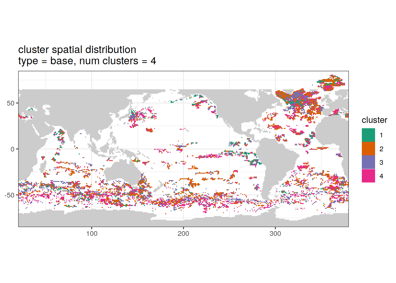
| Version | Author | Date |
|---|---|---|
| 7b7b3b3 | ds2n19 | 2023-12-18 |
[[2]]
| Version | Author | Date |
|---|---|---|
| 7b7b3b3 | ds2n19 | 2023-12-18 |
Adjusted profiles
if (opt_norm_anomaly) {

  # create figure
  anomaly_cluster_all %>%
    filter (profile_type == "adjusted") %>%
    group_split(profile_type, num_clusters) %>%
    map(
      ~ map +
        geom_tile(data = .x,
                  aes(
                    x = lon,
                    y = lat,
                    fill = cluster
                  )) +
        lims(y = opt_map_lat_limit) +
        scale_fill_brewer(palette = 'Dark2') +
        labs(
          title = paste0(
            'cluster spatial distribution \n',
            'type = ', unique(.x$profile_type), ', ',
            'num clusters = ', unique(.x$num_clusters)
          ),
        )
    )

}
[[1]]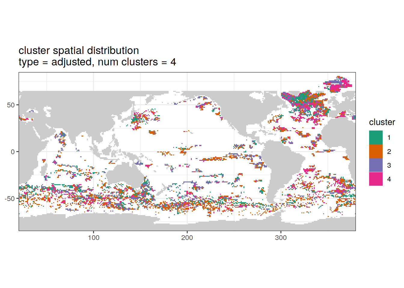
| Version | Author | Date |
|---|---|---|
| 7b7b3b3 | ds2n19 | 2023-12-18 |
[[2]]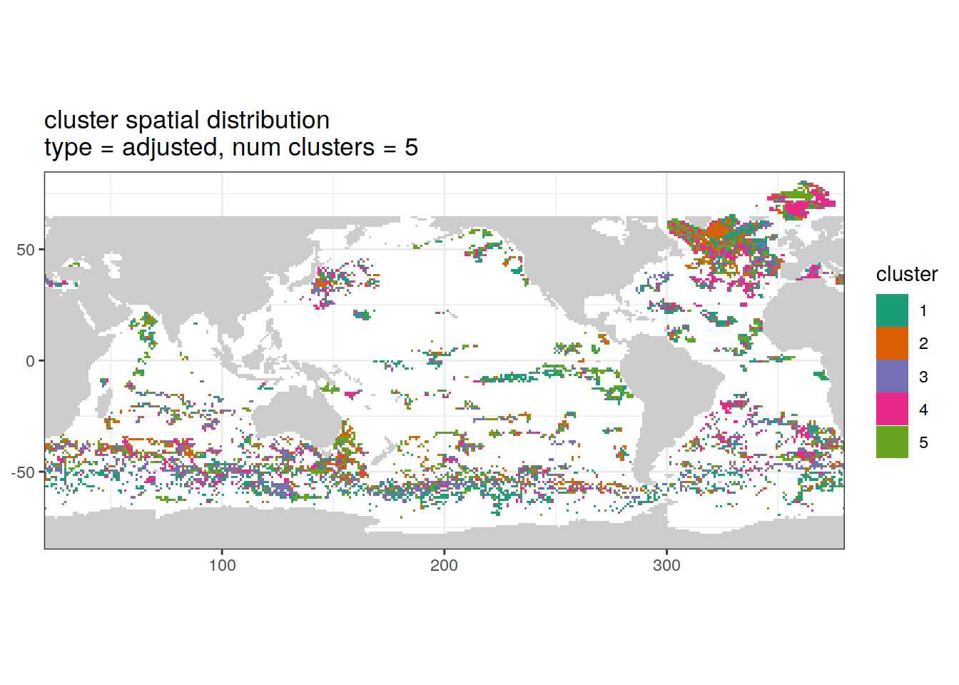
| Version | Author | Date |
|---|---|---|
| 7b7b3b3 | ds2n19 | 2023-12-18 |
Cluster spatial counts
count of measurements for each cluster on separate maps, spatial analysis
# Count profiles
cluster_by_location <- anomaly_cluster_all %>%
  count(profile_type, num_clusters, file_id, lat, lon, cluster,
        name = "count_cluster")

# # Add cluster counts to
cluster_by_location <- left_join(cluster_by_location, cluster_count)

# create figure
cluster_by_location %>%
  filter (profile_type == "base") %>%
  group_split(profile_type, num_clusters) %>%
  map(
    ~ map +
      geom_tile(data = .x %>%
                  count(lat, lon, cluster, count_profiles),
                aes(
                  x = lon,
                  y = lat,
                  fill = n
                )) +
      lims(y = opt_map_lat_limit) +
      scale_fill_gradient(low = "blue",
                          high = "red",
                          trans = "log10") +
      facet_wrap(~ paste0(cluster, " (", formatC(count_profiles, big.mark=",") , ")"), ncol = 2) +
      labs(
        title = paste0(
          'cluster spatial distribution \n',
          'type = ', unique(.x$profile_type), ', ',
          'num clusters = ', unique(.x$num_clusters)
        )
      )
  )
[[1]]
| Version | Author | Date |
|---|---|---|
| 7b7b3b3 | ds2n19 | 2023-12-18 |
[[2]]
| Version | Author | Date |
|---|---|---|
| 7b7b3b3 | ds2n19 | 2023-12-18 |
Adjusted profiles
if (opt_norm_anomaly) {

  # create figure
  cluster_by_location %>%
    filter (profile_type == "adjusted") %>%
    group_split(profile_type, num_clusters) %>%
    map(
      ~ map +
        geom_tile(data = .x %>%
                    count(lat, lon, cluster, count_profiles),
                  aes(
                    x = lon,
                    y = lat,
                    fill = n
                  )) +
        lims(y = opt_map_lat_limit) +
        scale_fill_gradient(low = "blue",
                            high = "red",
                            trans = "log10") +
        facet_wrap(~ paste0(cluster, " (", formatC(count_profiles, big.mark=",") , ")"), ncol = 2) +
        labs(
          title = paste0(
            'cluster spatial distribution \n',
            'type = ', unique(.x$profile_type), ', ',
            'num clusters = ', unique(.x$num_clusters)
          )
        )
    )

}
[[1]]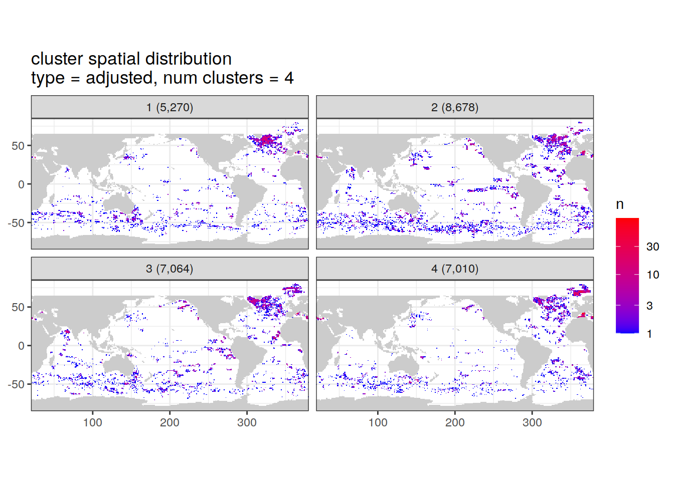
| Version | Author | Date |
|---|---|---|
| 7b7b3b3 | ds2n19 | 2023-12-18 |
[[2]]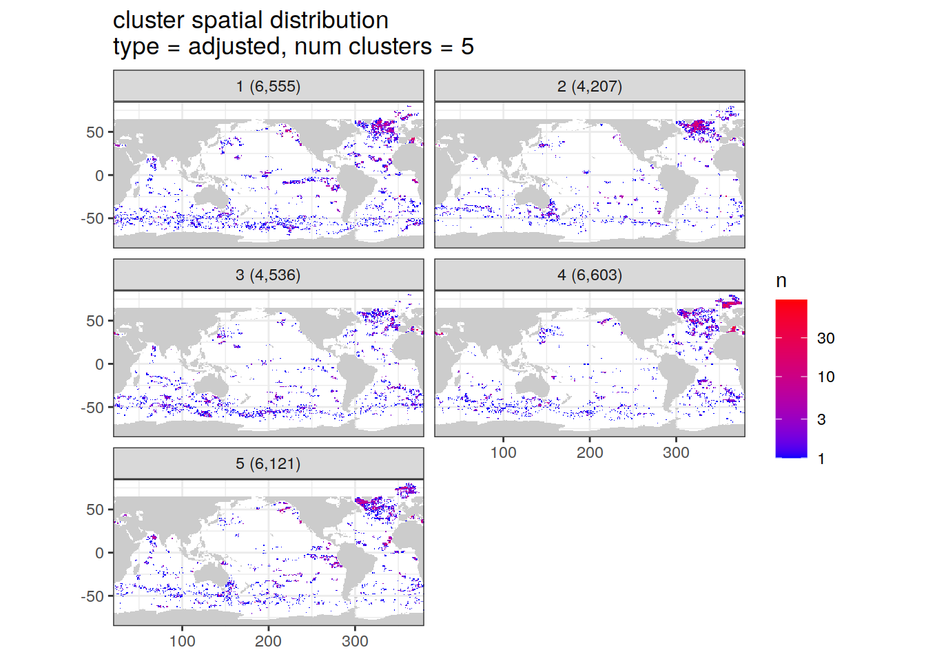
| Version | Author | Date |
|---|---|---|
| 7b7b3b3 | ds2n19 | 2023-12-18 |
sessionInfo()R version 4.2.2 (2022-10-31)
Platform: x86_64-pc-linux-gnu (64-bit)
Running under: openSUSE Leap 15.5
Matrix products: default
BLAS: /usr/local/R-4.2.2/lib64/R/lib/libRblas.so
LAPACK: /usr/local/R-4.2.2/lib64/R/lib/libRlapack.so
locale:
[1] LC_CTYPE=en_US.UTF-8 LC_NUMERIC=C
[3] LC_TIME=en_US.UTF-8 LC_COLLATE=en_US.UTF-8
[5] LC_MONETARY=en_US.UTF-8 LC_MESSAGES=en_US.UTF-8
[7] LC_PAPER=en_US.UTF-8 LC_NAME=C
[9] LC_ADDRESS=C LC_TELEPHONE=C
[11] LC_MEASUREMENT=en_US.UTF-8 LC_IDENTIFICATION=C
attached base packages:
[1] stats graphics grDevices utils datasets methods base
other attached packages:
[1] yardstick_1.2.0 workflowsets_1.0.1 workflows_1.1.3 tune_1.1.2
[5] rsample_1.2.0 recipes_1.0.8 parsnip_1.1.1 modeldata_1.2.0
[9] infer_1.0.5 dials_1.2.0 scales_1.2.1 broom_1.0.5
[13] tidymodels_1.1.1 ggpmisc_0.5.4-1 ggpp_0.5.5 ggforce_0.4.1
[17] gsw_1.1-1 gridExtra_2.3 lubridate_1.9.0 timechange_0.1.1
[21] argodata_0.1.0 forcats_0.5.2 stringr_1.5.0 dplyr_1.1.3
[25] purrr_1.0.2 readr_2.1.3 tidyr_1.3.0 tibble_3.2.1
[29] ggplot2_3.4.4 tidyverse_1.3.2
loaded via a namespace (and not attached):
[1] googledrive_2.0.0 colorspace_2.0-3 ellipsis_0.3.2
[4] class_7.3-20 rprojroot_2.0.3 fs_1.5.2
[7] rstudioapi_0.15.0 furrr_0.3.1 listenv_0.8.0
[10] farver_2.1.1 MatrixModels_0.5-1 prodlim_2019.11.13
[13] fansi_1.0.3 xml2_1.3.3 codetools_0.2-18
[16] splines_4.2.2 cachem_1.0.6 knitr_1.41
[19] polyclip_1.10-4 polynom_1.4-1 jsonlite_1.8.3
[22] workflowr_1.7.0 dbplyr_2.2.1 compiler_4.2.2
[25] httr_1.4.4 backports_1.4.1 assertthat_0.2.1
[28] Matrix_1.5-3 fastmap_1.1.0 gargle_1.2.1
[31] cli_3.6.1 later_1.3.0 tweenr_2.0.2
[34] htmltools_0.5.3 quantreg_5.94 tools_4.2.2
[37] gtable_0.3.1 glue_1.6.2 Rcpp_1.0.10
[40] cellranger_1.1.0 jquerylib_0.1.4 RNetCDF_2.6-1
[43] DiceDesign_1.9 vctrs_0.6.4 iterators_1.0.14
[46] timeDate_4021.106 xfun_0.35 gower_1.0.0
[49] globals_0.16.2 rvest_1.0.3 lifecycle_1.0.3
[52] googlesheets4_1.0.1 future_1.29.0 MASS_7.3-58.1
[55] ipred_0.9-13 hms_1.1.2 promises_1.2.0.1
[58] parallel_4.2.2 SparseM_1.81 RColorBrewer_1.1-3
[61] yaml_2.3.6 sass_0.4.4 rpart_4.1.19
[64] stringi_1.7.8 highr_0.9 foreach_1.5.2
[67] lhs_1.1.6 hardhat_1.3.0 lava_1.7.0
[70] rlang_1.1.1 pkgconfig_2.0.3 evaluate_0.18
[73] lattice_0.20-45 labeling_0.4.2 tidyselect_1.2.0
[76] here_1.0.1 parallelly_1.32.1 magrittr_2.0.3
[79] R6_2.5.1 generics_0.1.3 DBI_1.1.3
[82] pillar_1.9.0 haven_2.5.1 whisker_0.4
[85] withr_2.5.0 survival_3.4-0 nnet_7.3-18
[88] future.apply_1.10.0 modelr_0.1.10 crayon_1.5.2
[91] utf8_1.2.2 tzdb_0.3.0 rmarkdown_2.18
[94] grid_4.2.2 readxl_1.4.1 git2r_0.30.1
[97] reprex_2.0.2 digest_0.6.30 httpuv_1.6.6
[100] GPfit_1.0-8 munsell_0.5.0 viridisLite_0.4.1
[103] bslib_0.4.1