Comparison between Argo and CESM
Marguerite Larriere & Jens Daniel Müller
15 May, 2024
Last updated: 2024-05-15
Checks: 7 0
Knit directory:
bgc_argo_r_argodata/analysis/
This reproducible R Markdown analysis was created with workflowr (version 1.7.0). The Checks tab describes the reproducibility checks that were applied when the results were created. The Past versions tab lists the development history.
Great! Since the R Markdown file has been committed to the Git repository, you know the exact version of the code that produced these results.
Great job! The global environment was empty. Objects defined in the global environment can affect the analysis in your R Markdown file in unknown ways. For reproduciblity it’s best to always run the code in an empty environment.
The command set.seed(20211008) was run prior to running
the code in the R Markdown file. Setting a seed ensures that any results
that rely on randomness, e.g. subsampling or permutations, are
reproducible.
Great job! Recording the operating system, R version, and package versions is critical for reproducibility.
Nice! There were no cached chunks for this analysis, so you can be confident that you successfully produced the results during this run.
Great job! Using relative paths to the files within your workflowr project makes it easier to run your code on other machines.
Great! You are using Git for version control. Tracking code development and connecting the code version to the results is critical for reproducibility.
The results in this page were generated with repository version bbf732b. See the Past versions tab to see a history of the changes made to the R Markdown and HTML files.
Note that you need to be careful to ensure that all relevant files for
the analysis have been committed to Git prior to generating the results
(you can use wflow_publish or
wflow_git_commit). workflowr only checks the R Markdown
file, but you know if there are other scripts or data files that it
depends on. Below is the status of the Git repository when the results
were generated:
Ignored files:
    Ignored:    .Rproj.user/

Untracked files:
    Untracked:  analysis/draft.Rmd
    Untracked:  load_argo_core_output.txt

Unstaged changes:
    Deleted:    analysis/MHWs_categorisation.Rmd
    Modified:   analysis/MHWs_vertical_anomaly.Rmd
    Modified:   analysis/_site.yml
    Modified:   analysis/anomaly_SST_2023.Rmd
    Modified:   analysis/child/cluster_analysis_base.Rmd
    Modified:   analysis/coverage_maps_North_Atlantic.Rmd
    Modified:   analysis/load_broullon_DIC_TA_clim.Rmd
    Modified:   code/Workflowr_project_managment.R
    Modified:   code/start_background_job.R
    Modified:   code/start_background_job_load.R
    Modified:   code/start_background_job_partial.R
Note that any generated files, e.g. HTML, png, CSS, etc., are not included in this status report because it is ok for generated content to have uncommitted changes.
These are the previous versions of the repository in which changes were
made to the R Markdown (analysis/CESM_comparison.Rmd) and
HTML (docs/CESM_comparison.html) files. If you’ve
configured a remote Git repository (see ?wflow_git_remote),
click on the hyperlinks in the table below to view the files as they
were in that past version.
| File | Version | Author | Date | Message |
|---|---|---|---|---|
| Rmd | bbf732b | mlarriere | 2024-05-15 | CESM climatology |
| html | 96d4b76 | mlarriere | 2024-05-14 | Build site. |
| Rmd | 91e6028 | mlarriere | 2024-05-13 | adding subsection CESM comparison |
| html | af6594f | mlarriere | 2024-05-13 | Build site. |
| Rmd | 30f9250 | mlarriere | 2024-05-13 | Adding CESM subsection |
Task
Dependencies
Outputs
path CESM 2023 data: “/nfs/kryo/work/loher/GlobalMarineHeatwaves/ETHZ_BEC/Heatwaves_RunA.nc” variable for temperature: thetao
path_emlr_utilities <- "/nfs/kryo/work/jenmueller/emlr_cant/utilities/files/"
path_basin_mask <- "/nfs/kryo/work/datasets/gridded/ocean/interior/reccap2/supplementary/"

path_argo_core <- '/nfs/kryo/work/datasets/ungridded/3d/ocean/floats/core_argo_r_argodata_2024-03-13'
path_argo_core_preprocessed <- paste0(path_argo_core, "/preprocessed_core_data")

path_CESM<-"/nfs/kryo/work/loher/GlobalMarineHeatwaves/ETHZ_BEC/"
Read data
# Read NetCDF file containing CESM outputs (35 variables - 4dim: time, lat, lon, depth)
CESM_temp <- tidync(paste0(path_CESM, "Heatwaves_RunA.nc"))
CESM_temp <- CESM_temp %>%
  hyper_tibble(select_var = "thetao", # thetao: seawater potential temperature [°C]
                       force = TRUE)

CESM_temp <- CESM_temp %>%
  filter(thetao < 1e36) %>% # thetao ~ e36 because??
  rename(temp = thetao)

gc()
used (Mb) gc trigger (Mb) max used (Mb)
Ncells 1995040 106.6 4035317 215.6 3470729 185.4
Vcells 5267718845 40189.6 21682694924 165425.9 26690135370 203629.6CESM_temp <- CESM_temp %>%
mutate(time = ymd_hms("1980-01-01 00:00:00") + days(time))
gc() used (Mb) gc trigger (Mb) max used (Mb)
Ncells 2004397 107.1 4035317 215.6 3470729 185.4
Vcells 5267740084 40189.7 24264805791 185125.8 28959495069 220943.5CESM_temp$year <- year(CESM_temp$time)
CESM_temp$month <- month(CESM_temp$time)
gc() used (Mb) gc trigger (Mb) max used (Mb)
Ncells 2004486 107.1 4035317 215.6 3470729 185.4
Vcells 7373672463 56256.7 24264805791 185125.8 28959495069 220943.5#Area of interest: North Atlantic east - lat:(0,40), lon:(-30,0)
CESM_temp <- CESM_temp %>%
mutate(lon = ifelse(lon > 180, lon - 360, lon))
CESM_natlantic_east <- CESM_temp %>%
filter(lat>0, lat<40, -30<lon, lon<0)
#Select 2023
CESM_natlantic_east_2023 <- CESM_natlantic_east %>%
filter(year==2023)
gc() used (Mb) gc trigger (Mb) max used (Mb)
Ncells 2004591 107.1 4035317 215.6 3470729 185.4
Vcells 7518163058 57359.1 24264805791 185125.8 28959495069 220943.5# rm(CESM_temp)# Visualization
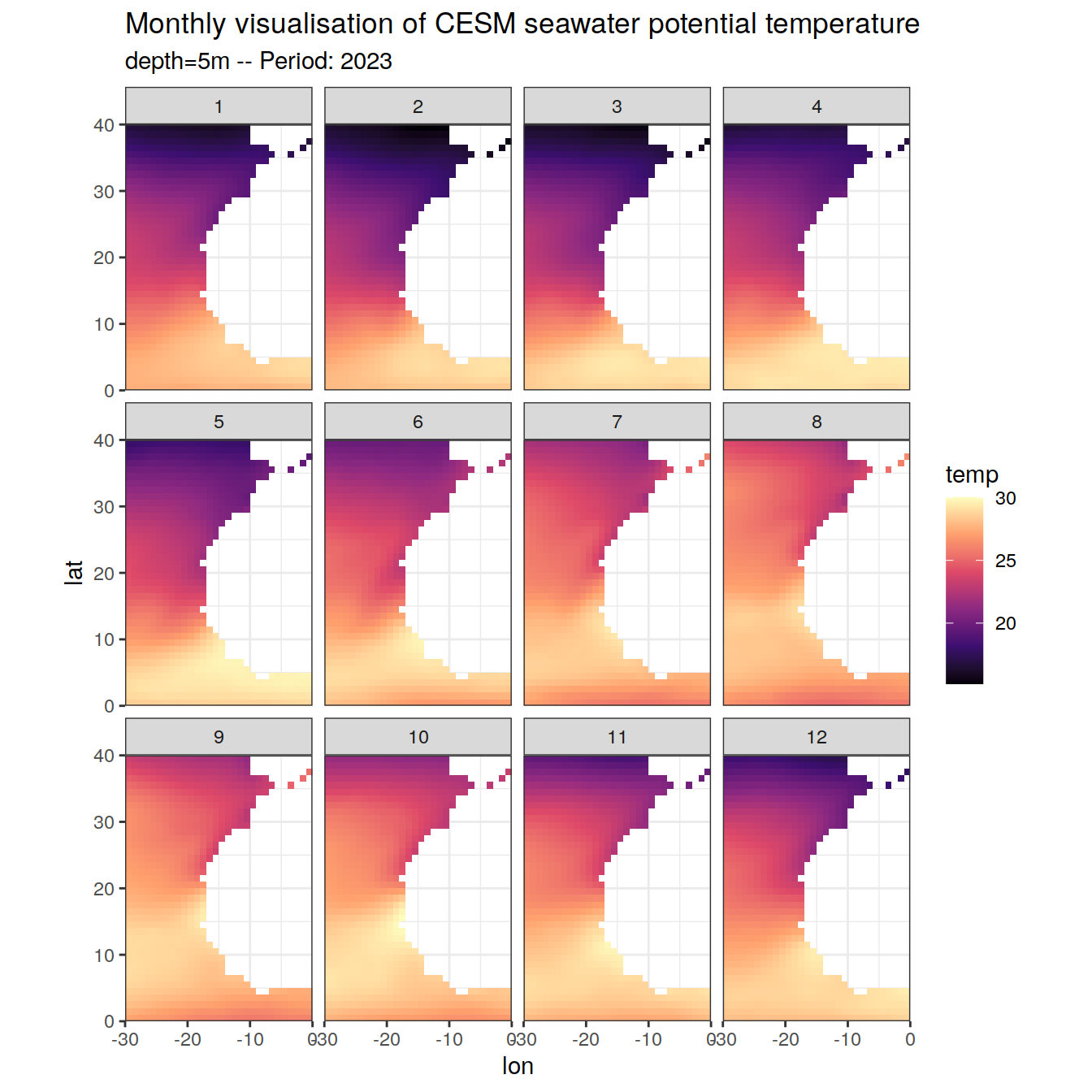
CESM_natlantic_east_2023 %>%
filter(depth == 5) %>%
ggplot(aes(lon, lat, fill = temp)) +
geom_raster() +
scale_fill_viridis_c(option = "magma") +
labs(title = "Monthly visualisation of CESM seawater potential temperature",
subtitle = paste0("depth=5m -- Period: 2023"))+
coord_quickmap(expand = 0)+
facet_wrap(~month, nrow = 3)
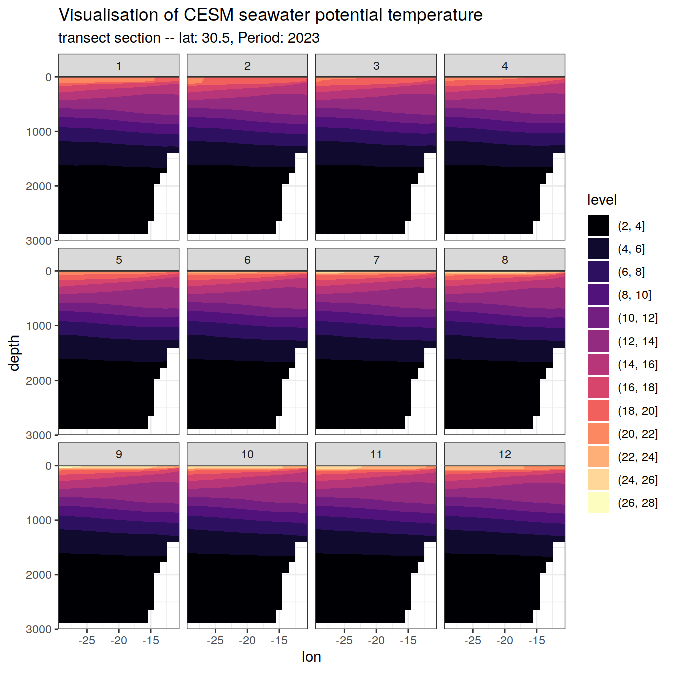
CESM_natlantic_east_2023 %>%
  filter(lat == 30.5) %>%
  ggplot(aes(lon, depth, z = temp)) +
  geom_contour_filled(breaks = seq(-10,40,2)) +
  scale_y_reverse(limits = c(3000, 0)) +
  coord_cartesian(expand = 0) +
  labs(title = "Visualisation of CESM seawater potential temperature",
       subtitle = paste0( "transect section -- lat: 30.5, Period: 2023"))+
  scale_fill_viridis_d(option = "magma")+
  facet_wrap(~month, nrow = 3)
#Climatology of CESM temp output over the period 2004-2019 (to match with argo climatology) -- only on the North Atlantic east
CESM_2004_2019_natlantic_east<- CESM_natlantic_east %>%
  filter(year>=2004, year<=2019)

CESM_2004_2019_natlantic_east<-CESM_2004_2019_natlantic_east %>%
  group_by(lat, lon, depth, month) %>%
  summarize(mean_temp=mean(temp, na.rm=TRUE))

# Visualization
CESM_2004_2019_natlantic_east %>%
  filter(depth == 5) %>%
  ggplot(aes(lon, lat, fill = mean_temp)) +
  geom_raster() +
  scale_fill_viridis_c(option = "magma") +
  labs(title = "Mean CESM seawater potential temperature",
       subtitle = paste0("depth=5m, Period: 2004-2019"))+
  coord_quickmap(expand = 0)+
  facet_wrap(~month, nrow = 3)
CESM_2004_2019_natlantic_east %>%
  filter(lat == 30.5) %>%
  ggplot(aes(lon, depth, z = mean_temp)) +
  geom_contour_filled(breaks = seq(-10,40,2)) +
  scale_y_reverse(limits = c(3000, 0)) +
  coord_cartesian(expand = 0) +
  labs(title = "Mean CESM seawater potential temperature",
       subtitle = paste0( "transect section -- lat: 30.5, Period: 2004-2019"))+
  scale_fill_viridis_d(option = "magma")+
  facet_wrap(~month, nrow = 3)
# Temperature anomaly
CESM_anomaly_natlantic_east_2023 <- inner_join(CESM_natlantic_east_2023, CESM_2004_2019_natlantic_east, by = c("month", "lat", "lon", "depth"))


# Calculate temperature anomaly
CESM_anomaly_natlantic_east_2023 <- CESM_anomaly_natlantic_east_2023 %>%
    mutate(temp_anomaly = temp - mean_temp)

#Write
write_rds(CESM_anomaly_natlantic_east_2023,
          file = paste0(path_argo_core_preprocessed,"/", "CESM_temp_anomaly2023_NorthAtlantic_east_clim2004-2019.rds"))

# rm(merged_data, CESM_2004_2019_natlantic_east)
gc()
used (Mb) gc trigger (Mb) max used (Mb)
Ncells 2428685 129.8 6548621 349.8 6548621 349.8
Vcells 7526086630 57419.5 24264805791 185125.8 28959495069 220943.5# Visualization
CESM_anomaly_natlantic_east_2023 %>%
filter(depth == 5) %>%
ggplot(aes(lon, lat, fill = temp_anomaly)) +
geom_raster() +
scale_fill_viridis_c(option = "magma") +
labs(title = "CESM temperature anomaly - 2023",
subtitle = paste0("depth=5m, clim: 2004-2019"))+
coord_quickmap(expand = 0)+
facet_wrap(~month, nrow = 3)
CESM_anomaly_natlantic_east_2023 %>%
  filter(lat == 30.5) %>%
  ggplot(aes(lon, depth, z = temp_anomaly)) +
  geom_contour_filled(breaks = seq(-10,40,0.5)) +
  scale_y_reverse(limits = c(3000, 0)) +
  coord_cartesian(expand = 0) +
  labs(title = "CESM temperature anomaly - 2023",
       subtitle = paste0( "transect section -- lat: 30.5, clim: 2004-2019"))+
  scale_fill_viridis_d(option = "magma")+
  facet_wrap(~month, nrow = 3)
sessionInfo()R version 4.2.2 (2022-10-31)
Platform: x86_64-pc-linux-gnu (64-bit)
Running under: openSUSE Leap 15.5
Matrix products: default
BLAS: /usr/local/R-4.2.2/lib64/R/lib/libRblas.so
LAPACK: /usr/local/R-4.2.2/lib64/R/lib/libRlapack.so
locale:
[1] LC_CTYPE=en_US.UTF-8 LC_NUMERIC=C
[3] LC_TIME=en_US.UTF-8 LC_COLLATE=en_US.UTF-8
[5] LC_MONETARY=en_US.UTF-8 LC_MESSAGES=en_US.UTF-8
[7] LC_PAPER=en_US.UTF-8 LC_NAME=C
[9] LC_ADDRESS=C LC_TELEPHONE=C
[11] LC_MEASUREMENT=en_US.UTF-8 LC_IDENTIFICATION=C
attached base packages:
[1] stats graphics grDevices utils datasets methods base
other attached packages:
[1] collapse_2.0.13 ncdf4_1.22 tidync_0.3.0 marelac_2.1.10
[5] shape_1.4.6 RColorBrewer_1.1-3 stars_0.6-0 sf_1.0-9
[9] abind_1.4-5 paletteer_1.6.0 cluster_2.1.6 gridExtra_2.3
[13] viridis_0.6.2 viridisLite_0.4.1 lubridate_1.9.0 timechange_0.1.1
[17] forcats_0.5.2 stringr_1.5.0 dplyr_1.1.3 purrr_1.0.2
[21] readr_2.1.3 tidyr_1.3.0 tibble_3.2.1 ggplot2_3.4.4
[25] tidyverse_1.3.2 workflowr_1.7.0
loaded via a namespace (and not attached):
[1] fs_1.5.2 gsw_1.1-1 httr_1.4.4
[4] rprojroot_2.0.3 tools_4.2.2 backports_1.4.1
[7] bslib_0.4.1 utf8_1.2.2 R6_2.5.1
[10] KernSmooth_2.23-20 DBI_1.2.2 colorspace_2.0-3
[13] withr_2.5.0 tidyselect_1.2.0 processx_3.8.0
[16] compiler_4.2.2 git2r_0.30.1 cli_3.6.1
[19] rvest_1.0.3 RNetCDF_2.6-1 xml2_1.3.3
[22] isoband_0.2.6 labeling_0.4.2 sass_0.4.4
[25] scales_1.2.1 classInt_0.4-8 SolveSAPHE_2.1.0
[28] callr_3.7.3 proxy_0.4-27 digest_0.6.30
[31] oce_1.7-10 rmarkdown_2.18 pkgconfig_2.0.3
[34] htmltools_0.5.8.1 highr_0.9 dbplyr_2.2.1
[37] fastmap_1.1.0 rlang_1.1.1 readxl_1.4.1
[40] rstudioapi_0.15.0 farver_2.1.1 jquerylib_0.1.4
[43] generics_0.1.3 jsonlite_1.8.3 googlesheets4_1.0.1
[46] magrittr_2.0.3 ncmeta_0.3.5 Rcpp_1.0.10
[49] munsell_0.5.0 fansi_1.0.3 lifecycle_1.0.3
[52] stringi_1.7.8 whisker_0.4 yaml_2.3.6
[55] grid_4.2.2 parallel_4.2.2 promises_1.2.0.1
[58] crayon_1.5.2 haven_2.5.1 seacarb_3.3.1
[61] hms_1.1.2 knitr_1.41 ps_1.7.2
[64] pillar_1.9.0 reprex_2.0.2 glue_1.6.2
[67] evaluate_0.18 getPass_0.2-2 modelr_0.1.10
[70] vctrs_0.6.4 tzdb_0.3.0 httpuv_1.6.6
[73] cellranger_1.1.0 gtable_0.3.1 rematch2_2.1.2
[76] assertthat_0.2.1 cachem_1.0.6 xfun_0.35
[79] lwgeom_0.2-10 broom_1.0.5 e1071_1.7-12
[82] later_1.3.0 class_7.3-20 googledrive_2.0.0
[85] gargle_1.2.1 units_0.8-0 ellipsis_0.3.2