Extreme pH Profiles
Pasqualina Vonlanthen & Jens Daniel Müller
25 January, 2022
Last updated: 2022-01-25
Checks: 7 0
Knit directory: bgc_argo_r_argodata/
This reproducible R Markdown analysis was created with workflowr (version 1.7.0). The Checks tab describes the reproducibility checks that were applied when the results were created. The Past versions tab lists the development history.
Great! Since the R Markdown file has been committed to the Git repository, you know the exact version of the code that produced these results.
Great job! The global environment was empty. Objects defined in the global environment can affect the analysis in your R Markdown file in unknown ways. For reproduciblity it’s best to always run the code in an empty environment.
The command set.seed(20211008) was run prior to running the code in the R Markdown file. Setting a seed ensures that any results that rely on randomness, e.g. subsampling or permutations, are reproducible.
Great job! Recording the operating system, R version, and package versions is critical for reproducibility.
Nice! There were no cached chunks for this analysis, so you can be confident that you successfully produced the results during this run.
Great job! Using relative paths to the files within your workflowr project makes it easier to run your code on other machines.
Great! You are using Git for version control. Tracking code development and connecting the code version to the results is critical for reproducibility.
The results in this page were generated with repository version 3851824. See the Past versions tab to see a history of the changes made to the R Markdown and HTML files.
Note that you need to be careful to ensure that all relevant files for the analysis have been committed to Git prior to generating the results (you can use wflow_publish or wflow_git_commit). workflowr only checks the R Markdown file, but you know if there are other scripts or data files that it depends on. Below is the status of the Git repository when the results were generated:
Ignored files:
    Ignored:    .RData
    Ignored:    .Rhistory
    Ignored:    .Rproj.user/
    Ignored:    output/

Untracked files:
    Untracked:  code/OceanSODA_argo_extremes.R
    Untracked:  code/creating_dataframe.R
    Untracked:  code/creating_map.R
    Untracked:  code/merging_oceanSODA_Argo.R
    Untracked:  code/pH_data_timeseries.R
Note that any generated files, e.g. HTML, png, CSS, etc., are not included in this status report because it is ok for generated content to have uncommitted changes.
These are the previous versions of the repository in which changes were made to the R Markdown (analysis/extreme_pH.Rmd) and HTML (docs/extreme_pH.html) files. If you’ve configured a remote Git repository (see ?wflow_git_remote), click on the hyperlinks in the table below to view the files as they were in that past version.
| File | Version | Author | Date | Message |
|---|---|---|---|---|
| Rmd | 3851824 | pasqualina-vonlanthendinenna | 2022-01-25 | added basin-mean profiles |
| html | 962cdb9 | pasqualina-vonlanthendinenna | 2022-01-25 | Build site. |
| Rmd | 825a50a | pasqualina-vonlanthendinenna | 2022-01-25 | added seasonal and biome profiles |
| html | 3ae43e4 | pasqualina-vonlanthendinenna | 2022-01-24 | Build site. |
| Rmd | 3f8e824 | pasqualina-vonlanthendinenna | 2022-01-24 | updated 24/01 |
| html | 6b22341 | pasqualina-vonlanthendinenna | 2022-01-21 | Build site. |
| Rmd | e72d7ca | pasqualina-vonlanthendinenna | 2022-01-21 | updated linear regression to monthly |
| html | 587755e | pasqualina-vonlanthendinenna | 2022-01-21 | Build site. |
| Rmd | 7a9209b | pasqualina-vonlanthendinenna | 2022-01-21 | updated threshold calculation 2 |
| html | c96ad5e | pasqualina-vonlanthendinenna | 2022-01-21 | Build site. |
| Rmd | 58b3b3b | pasqualina-vonlanthendinenna | 2022-01-21 | updated threshold calculation |
| html | ed3fef2 | jens-daniel-mueller | 2022-01-07 | Build site. |
| Rmd | 3d2f8fc | jens-daniel-mueller | 2022-01-07 | code review |
| html | 486c9c8 | jens-daniel-mueller | 2022-01-07 | Build site. |
| Rmd | e9ad067 | jens-daniel-mueller | 2022-01-07 | code review |
| html | 343689f | pasqualina-vonlanthendinenna | 2022-01-06 | Build site. |
| Rmd | f53cc2d | pasqualina-vonlanthendinenna | 2022-01-06 | updated profile page |
| html | b8a6482 | pasqualina-vonlanthendinenna | 2022-01-03 | Build site. |
| Rmd | 054f8a6 | pasqualina-vonlanthendinenna | 2022-01-03 | added Argo profiles |
Task
Compare depth profiles of normal pH and of extreme pH, as identified in the surface OceanSODA pH data product
theme_set(theme_bw())
HNL_colors <- c("H" = "#b2182b",
                "N" = "#636363",
                "L" = "#2166ac")
Load data
path_argo <- '/nfs/kryo/work/updata/bgc_argo_r_argodata'
path_argo_preprocessed <- paste0(path_argo, "/preprocessed_bgc_data")
path_emlr_utilities <- "/nfs/kryo/work/jenmueller/emlr_cant/utilities/files/"
# RECCAP2-ocean region mask
region_masks_all_2x2 <- read_rds(file = paste0(path_argo_preprocessed,
"/region_masks_all_2x2.rds"))
region_masks_all_2x2 <- region_masks_all_2x2 %>%
rename(biome = value) %>%
filter(region == 'southern',
biome != 0) %>%
select(-region) %>%
mutate(coast = as.character(coast))
# WOA 18 basin mask
basinmask <-
read_csv(
paste(path_emlr_utilities,
"basin_mask_WOA18.csv",
sep = ""),
col_types = cols("MLR_basins" = col_character())
)
basinmask_2x2 <- basinmask %>%
filter(MLR_basins == unique(basinmask$MLR_basins)[1]) %>%
select(lon, lat, basin_AIP) %>%
mutate(
lat = cut(lat, seq(-90, 90, 2), seq(-89, 89, 2)),
lat = as.numeric(as.character(lat)),
lon = cut(lon, seq(20, 380, 2), seq(21, 379, 2)),
lon = as.numeric(as.character(lon))
) # regrid into 2x2º grid
# OceanSODA
OceanSODA <- read_rds(file = paste0(path_argo_preprocessed, "/OceanSODA.rds"))
OceanSODA <- OceanSODA %>%
mutate(month = month(date))
OceanSODA_2x2 <- OceanSODA %>%
mutate(
lat = cut(lat, seq(-90, 90, 2), seq(-89, 89, 2)),
lat = as.numeric(as.character(lat)),
lon = cut(lon, seq(20, 380, 2), seq(21, 379, 2)),
lon = as.numeric(as.character(lon))) # regrid into 2x2º grid
# group_by(lon, lat, date, year, month) %>%
# summarise(ph_month = mean(ph_total, na.rm = TRUE)) %>%
# ungroup()
# calculate mean pH for each 2x2 grid at each date
# load in the full argo data
full_argo <- read_rds(file = paste0(path_argo_preprocessed, "/bgc_merge_pH_qc_1.rds"))
# change the date format for compatibility with OceanSODA pH data
full_argo_2x2 <- full_argo %>%
mutate(year = year(date),
month = month(date)) %>%
mutate(date = ymd(format(date, "%Y-%m-15"))) %>%
mutate(
lat = cut(lat, seq(-90, 90, 2), seq(-89, 89, 2)),
lat = as.numeric(as.character(lat)),
lon = cut(lon, seq(20, 380, 2), seq(21, 379, 2)),
lon = as.numeric(as.character(lon))) # re-grid to 2x2
# group_by(lon, lat, date, year, month, depth, platform_number, cycle_number) %>%
# summarise(ph_adjusted_month = mean(ph_in_situ_total_adjusted, na.rm = TRUE),
# temp_adjusted_month = mean(temp_adjusted, na.rm = TRUE)) %>%
# ungroup()
# calculate mean pH and temperature for each 2x2 grid for each dateRegions
Biomes
basemap(limits = -32) +
  geom_spatial_tile(
    data = region_masks_all_2x2,
    aes(x = lon,
        y = lat,
        fill = biome),
    col = 'transparent'
  ) +
  scale_fill_brewer(palette = "Dark2")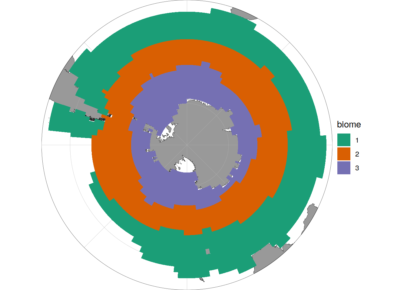
Coast
basemap(limits = -32) +
  geom_spatial_tile(
    data = region_masks_all_2x2,
    aes(x = lon,
        y = lat,
        fill = coast),
    col = 'transparent'
  ) +
  scale_fill_brewer(palette = "Dark2")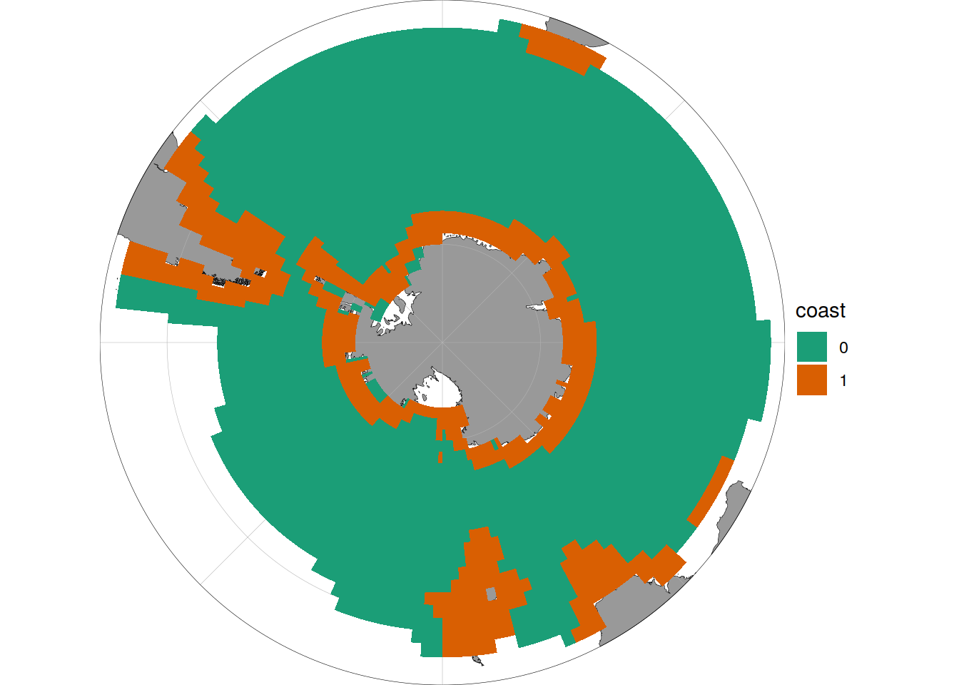
Apply region masks
region_masks_all_2x2 <- region_masks_all_2x2 %>%
  filter(coast == "0")
# keep only Southern Ocean data
OceanSODA_2x2_SO <- inner_join(OceanSODA_2x2, region_masks_all_2x2)
# add in basin separations
OceanSODA_2x2_SO <- inner_join(OceanSODA_2x2_SO, basinmask_2x2)
# (adds in duplicate rows?
# OceanSODA_2x2 -> 4234672 rows
# OceanSODA_2x2_SO -> 13988280 rows)
# remove the duplicate rows created by inner_join
OceanSODA_2x2_SO <- OceanSODA_2x2_SO %>%
distinct()
# (results in 988956 rows)
# keep only Southern Ocean argo data
full_argo_2x2_SO <- inner_join(full_argo_2x2, region_masks_all_2x2)
# add in basin separations
full_argo_2x2_SO <- inner_join(full_argo_2x2_SO, basinmask_2x2)
# remove duplicate rows (keep only distinct rows)
full_argo_2x2_SO <- full_argo_2x2_SO %>%
distinct()OceanSODA pH anomalies
Grid level
Climatological thresholds
Climatological monthly OceanSODA pH and the 5th and 95th percentiles, calculated for 2013-2021, with the full spatial OceanSODA data
# fit a linear regression of OceanSODA pH against time (temporal trend) in each lat/lon grid
OceanSODA_regression <- OceanSODA_2x2_SO %>%
  drop_na() %>%
  nest(data = -c(lon, lat, month)) %>%   # group by lon, lat
  mutate(fit = map(.x = data,
                   .f = ~ lm(ph_total ~ date, data = .x)),
         tidied = map(.x = fit, .f = tidy),
         augmented = map(.x = fit, .f = augment))

OceanSODA_regression <- OceanSODA_regression %>%
  unnest(tidied) %>%
  unnest(augmented)
# join the regression estimates to OceanSODA and remove duplicate rows
OceanSODA_2x2_SO_extreme_grid <- inner_join(OceanSODA_2x2_SO, OceanSODA_regression) %>%
distinct()
# sigma is the residual standard deviation
# .fitted are the predicted pH values by the linear model
# calculate H and L pH thresholds for climatological monthly pH
OceanSODA_2x2_SO_extreme_grid <- OceanSODA_2x2_SO_extreme_grid %>%
mutate(ph_L = .fitted - 2*(.sigma),
ph_H = .fitted + 2*(.sigma))# calculate climatological average OceanSODA pH
# and the 95th percentile of the monthly OceanSODA pH
#
# OceanSODA_2x2_SO_clim_grid <- OceanSODA_2x2_SO %>%
# group_by(lon, lat, month) %>%
# summarise(
# ph_N = mean(ph_total, na.rm = TRUE),
# ph_H = quantile(ph_total, 0.95, na.rm = TRUE),
# ph_L = quantile(ph_total, 0.05, na.rm = TRUE)
# ) %>%
# ungroup()
#
# OceanSODA_2x2_SO_extreme_grid <- inner_join(OceanSODA_2x2_SO, OceanSODA_2x2_SO_clim_grid)Anomaly identification
Calculate OceanSODA pH anomalies: L for abnormally low, H for abnormally high, N for normal pH
# when the in-situ OceanSODA pH is lower than the 5th percentile (predicted - 2*residual.st.dev), assign 'L' for low extreme
# when the in-situ OceanSODA pH exceeds the 95th percentile (predicted + 2*residual.st.dev), assign 'H' for high extreme
# when the in-situ OceanSODA pH is within 95% of the range, then assign 'N' for normal pH

OceanSODA_2x2_SO_extreme_grid <- OceanSODA_2x2_SO_extreme_grid %>%
  mutate(
    ph_extreme = case_when(
      ph_total < ph_L ~ 'L',
      ph_total > ph_H ~ 'H',
      TRUE ~ 'N'
    )
  ) %>%
  drop_na()

OceanSODA_2x2_SO_extreme_grid <- OceanSODA_2x2_SO_extreme_grid %>%
  mutate(ph_extreme = fct_relevel(ph_extreme, "H", "N", "L"))

# pivot_wider two columns (slope and intercept), values_from = estimate, names_from = terms, names.repair = 'unique'
# gives a slope and intercept column
# rename date...26 = slope and date...2 = date
OceanSODA_2x2_SO_extreme_grid <- OceanSODA_2x2_SO_extreme_grid %>%
  pivot_wider(names_from = term,
              values_from = estimate,
              names_repair = 'unique') %>%
  rename(date = date...2,
         regression_slope = date...26,
         regression_intercept = `(Intercept)`)

# fill in NAs in the slope and intercept columns (values from above for regression_slope and values from below for regression_intercept) (creates duplicate rows) and remove duplicate rows
# OceanSODA_2x2_SO_extreme_grid <- OceanSODA_2x2_SO_extreme_grid %>%
#   group_by(lon, lat, date, year, month) %>%
#   fill(regression_slope, .direction = 'up') %>%
#   fill(regression_intercept, .direction = 'down') %>%
#   distinct()
OceanSODA_2x2_SO_extreme_grid %>%
group_split(lon, lat, month) %>%
head(12) %>%
map(~ ggplot(data = .x) +
geom_point(aes(x = year,
y = ph_total,
col = ph_extreme)) +
geom_abline(data = .x, aes(slope = regression_slope,
intercept = regression_intercept - 2*.sigma),
linetype = 2) +
geom_abline(data = .x, aes(slope = regression_slope,
intercept = regression_intercept + 2*.sigma),
linetype = 2) +
geom_abline(data = .x, aes(intercept = regression_intercept,
slope = regression_slope)) +
labs(title = paste(fititle = paste(
"lon:", unique(.x$lon),
"| lat:", unique(.x$lat),
"| month:", unique(.x$month)
))) +
scale_color_manual(values = HNL_colors))[[1]]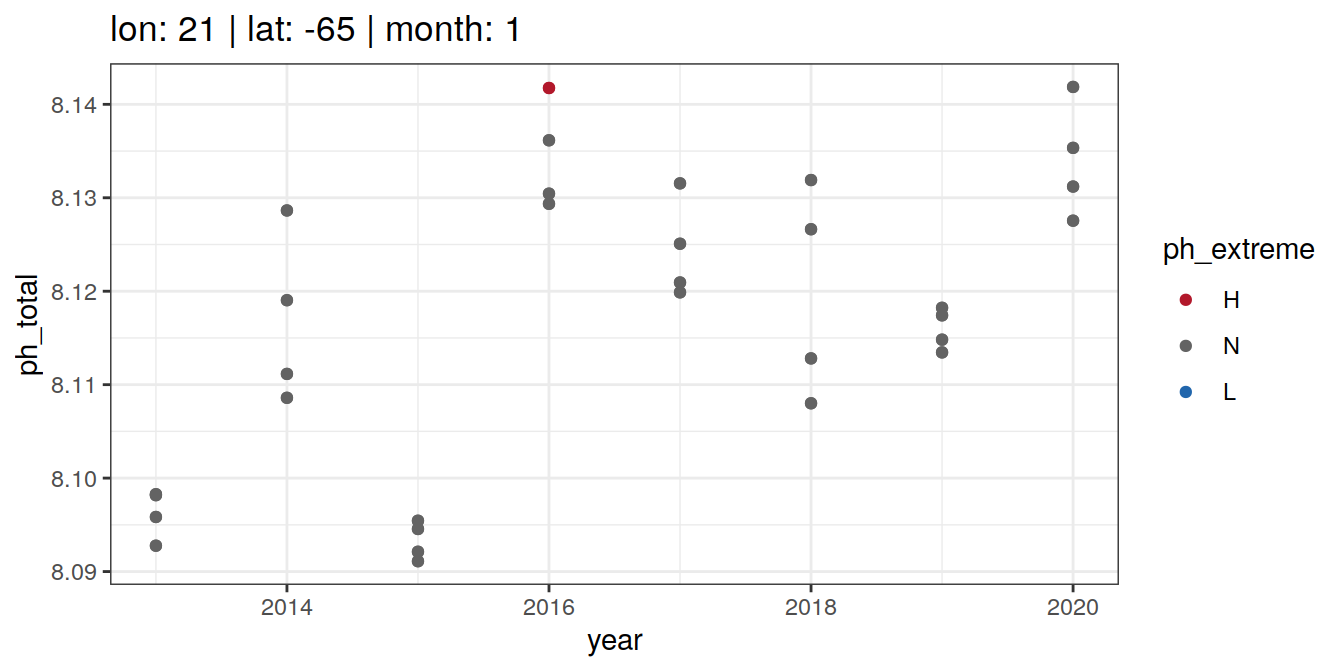
[[2]]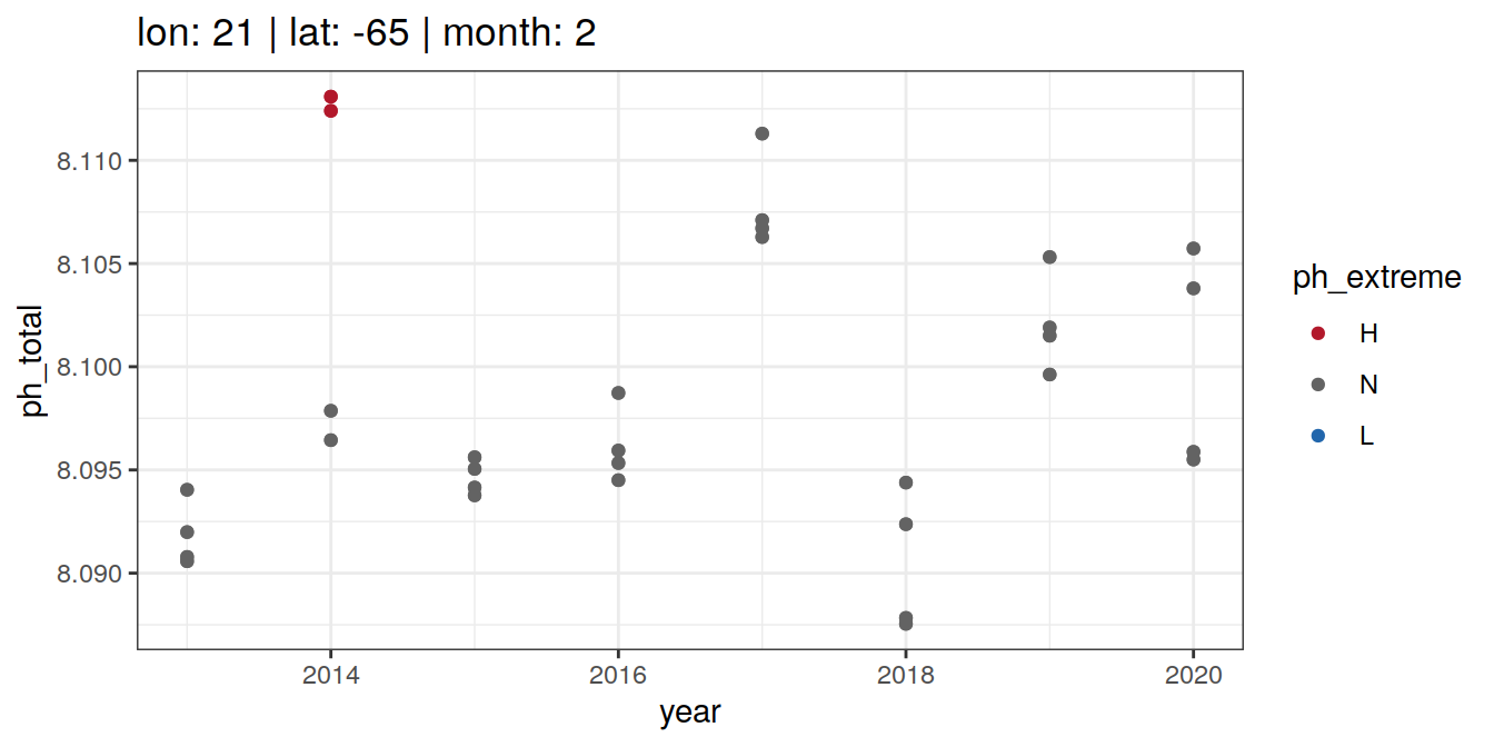
[[3]]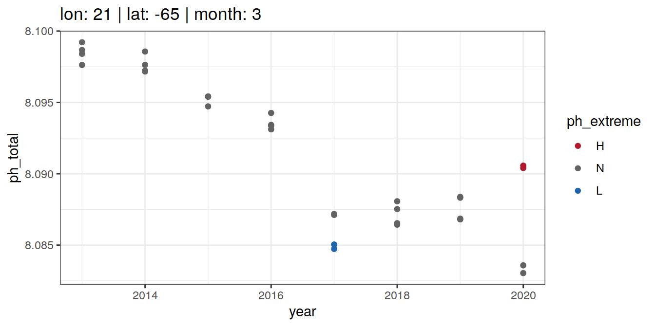
[[4]]
[[5]]
[[6]]
[[7]]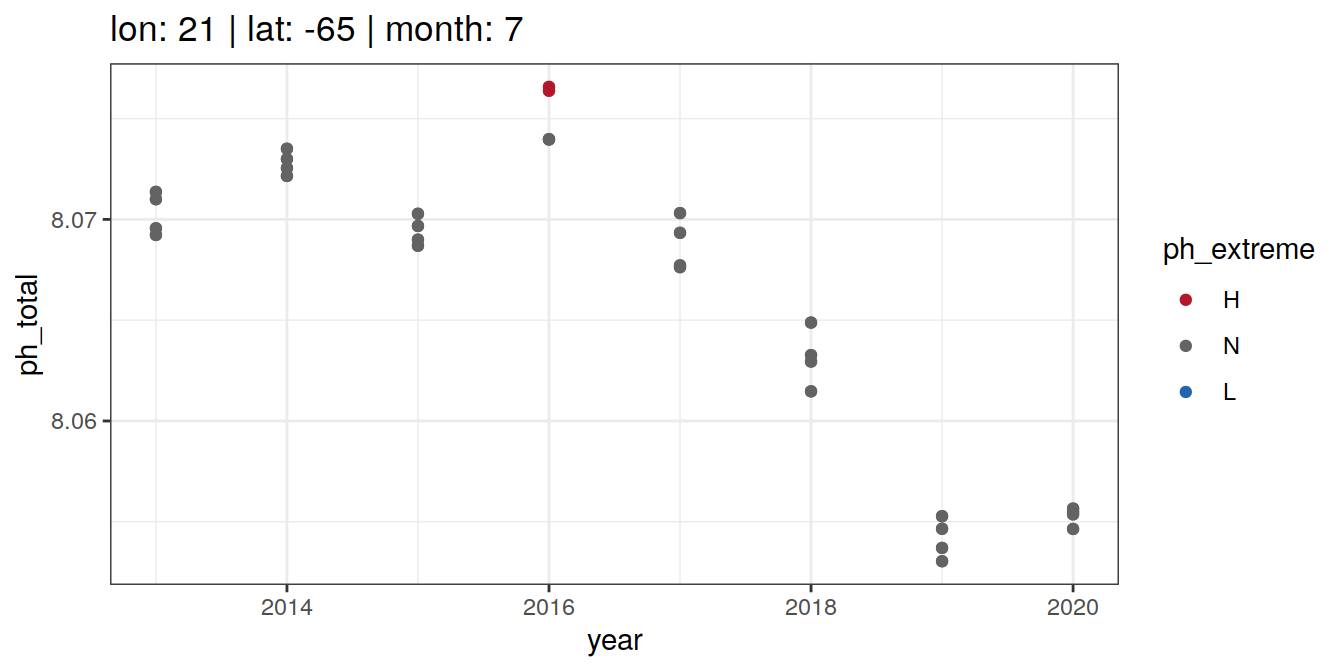
[[8]]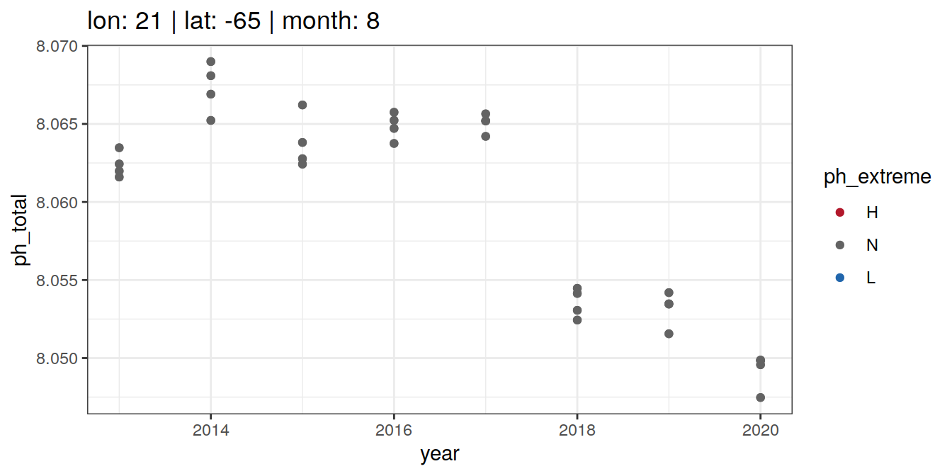
[[9]]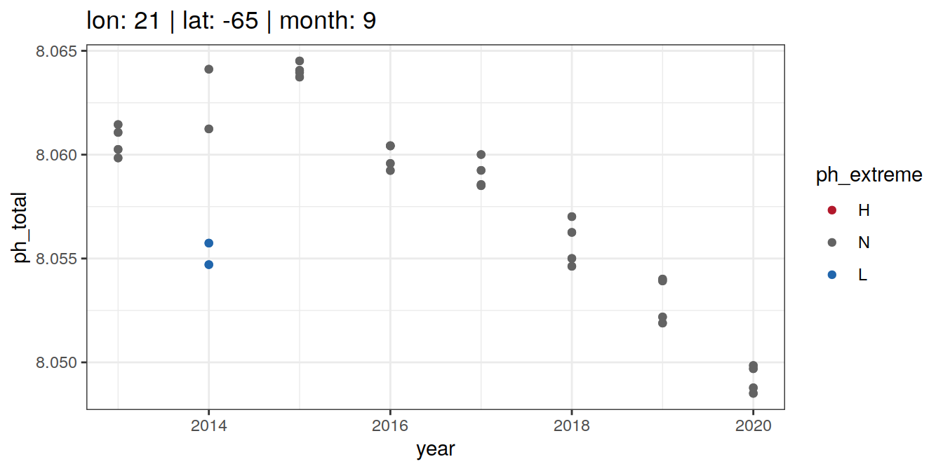
[[10]]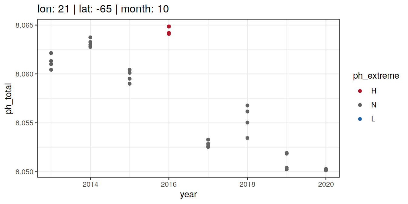
[[11]]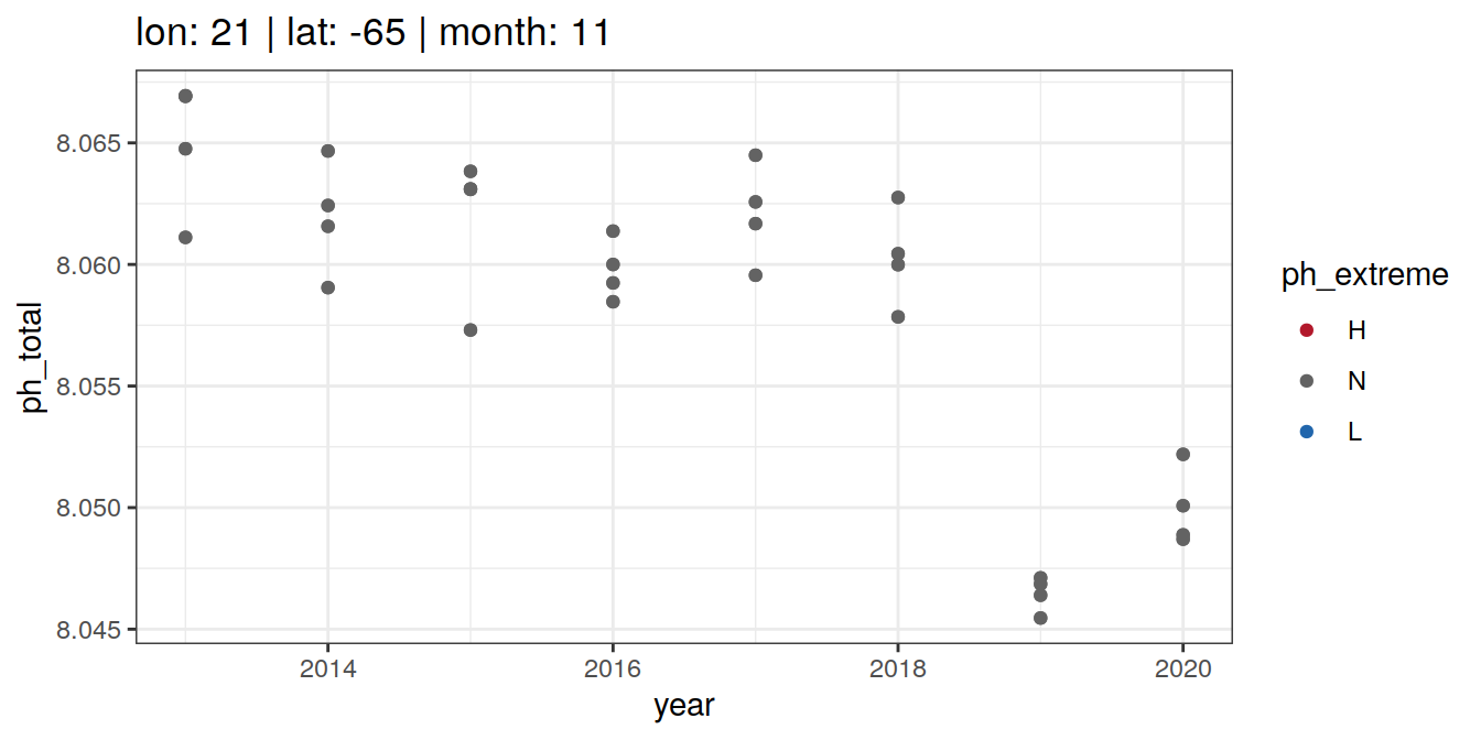
[[12]]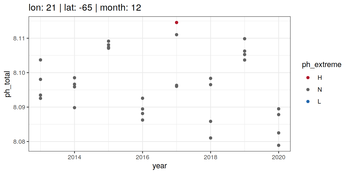
Anomaly maps
Location of OceanSODA pH extremes
OceanSODA_2x2_SO_extreme_grid %>%
  group_split(year) %>%
  #head(3) %>%
  map(
    ~ basemap(limits = -32, data = .x)+
      geom_spatial_tile(data = .x,
                        aes(x = lon,
                            y = lat,
                            fill = ph_extreme),
                        linejoin = 'mitre',
                        col = 'transparent',
                        detail = 60
                        ) +
      scale_fill_manual(values = HNL_colors) +
      facet_wrap(~month, ncol = 2)+
      labs(title = paste("Year:", unique(.x$year)),
           fill = 'pH')
  )
[[1]]
[[2]]
[[3]]
[[4]]
[[5]]
[[6]]
[[7]]
[[8]]
Anomaly time series
# calculate a regional mean pH for each biome, basin, and ph extreme (H/L/N) and plot a timeseries

OceanSODA_2x2_SO_extreme_grid %>%
  group_by(date, biome, basin_AIP, ph_extreme) %>%
  summarise(ph_regional = mean(ph_total, na.rm = TRUE)) %>%
  ungroup() %>%
  ggplot(aes(x = date, y = ph_regional, col = ph_extreme))+
  geom_point(size = 0.3)+
  geom_line()+
  scale_color_manual(values = HNL_colors) +
  facet_grid(basin_AIP~biome)+
  labs(x = 'date',
       y = 'regional mean pH',
       col = 'pH anomaly') +
  theme(legend.position = 'bottom')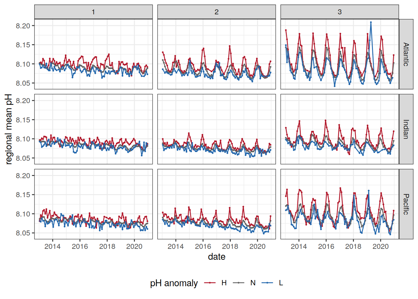
Anomaly histogram
OceanSODA_2x2_SO_extreme_grid %>%
  ggplot(aes(ph_total, col = ph_extreme)) +
  geom_density() +
  scale_color_manual(values = HNL_colors) +
  facet_grid(basin_AIP ~ biome) +
  coord_cartesian(xlim = c(8, 8.2)) +
  labs(x = 'value',
       y = 'density',
       col = 'pH anomaly') +
  theme(legend.position = 'bottom')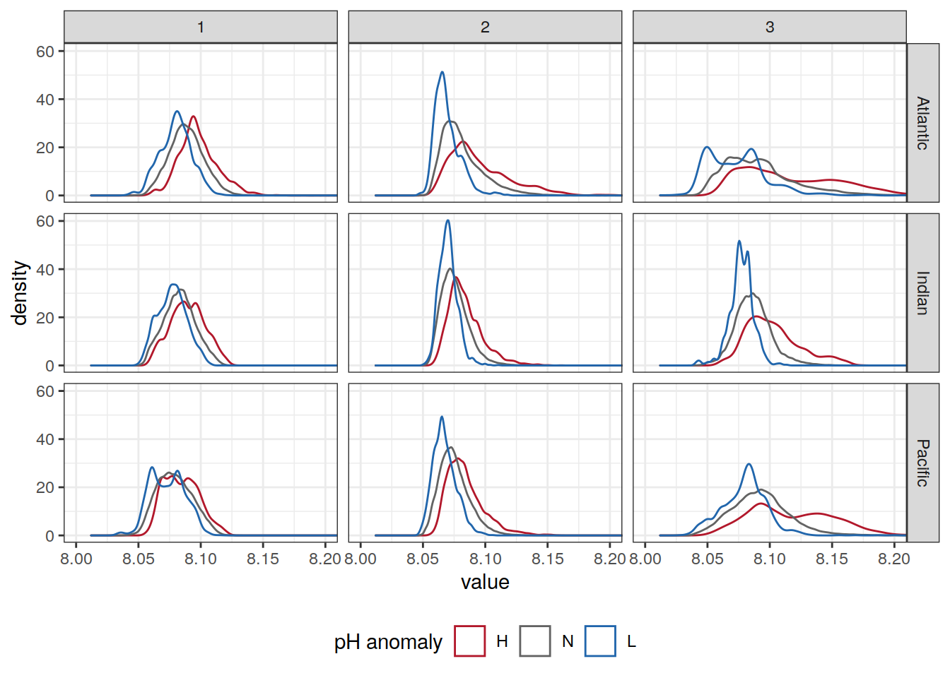
Threshold histogram
OceanSODA_2x2_SO_extreme_grid %>%
  mutate(ph_extreme = as.double(ph_extreme)) %>%
  pivot_longer(starts_with("ph_"),
               names_to = "level",
               values_to = "value",
               names_prefix = "ph_") %>%
  distinct() %>%
  ggplot(aes(value, col = level)) +
  geom_density() +
  scale_color_manual(values = HNL_colors, name = "threshold") +
  coord_cartesian(xlim = c(8, 8.2)) +
  lims(y = c(0, 230))+
  theme(legend.position = 'bottom')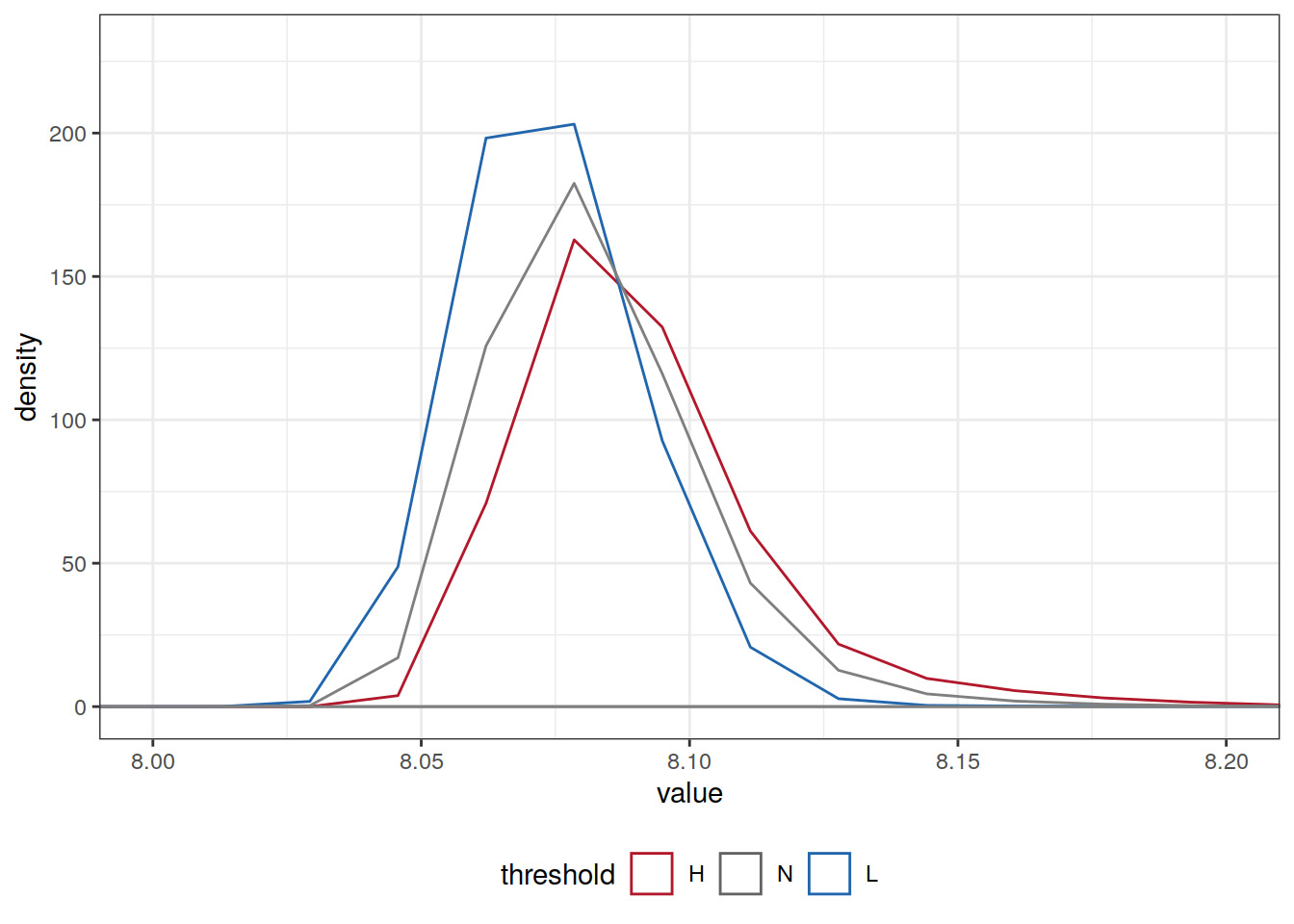
| Version | Author | Date |
|---|---|---|
| 962cdb9 | pasqualina-vonlanthendinenna | 2022-01-25 |
| 3ae43e4 | pasqualina-vonlanthendinenna | 2022-01-24 |
| 6b22341 | pasqualina-vonlanthendinenna | 2022-01-21 |
| 587755e | pasqualina-vonlanthendinenna | 2022-01-21 |
| c96ad5e | pasqualina-vonlanthendinenna | 2022-01-21 |
| ed3fef2 | jens-daniel-mueller | 2022-01-07 |
| 486c9c8 | jens-daniel-mueller | 2022-01-07 |
Biome level
Climatological thresholds
Climatological monthly OceanSODA pH and the 5th and 95th percentiles, calculated for 2013-2021, with the full spatial OceanSODA data
# calculate biome-mean pH for each date
OceanSODA_biome <- OceanSODA_2x2_SO %>%
  group_by(date, year, month, biome, basin_AIP) %>%
  summarise(biome_ph = mean(ph_total, na.rm = TRUE))
# fit a linear regression of biome-mean pH against time (temporal trend) in each biome/basin area
OceanSODA_biome_regression <- OceanSODA_biome %>%
drop_na() %>%
nest(data = -c(biome, basin_AIP, month)) %>% # group by biome, basin
mutate(fit = map(.x = data,
.f = ~ lm(biome_ph ~ date, data = .x)),
tidied = map(.x = fit, .f = tidy),
augmented = map(.x = fit, .f = augment))
OceanSODA_biome_regression <- OceanSODA_biome_regression %>%
unnest(tidied) %>%
unnest(augmented)# calculate climatological average OceanSODA pH
# and the 95th percentile of the monthly OceanSODA pH
# OceanSODA_2x2_SO_clim_biome <- OceanSODA_SO %>%
# group_by(biome, basin_AIP, month) %>%
# summarise(
# ph_N = mean(ph_total, na.rm = TRUE),
# ph_H = quantile(ph_total, 0.95, na.rm = TRUE),
# ph_L = quantile(ph_total, 0.05, na.rm = TRUE)
# ) %>%
# ungroup()
#
# OceanSODA_2x2_SO_extreme_biome <- inner_join(OceanSODA_SO, OceanSODA_2x2_SO_clim_biome)# join the regression estimates to OceanSODA and remove duplicate rows
OceanSODA_2x2_SO_extreme_biome <- inner_join(OceanSODA_2x2_SO, OceanSODA_biome_regression) %>%
distinct()
# sigma is the residual standard deviation
# .fitted are the predicted pH values by the linear model
# calculate H and L pH thresholds for climatological monthly pH
OceanSODA_2x2_SO_extreme_biome <- OceanSODA_2x2_SO_extreme_biome %>%
mutate(ph_L = .fitted - 2*(.sigma),
ph_H = .fitted + 2*(.sigma))Anomaly identification
Calculate OceanSODA pH anomalies: L for abnormally low, H for abnormally high, N for normal pH
# when the in-situ OceanSODA pH is lower than the 5th percentile, assign 'L' for low extreme
# when the in-situ OceanSODA pH exceeds the 95th percentile, assign 'H' for high extreme
# when the in-situ OceanSODA pH is within 95% of the range, then assign 'N' for normal pH
OceanSODA_2x2_SO_extreme_biome <- OceanSODA_2x2_SO_extreme_biome %>%
  mutate(
    ph_extreme = case_when(
      ph_total < ph_L ~ 'L',
      ph_total > ph_H ~ 'H',
      TRUE ~ 'N'
    )
  ) %>%
  drop_na()

OceanSODA_2x2_SO_extreme_biome <- OceanSODA_2x2_SO_extreme_biome %>%
  mutate(ph_extreme = fct_relevel(ph_extreme, "H", "N", "L"))

# pivot_wider two columns (slope and intercept), values_from = estimate, names_from = terms, names.repair = 'unique'
# gives a slope and intercept column
# rename date...27 = slope and date...2 = date
OceanSODA_2x2_SO_extreme_biome <- OceanSODA_2x2_SO_extreme_biome %>%
  pivot_wider(names_from = term,
              values_from = estimate,
              names_repair = 'unique') %>%
  rename(date = date...2,
         regression_slope = date...27,
         regression_intercept = `(Intercept)`)
#
# OceanSODA_2x2_SO_extreme_biome %>%
# group_split(biome, basin_AIP, month) %>%
# head(6) %>%
# map(~ ggplot(data = .x) +
# geom_hline(aes(yintercept = ph_H), linetype = 2) +
# geom_hline(aes(yintercept = ph_L), linetype = 2) +
# geom_abline(aes(slope = regression_slope,
# intercept = regression_intercept)) +
# geom_point(
# aes(x = year, y = ph_month, col = ph_extreme)) +
# labs(title = paste(
# "biome:", unique(.x$biome),
# "| basin:", unique(.x$basin_AIP),
# "| month:", unique(.x$month)
# )) +
# scale_color_manual(values = HNL_colors))Anomaly maps
Location of OceanSODA pH extremes
OceanSODA_2x2_SO_extreme_biome %>%
  group_split(year) %>%
  #head(1) %>%
  map(
    ~ basemap(limits = -32, data = .x)+
      geom_spatial_tile(data = .x,
                        aes(x = lon,
                            y = lat,
                            fill = ph_extreme),
                        linejoin = 'mitre',
                        col = 'transparent',
                        detail = 60
                        ) +
      scale_fill_manual(values = HNL_colors) +
      facet_wrap(~month, ncol = 2)+
      labs(title = paste("Year:", unique(.x$year)),
           fill = 'pH')
  )
[[1]]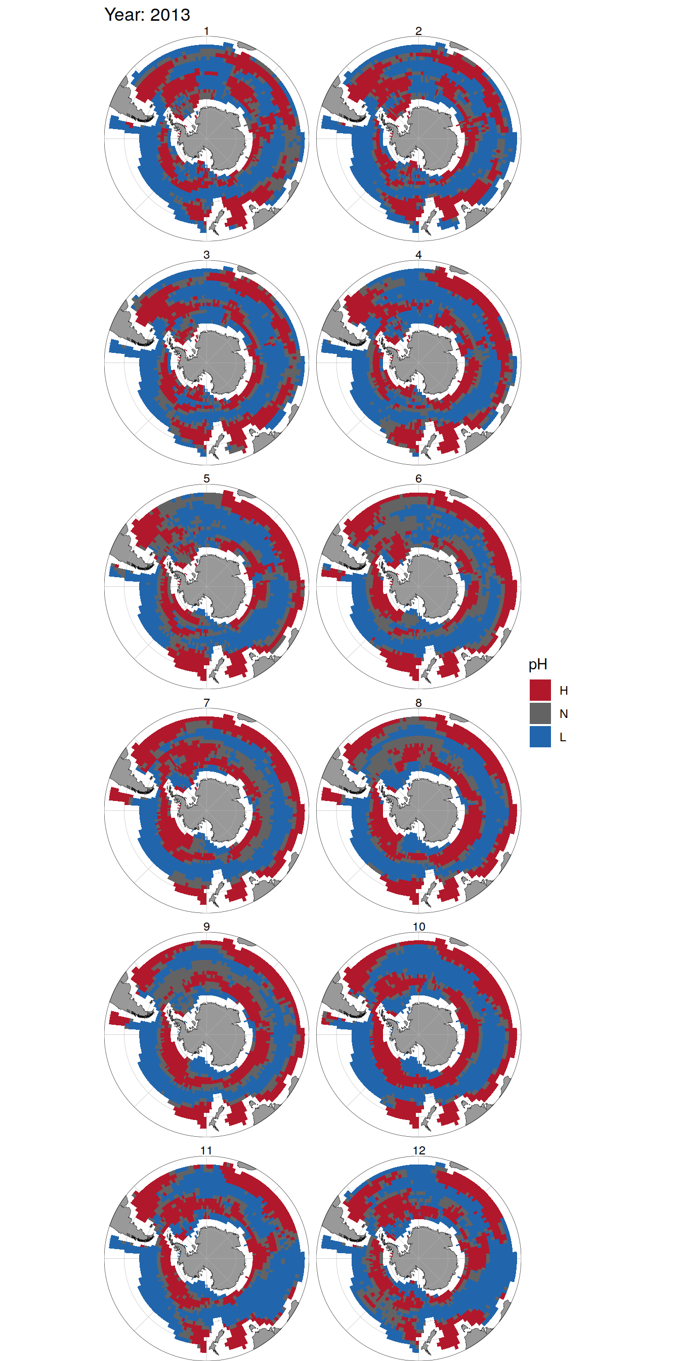
[[2]]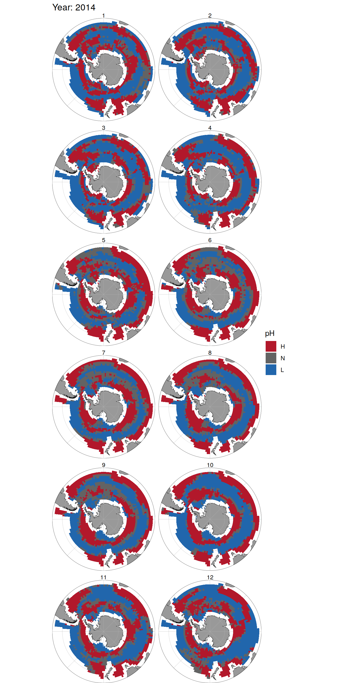
[[3]]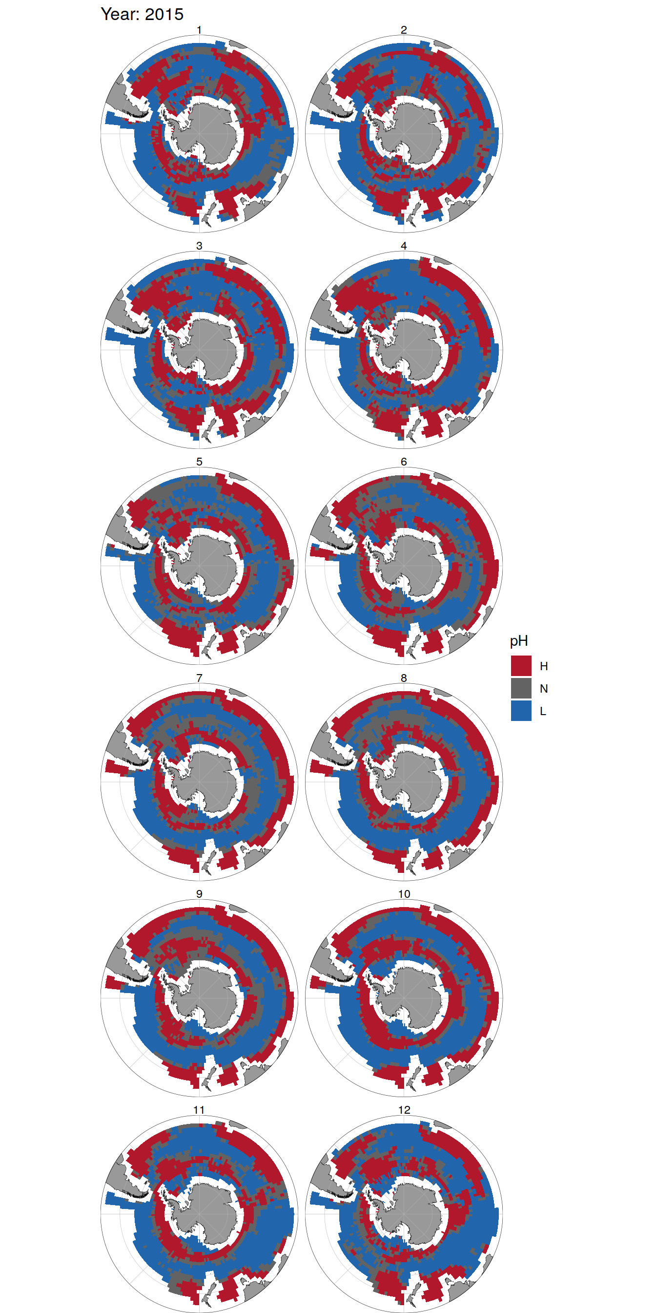
[[4]]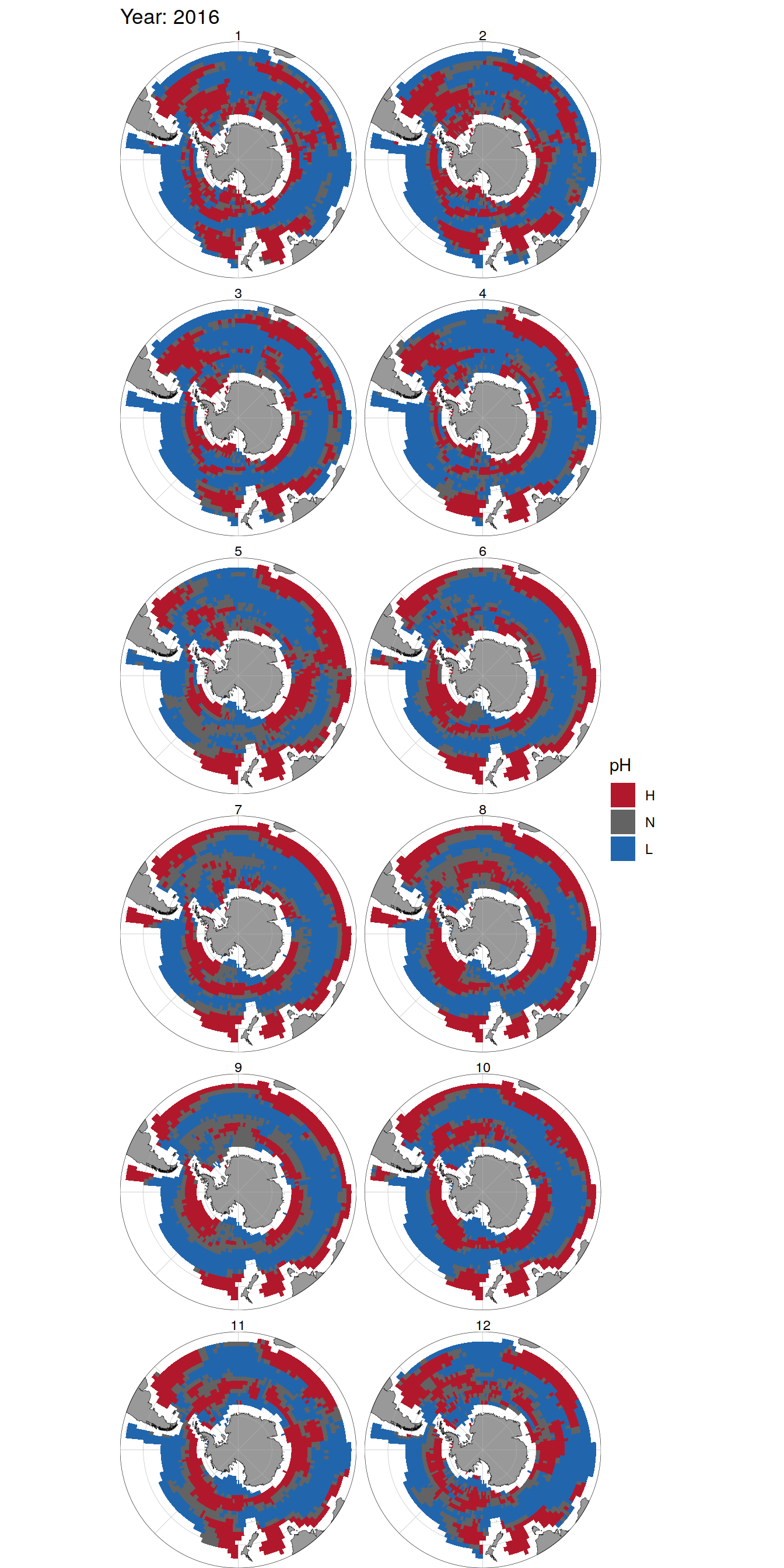
[[5]]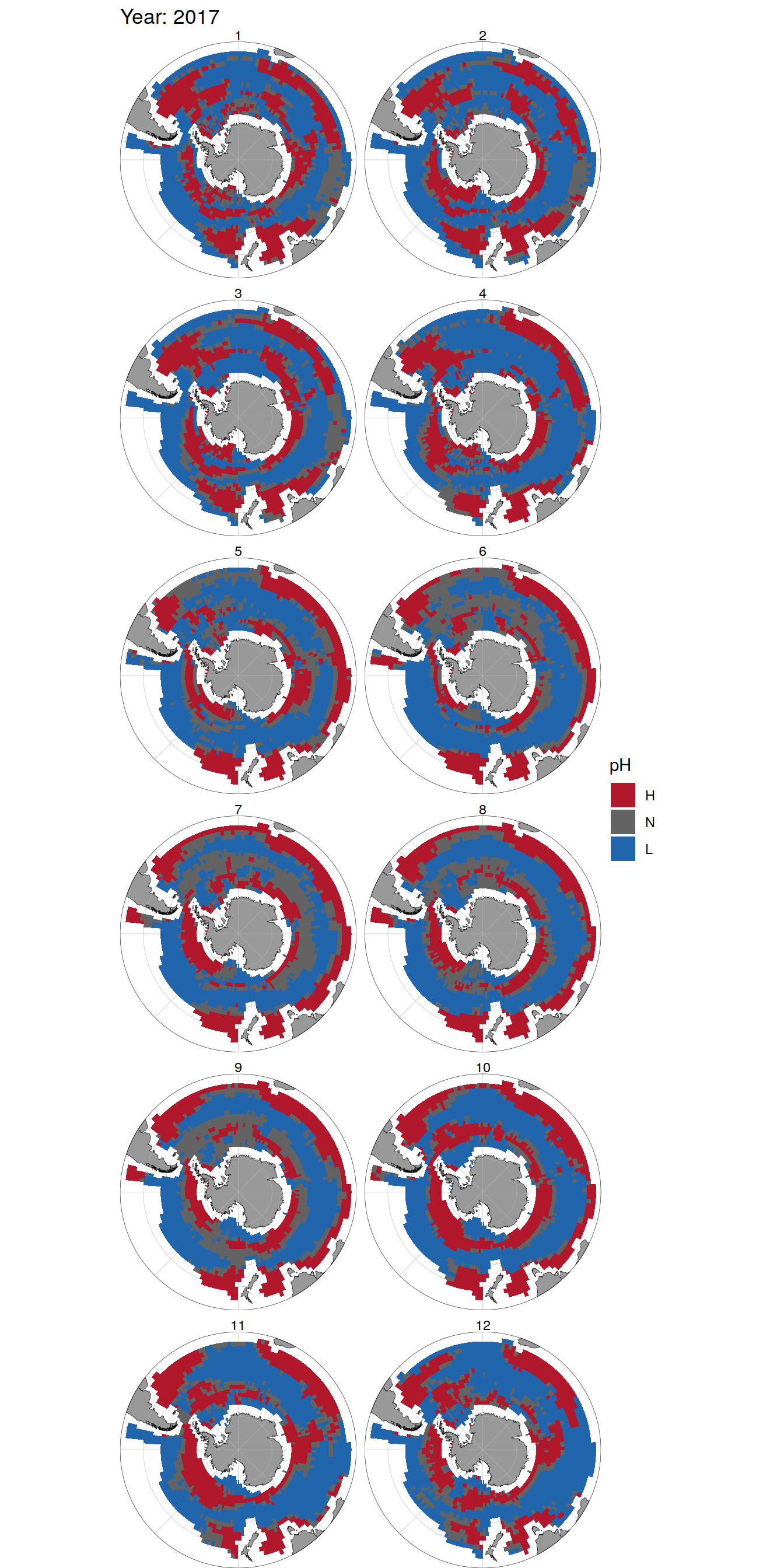
[[6]]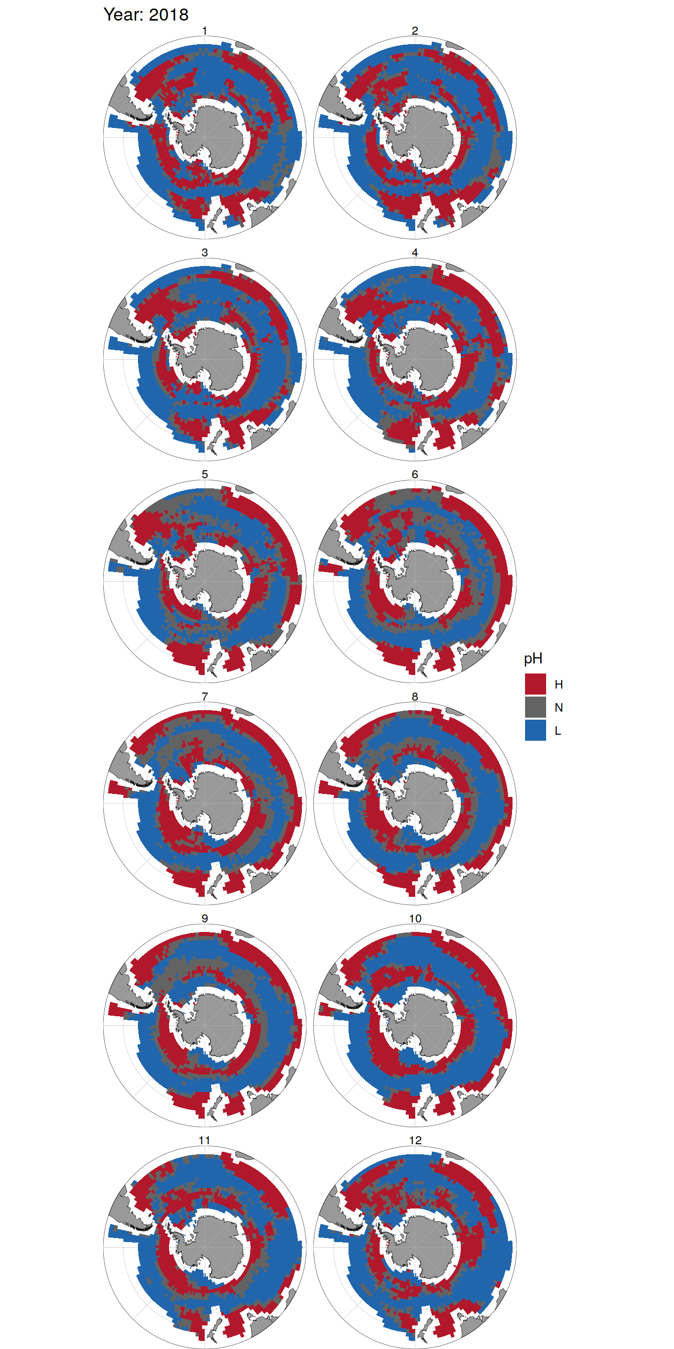
[[7]]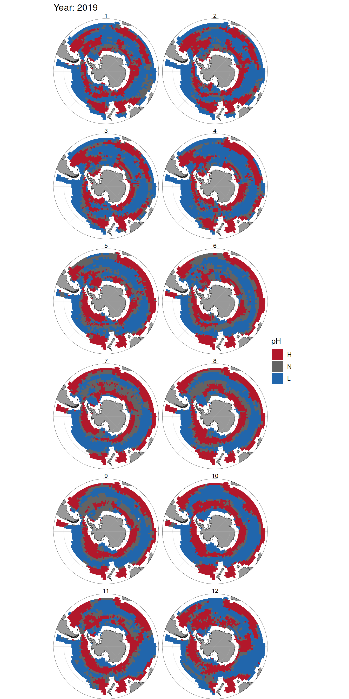
[[8]]
Anomaly time series
# calculate a regional mean pH for each biome, basin, and ph extreme (H/L/N) and plot a timeseries

OceanSODA_2x2_SO_extreme_biome %>%
  group_by(date, biome, basin_AIP, ph_extreme) %>%
  summarise(ph_regional = mean(ph_total, na.rm = TRUE)) %>%
  ungroup() %>%
  ggplot(aes(x = date, y = ph_regional, col = ph_extreme))+
  geom_point(size = 0.3)+
  geom_line()+
  scale_color_manual(values = HNL_colors) +
  facet_grid(basin_AIP~biome)+
  labs(x = 'date',
       y = 'regional mean pH',
       col = 'pH anomaly') +
  theme(legend.position = 'bottom')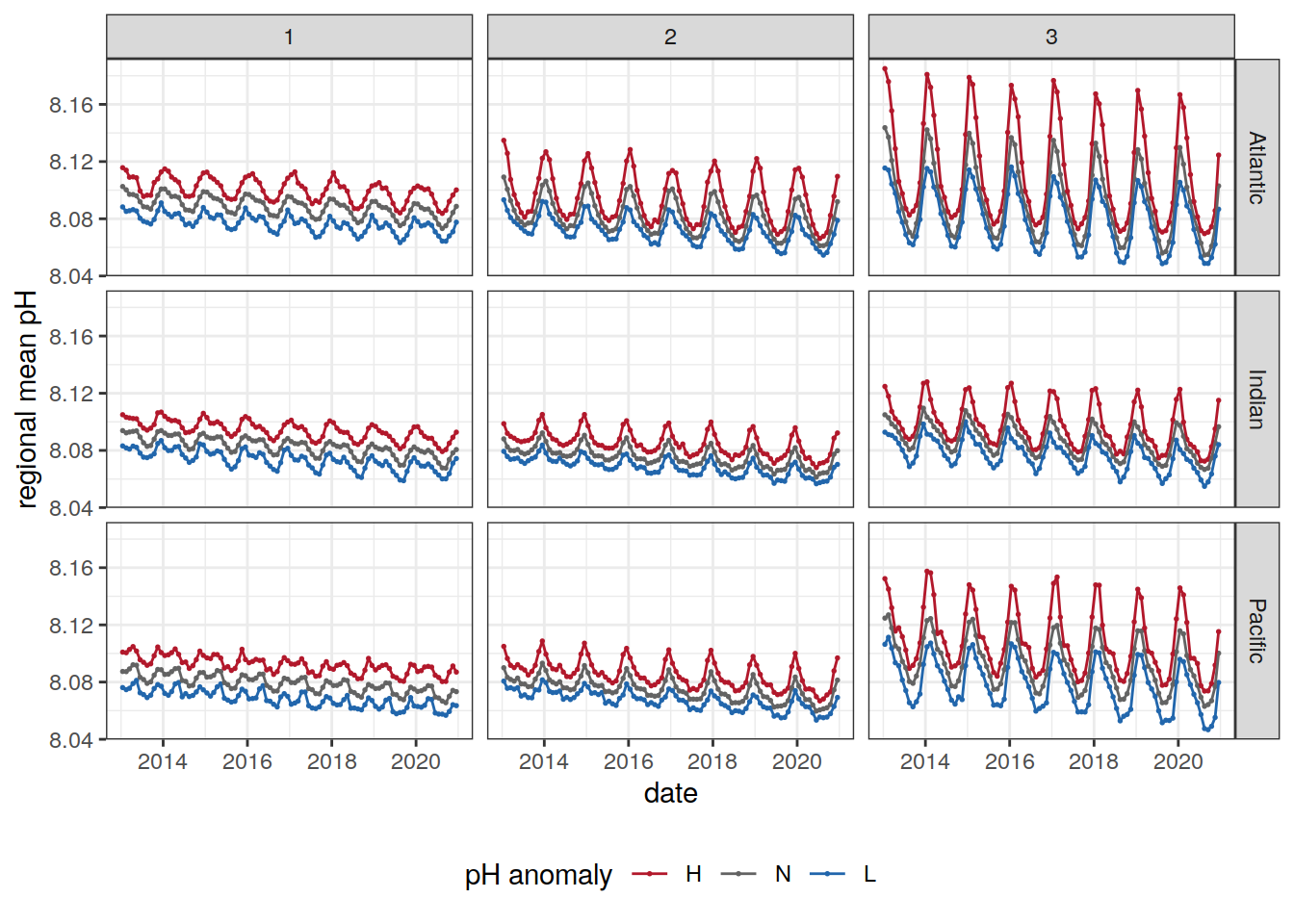
Anomaly histogram
OceanSODA_2x2_SO_extreme_biome %>%
  ggplot(aes(ph_total, col = ph_extreme)) +
  geom_density() +
  scale_color_manual(values = HNL_colors) +
  facet_grid(basin_AIP ~ biome) +
  coord_cartesian(xlim = c(8, 8.2)) +
  labs(x = 'value',
       y = 'density',
       col = 'pH anomaly') +
  theme(legend.position = 'bottom')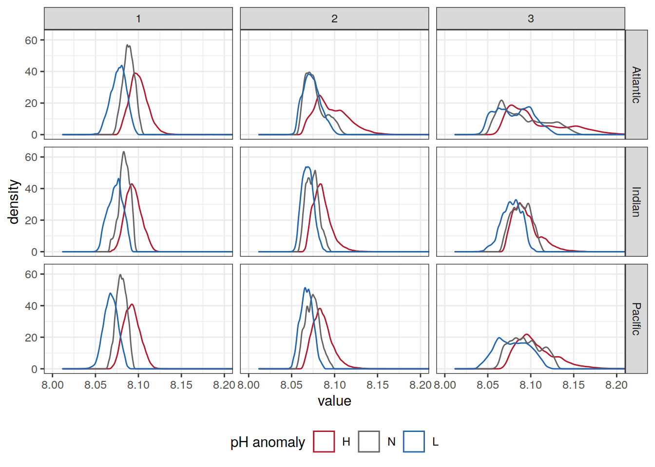
Threshold histogram
OceanSODA_2x2_SO_extreme_biome %>%
  mutate(ph_extreme = as.double(ph_extreme)) %>%
  pivot_longer(starts_with("ph_"),
               names_to = "level",
               values_to = "value",
               names_prefix = "ph_") %>%
  ggplot(aes(value, col = level)) +
  geom_density() +
  scale_color_manual(values = HNL_colors, name = "threshold") +
  coord_cartesian(xlim = c(8, 8.2)) +
  lims(y = c(0, 400))+
  theme(legend.position = 'bottom')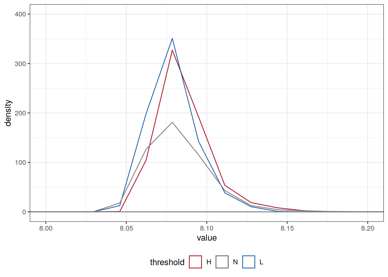
Argo
Join OceanSODA
# rename OceanSODA columns
OceanSODA_2x2_SO_extreme <- OceanSODA_2x2_SO_extreme_grid %>%
  rename(OceanSODA_ph = ph_total,
         OceanSODA_ph_uncert = ph_total_uncert)

# combine the argo profile data to the surface extreme data
profile_extreme <- inner_join(full_argo_2x2_SO, OceanSODA_2x2_SO_extreme)
Plot profiles
Argo profiles plotted according to the surface OceanSODA pH
L profiles correspond to a surface acidification event (low pH), as recorded in OceanSODA
H profiles correspond to an event of high surface pH, as recorded in OceanSODA
N profiles correspond to normal surface OceanSODA pH
pH
profile_extreme %>%
  group_split(biome, basin_AIP, year) %>%
  # head(5) %>%
  map(
    ~ ggplot(
      data = .x,
      aes(
        x = ph_in_situ_total_adjusted,
        y = depth,
        group = ph_extreme,
        col = ph_extreme
      )
    ) +
      geom_point(pch = 19, size = 0.3) +
      scale_y_reverse() +
      scale_color_manual(values = HNL_colors) +
      facet_wrap(~ month, ncol = 6) +
      labs(
        x = 'Argo pH (total scale)',
        y = 'depth (m)',
        title = paste(
          unique(.x$basin_AIP),
          "|",
          unique(.x$year),
          "| biome:",
          unique(.x$biome)
        ),
        col = 'OceanSODA pH \nanomaly'
      )
  )
[[1]]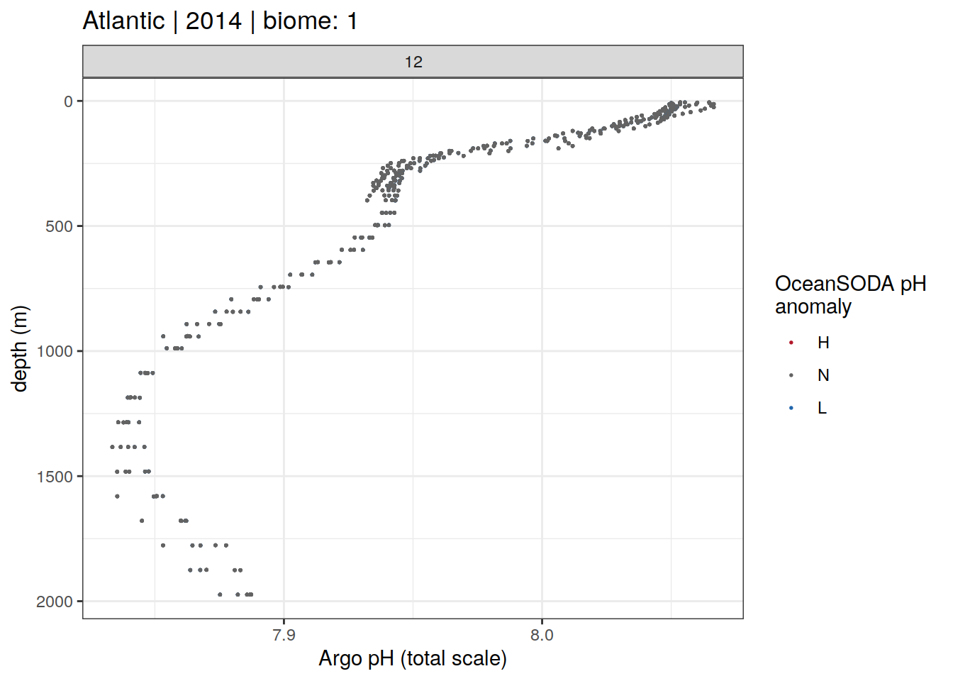
[[2]]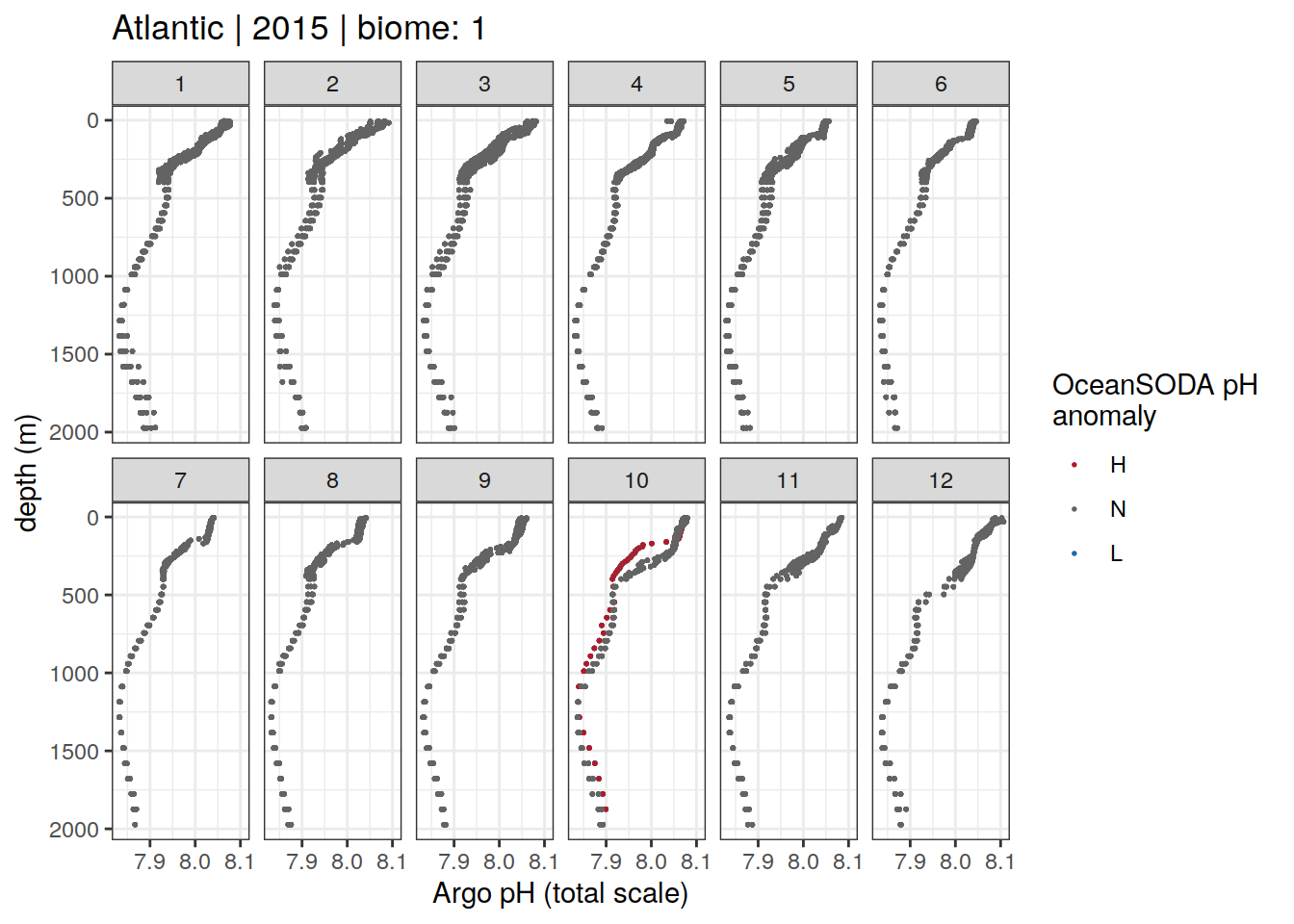
[[3]]
[[4]]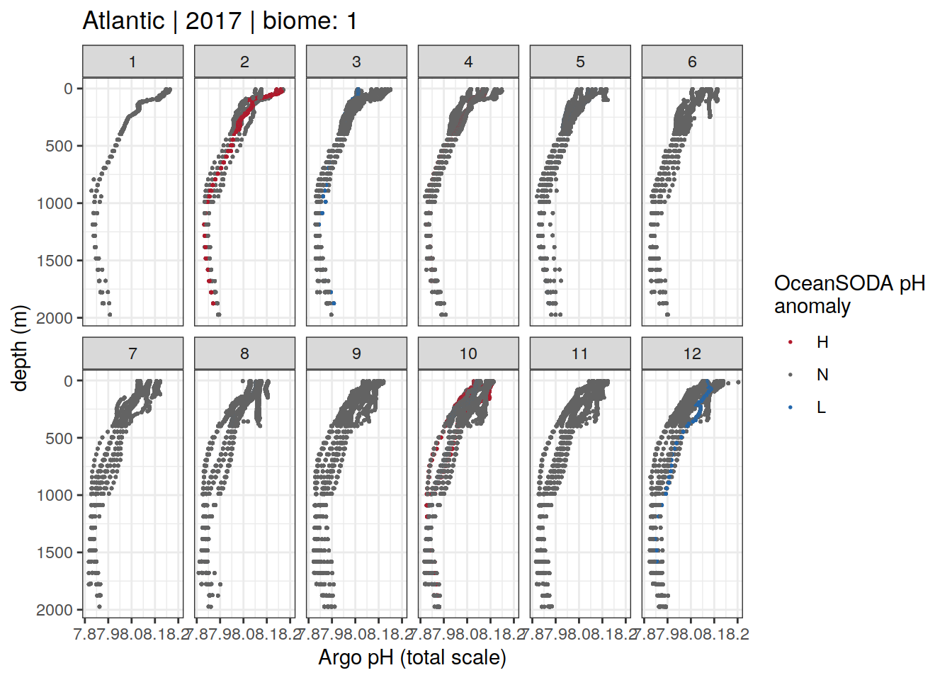
[[5]]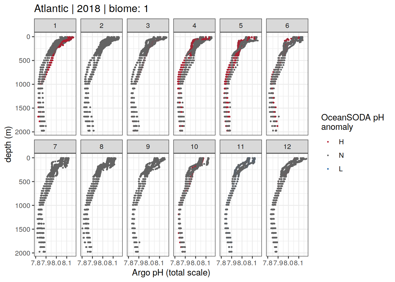
[[6]]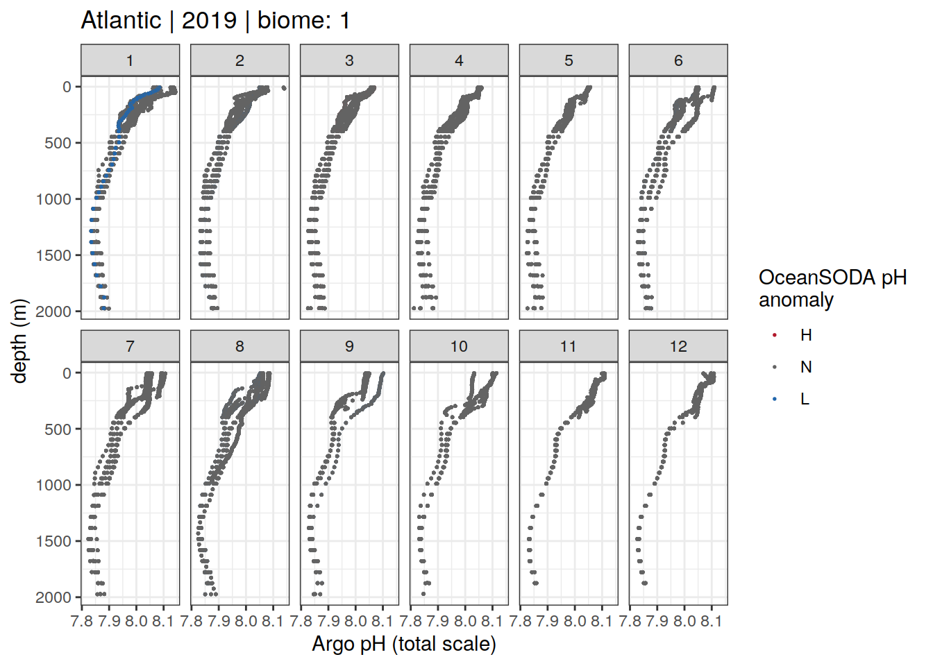
[[7]]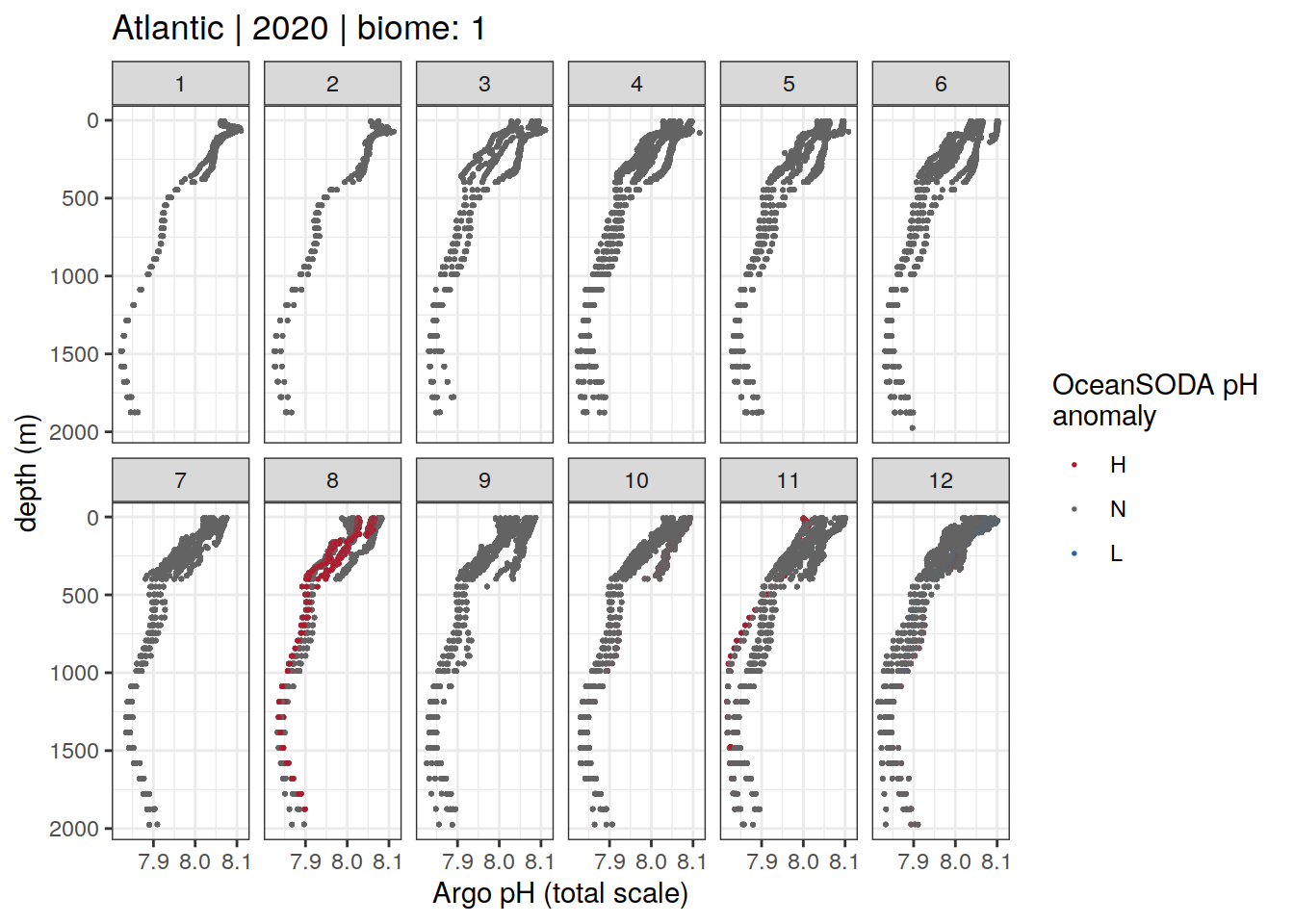
[[8]]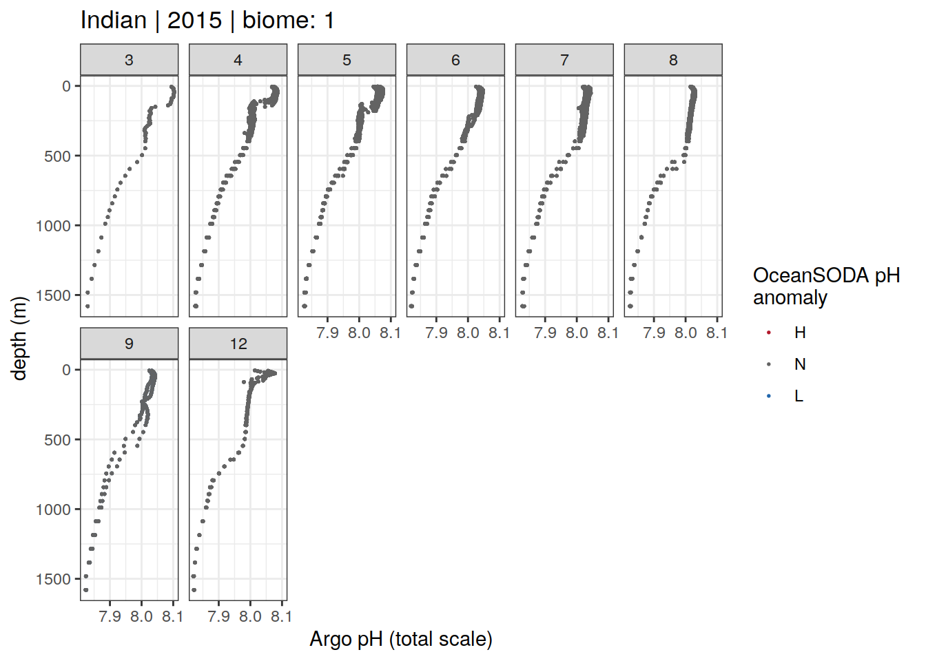
[[9]]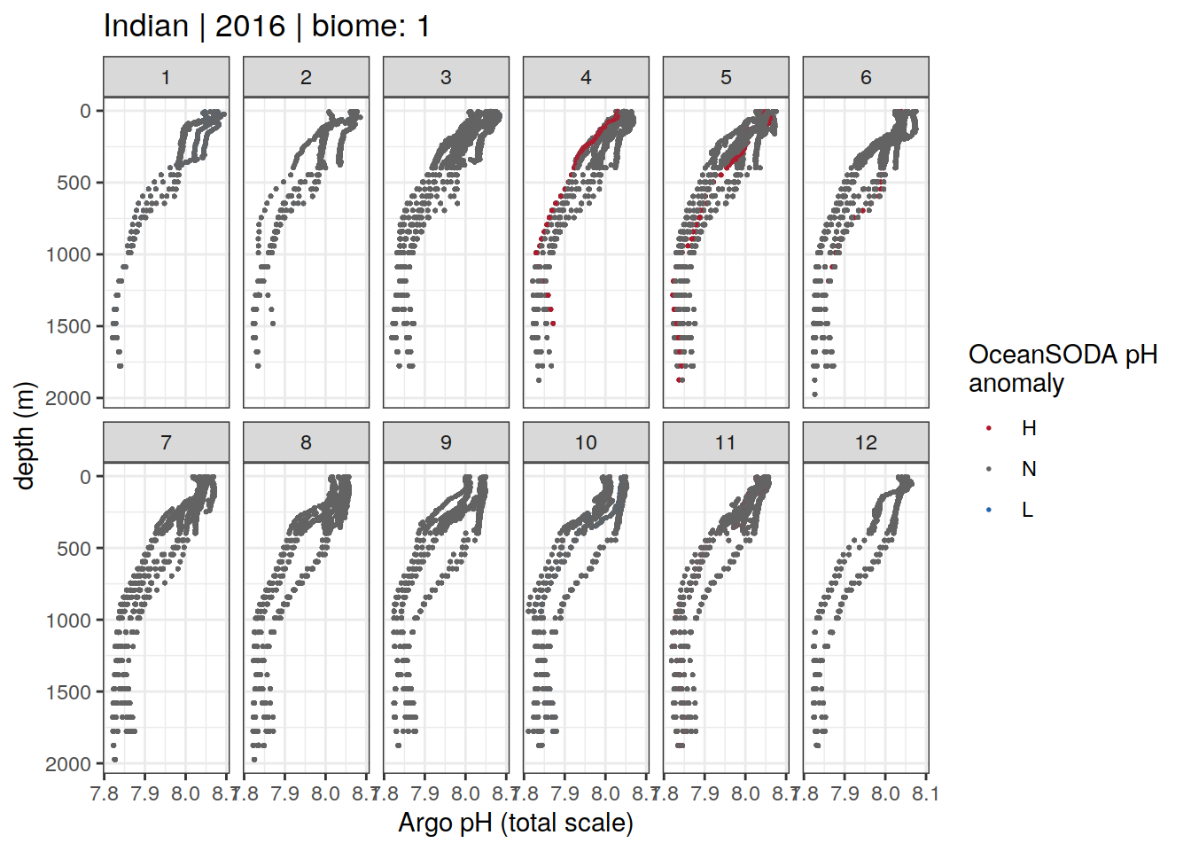
[[10]]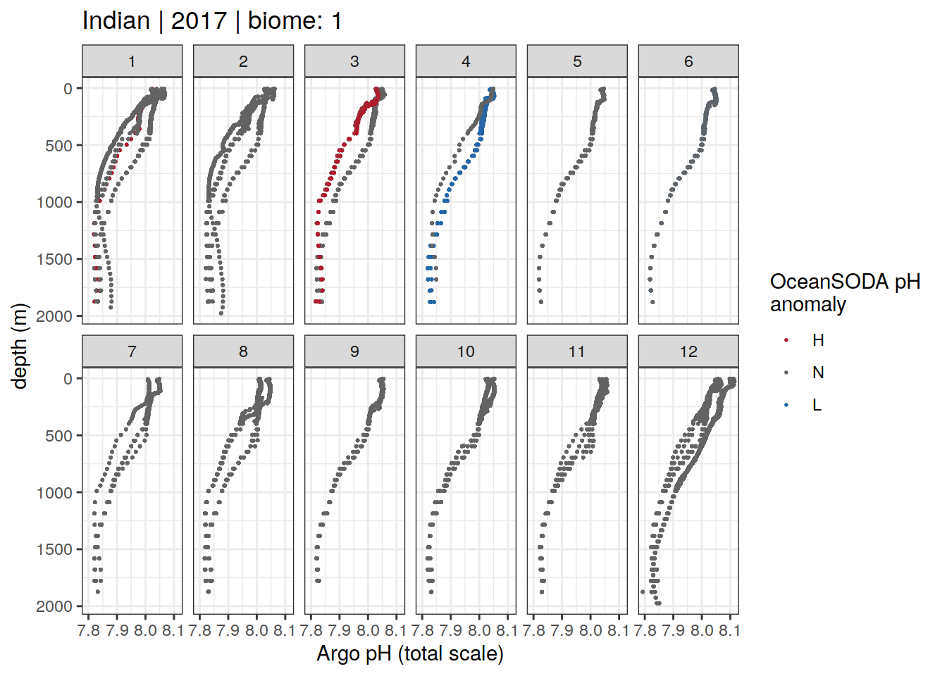
[[11]]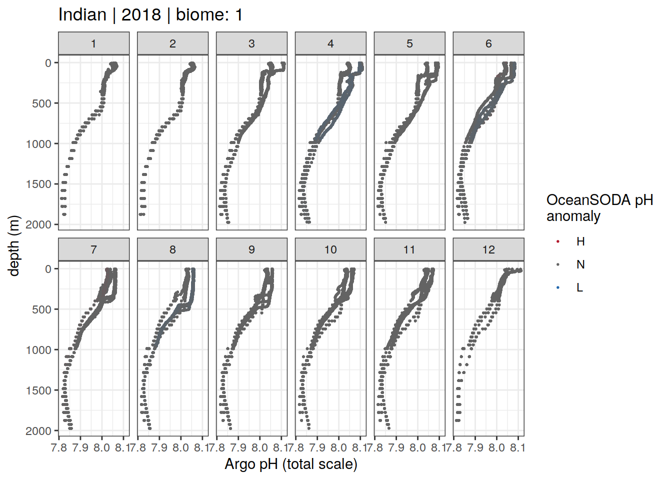
[[12]]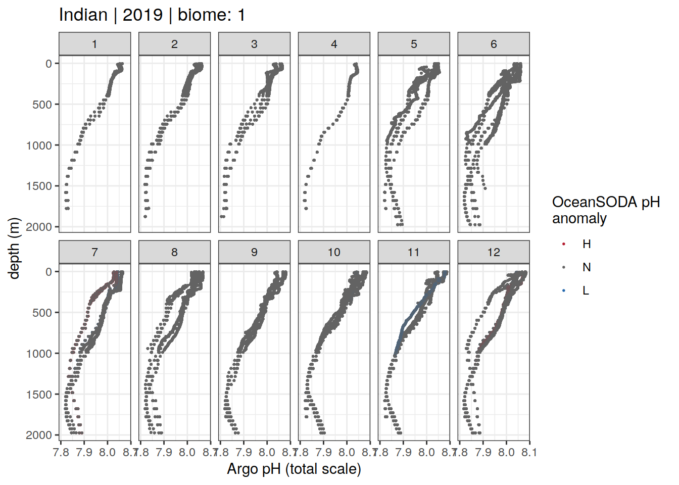
[[13]]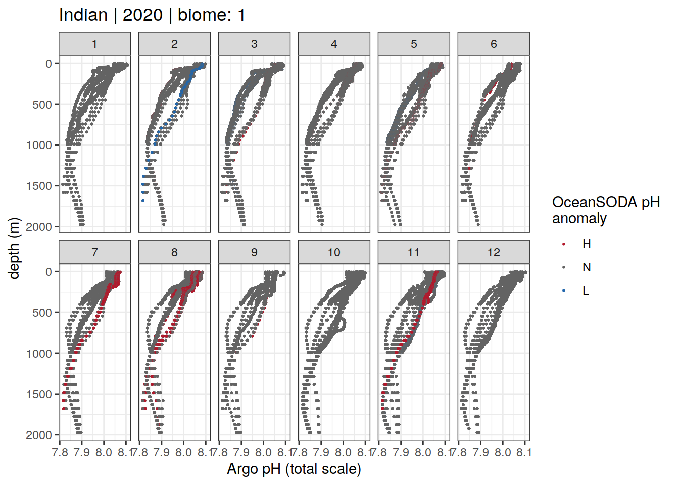
[[14]]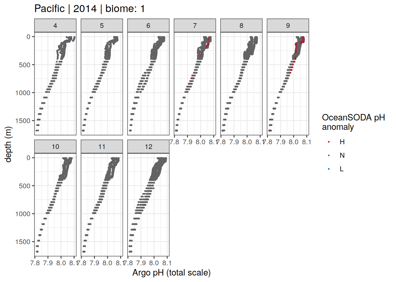
[[15]]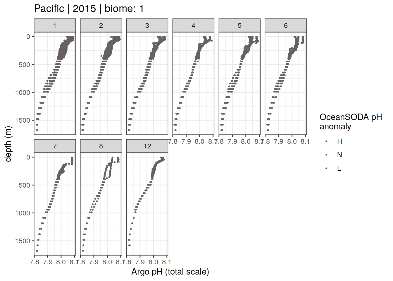
[[16]]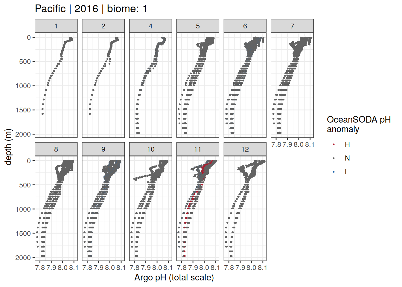
[[17]]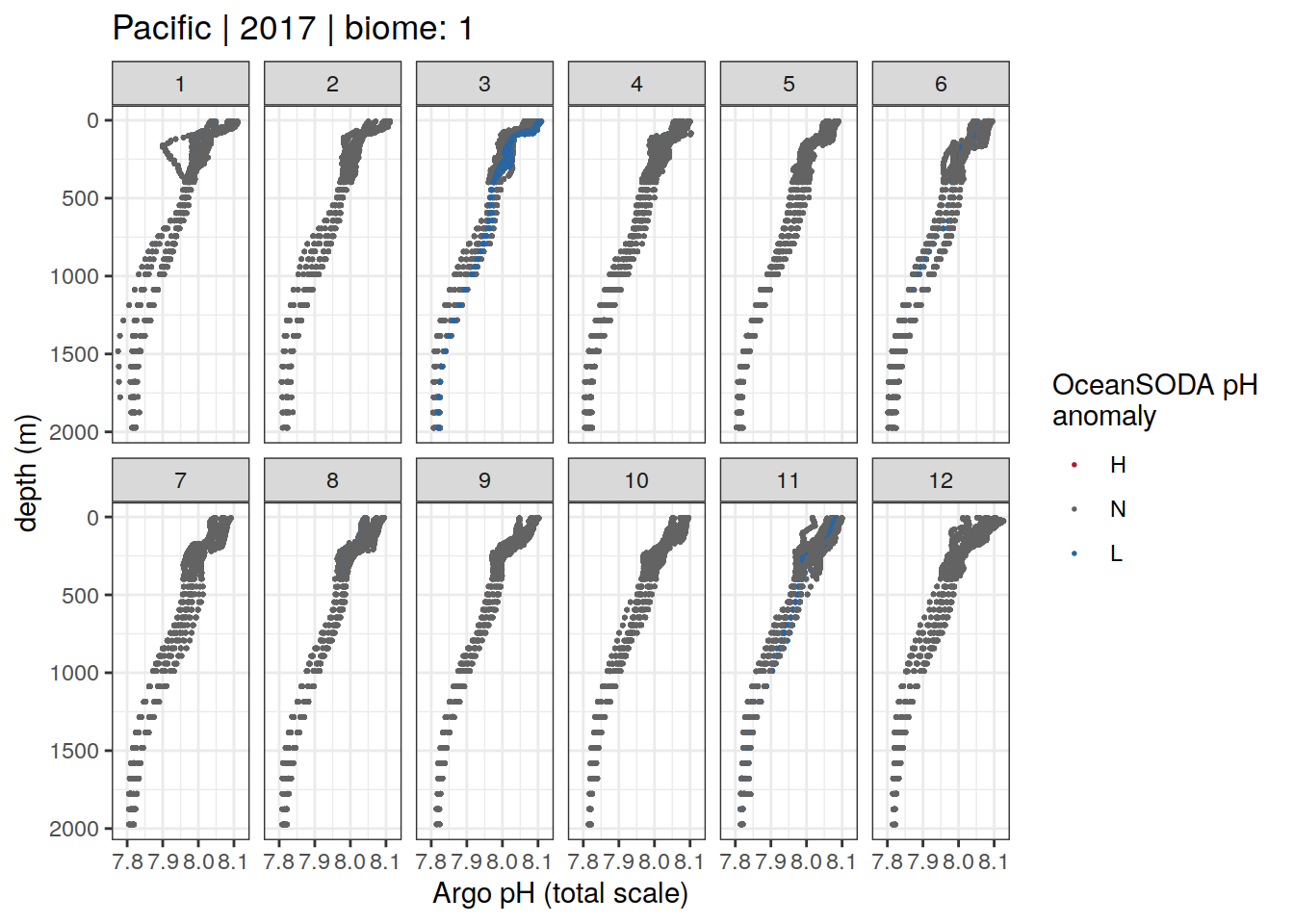
[[18]]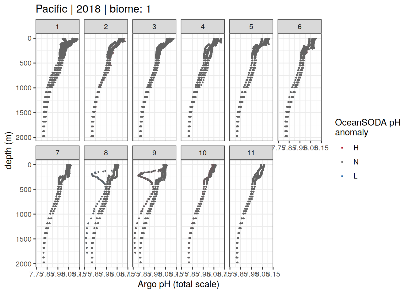
[[19]]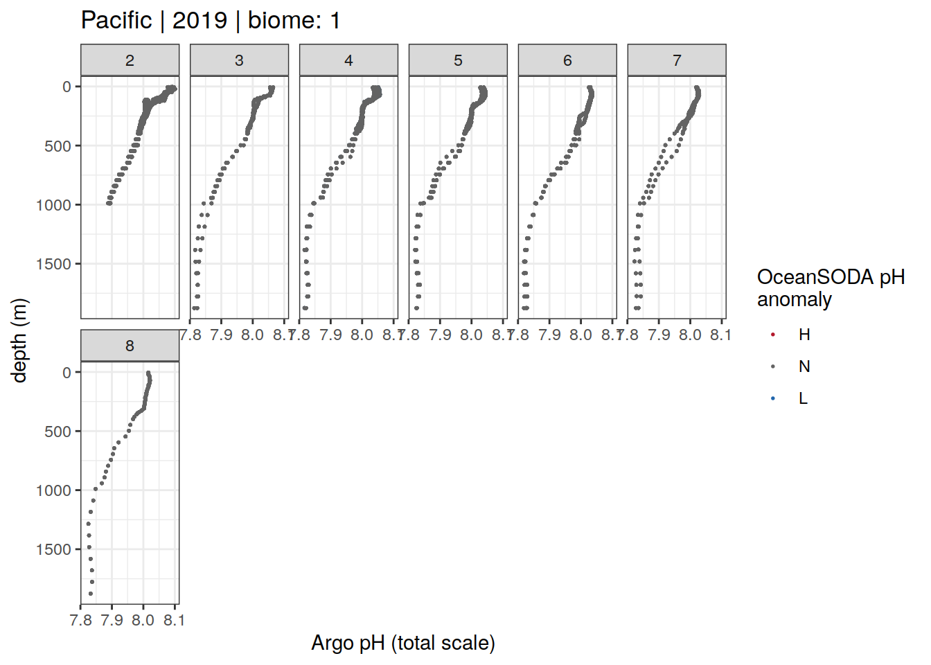
[[20]]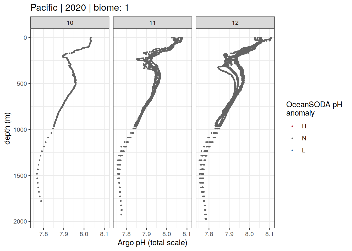
[[21]]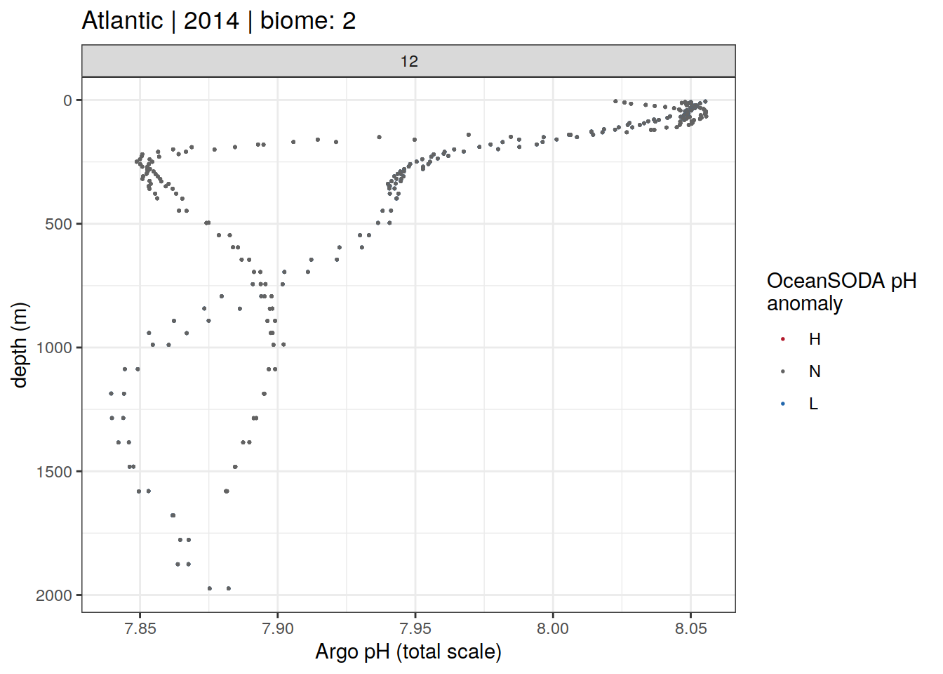
[[22]]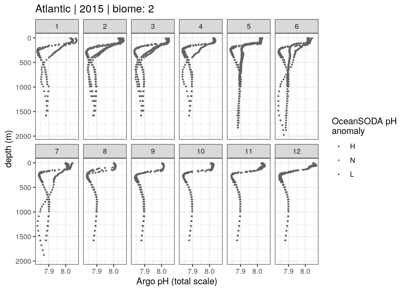
[[23]]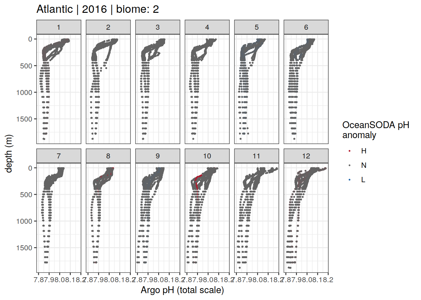
[[24]]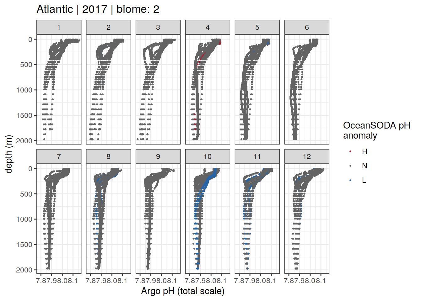
[[25]]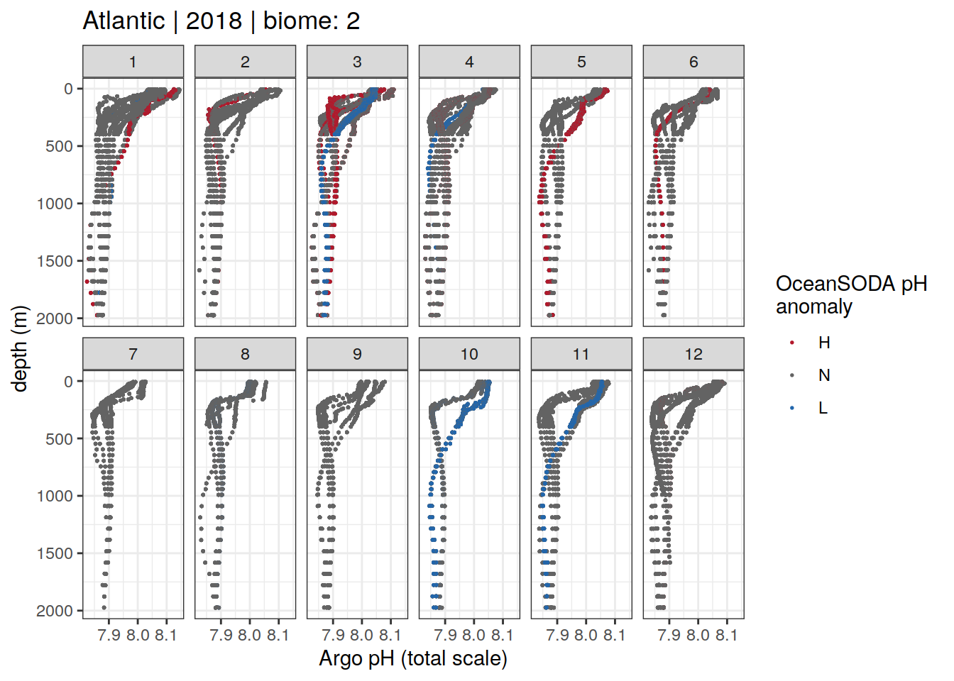
[[26]]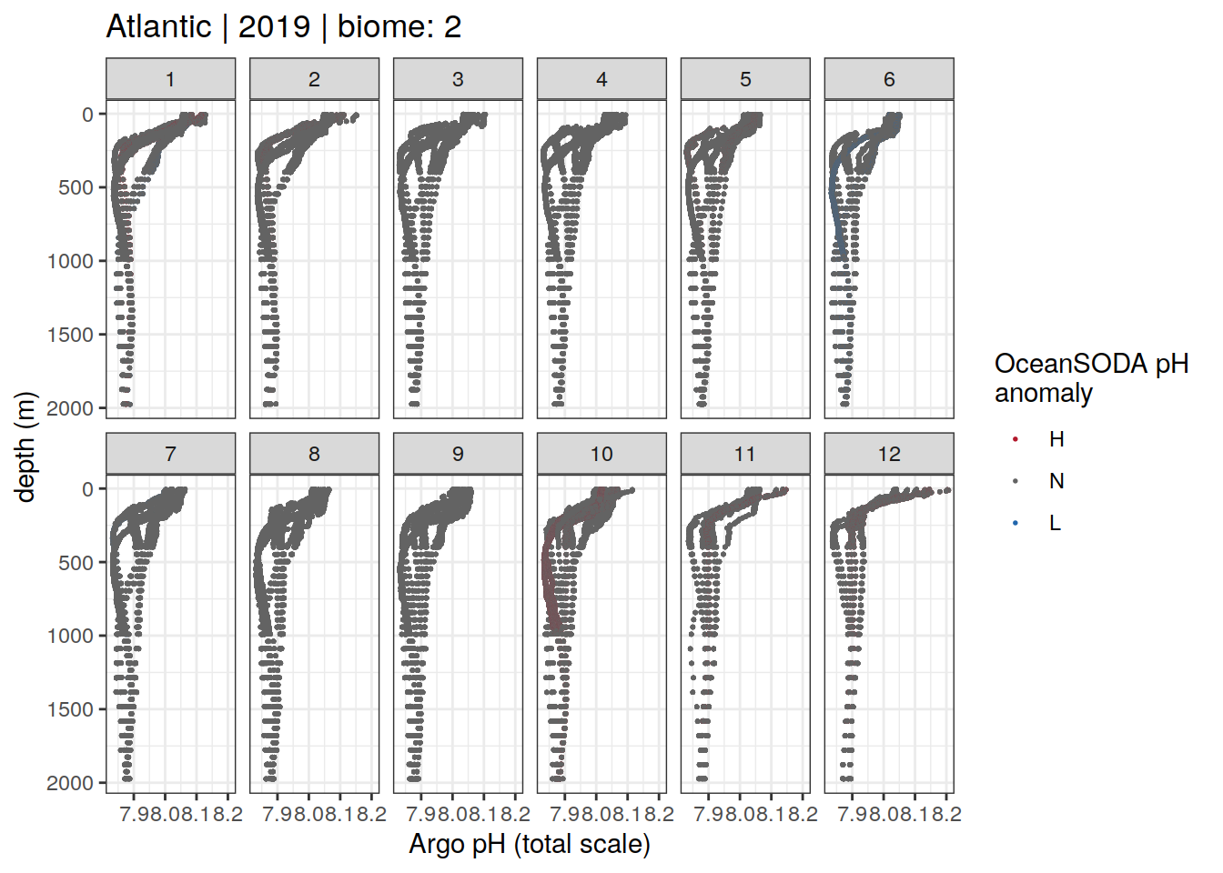
[[27]]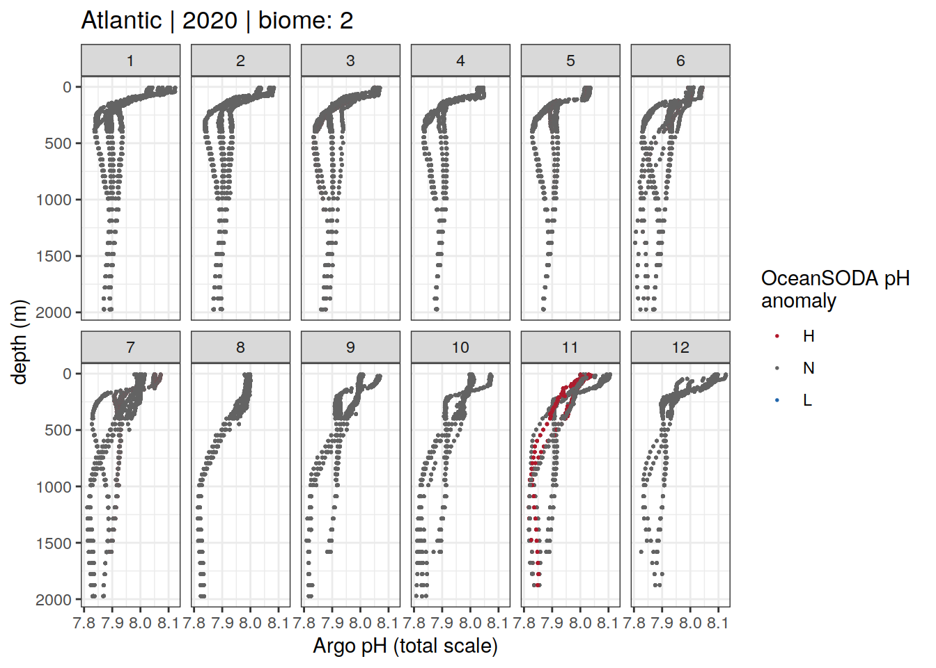
[[28]]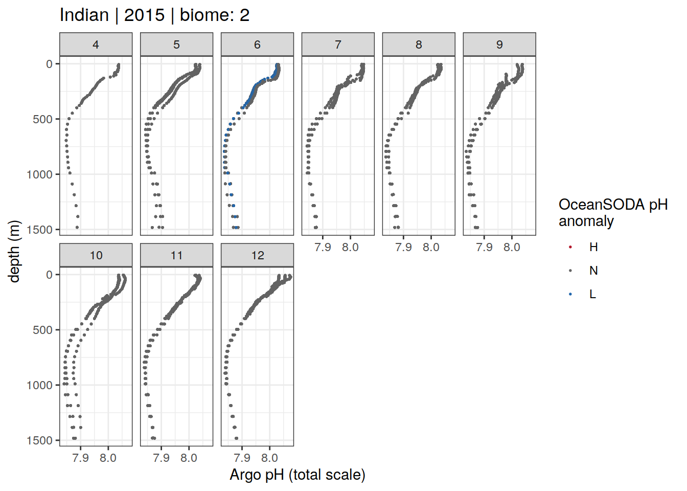
[[29]]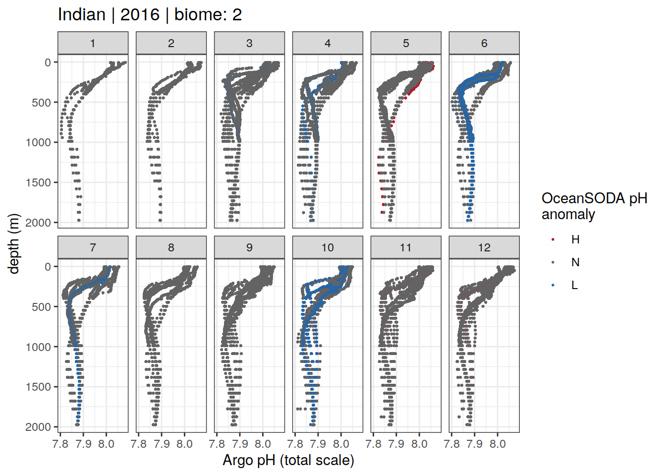
[[30]]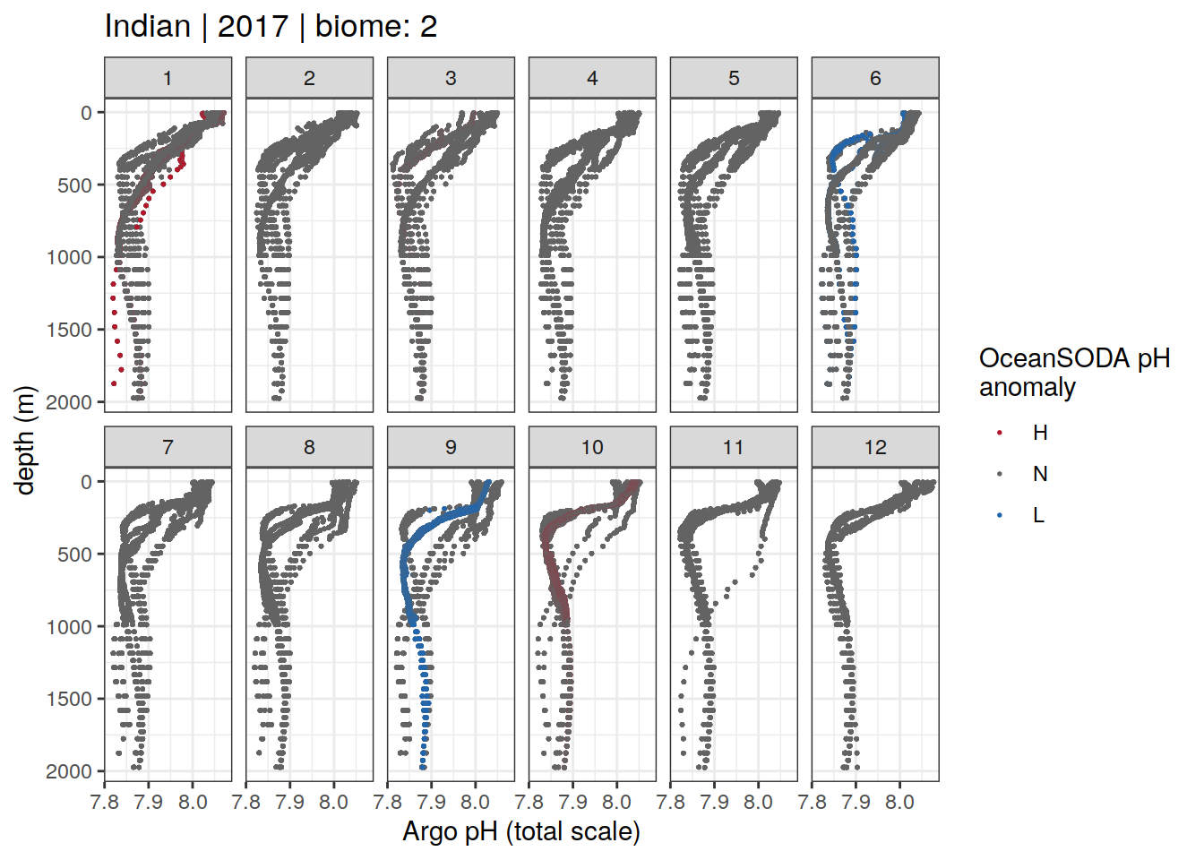
[[31]]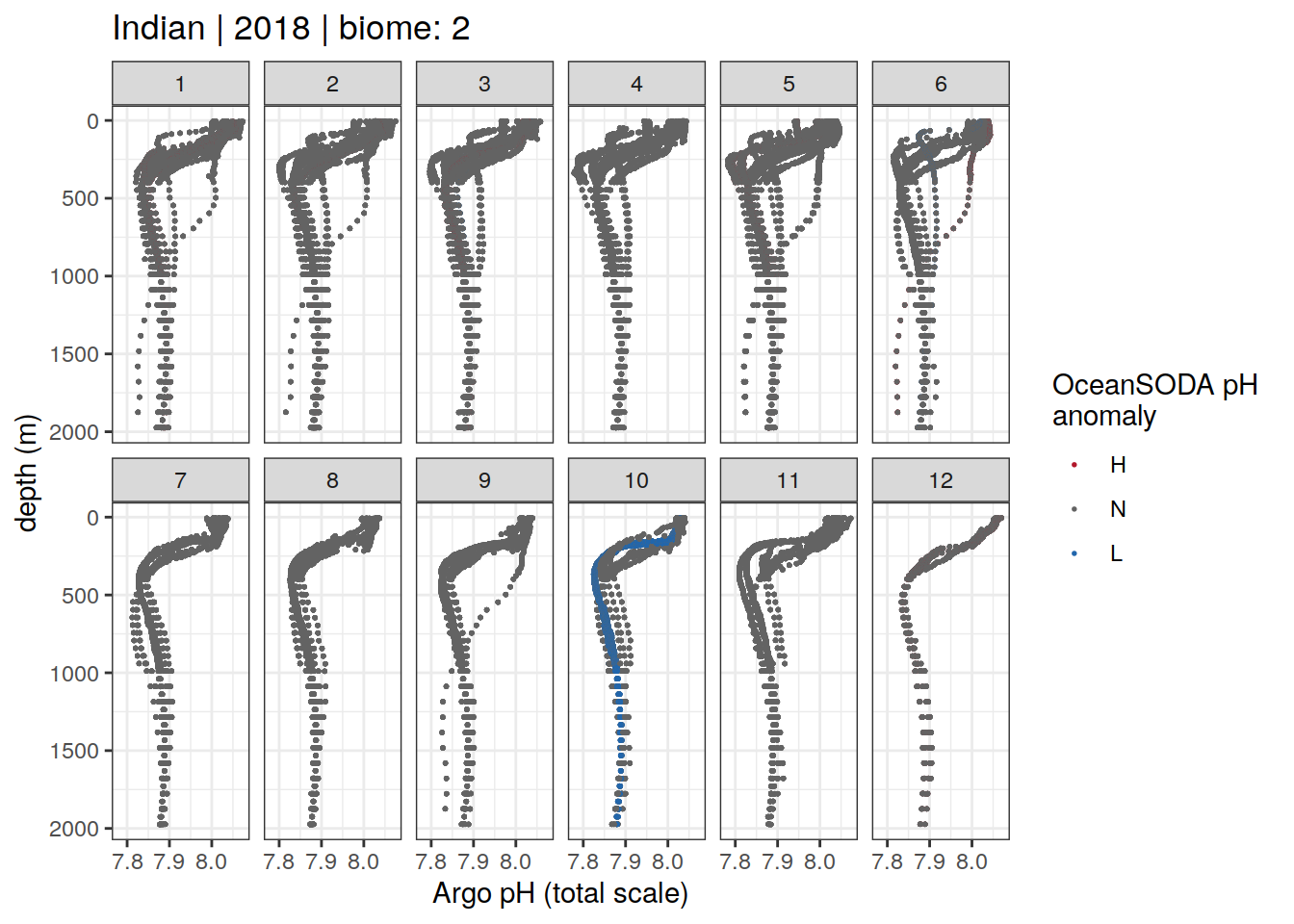
[[32]]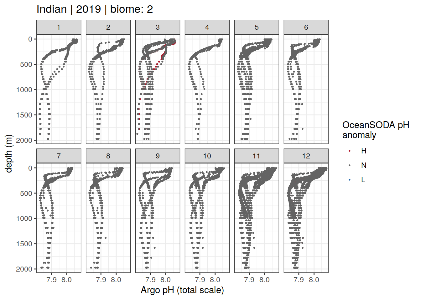
[[33]]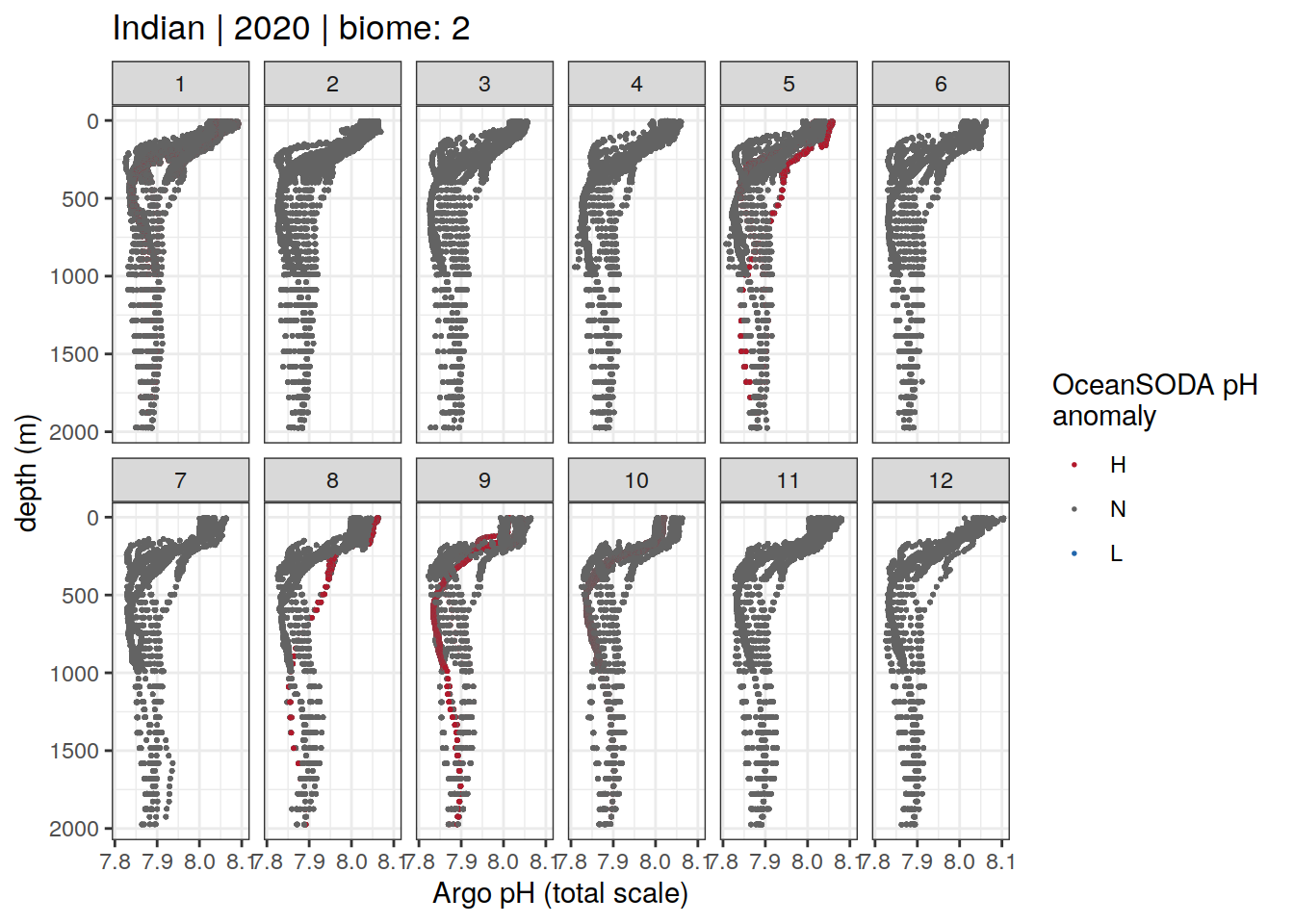
[[34]]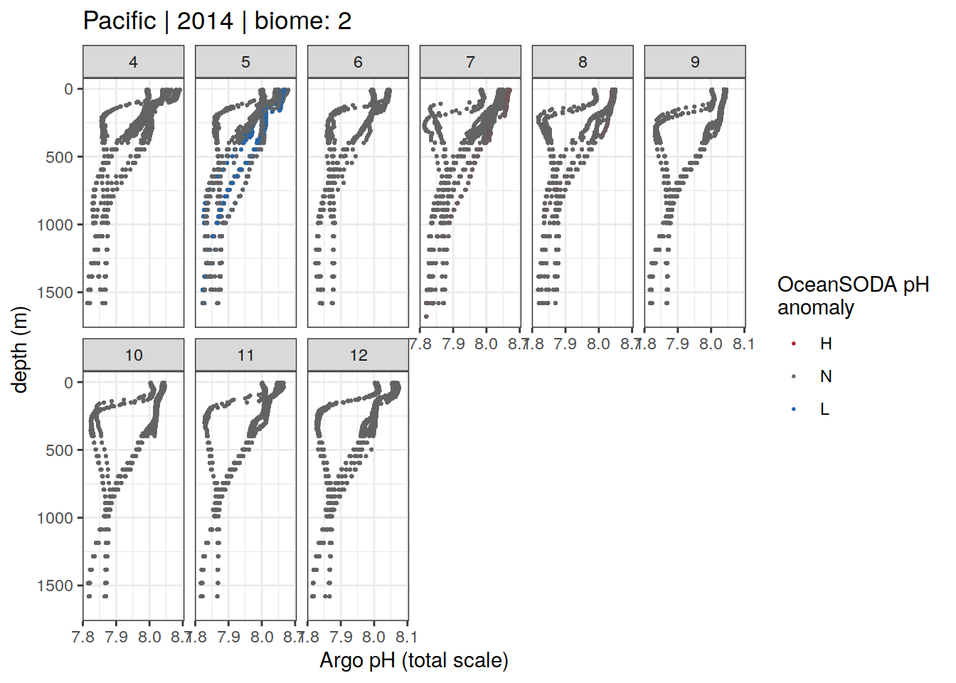
[[35]]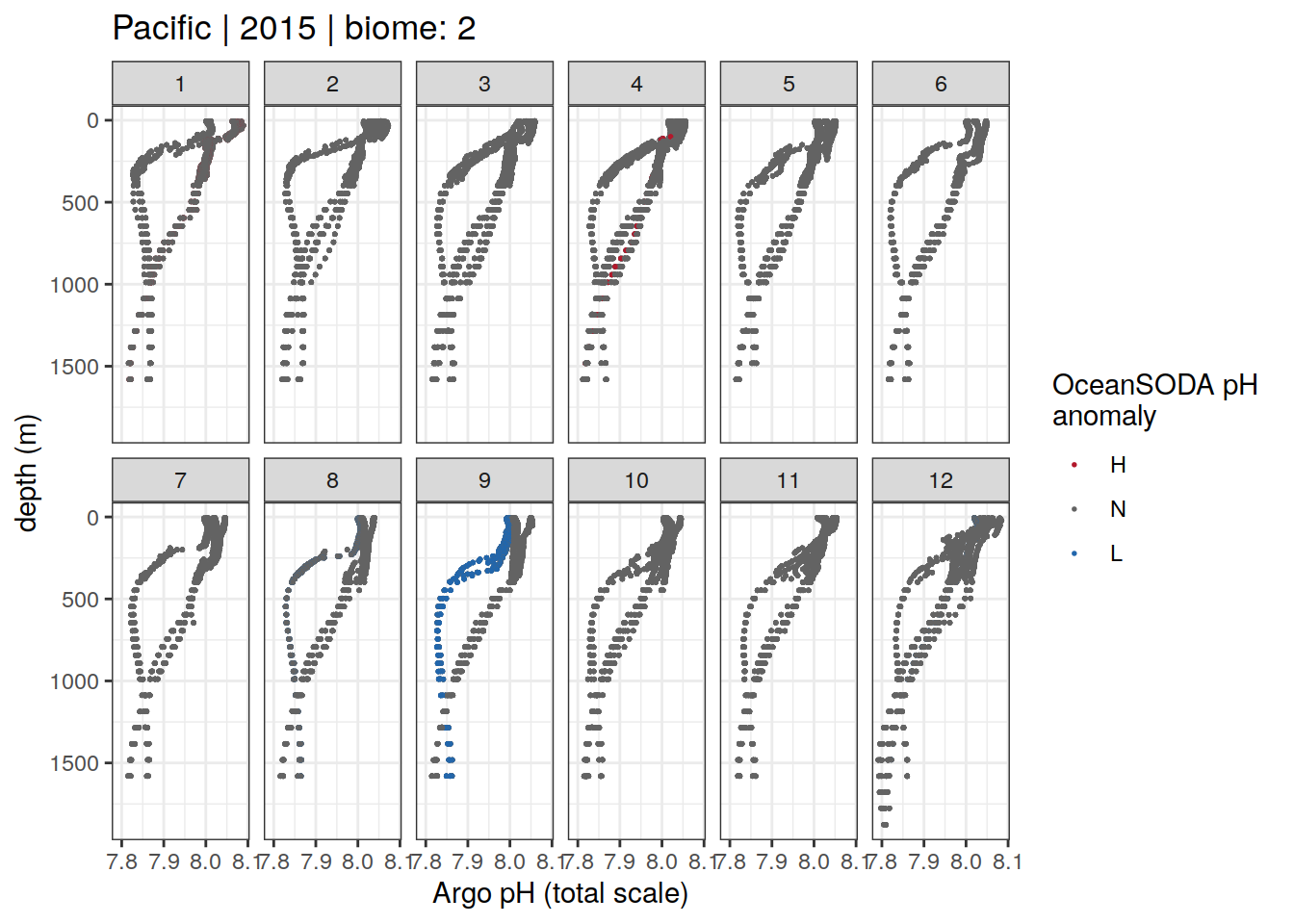
[[36]]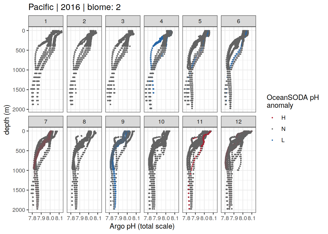
[[37]]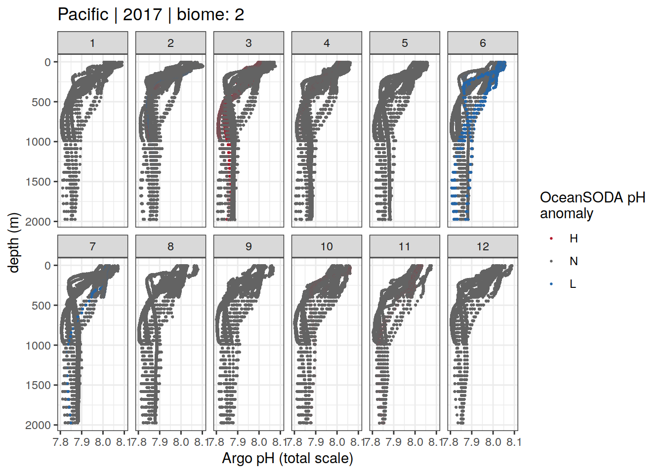
[[38]]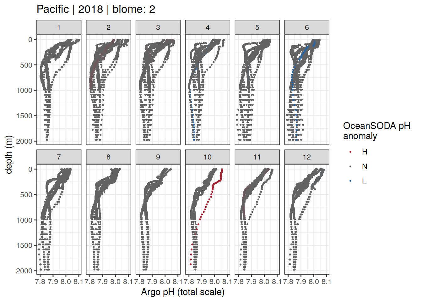
[[39]]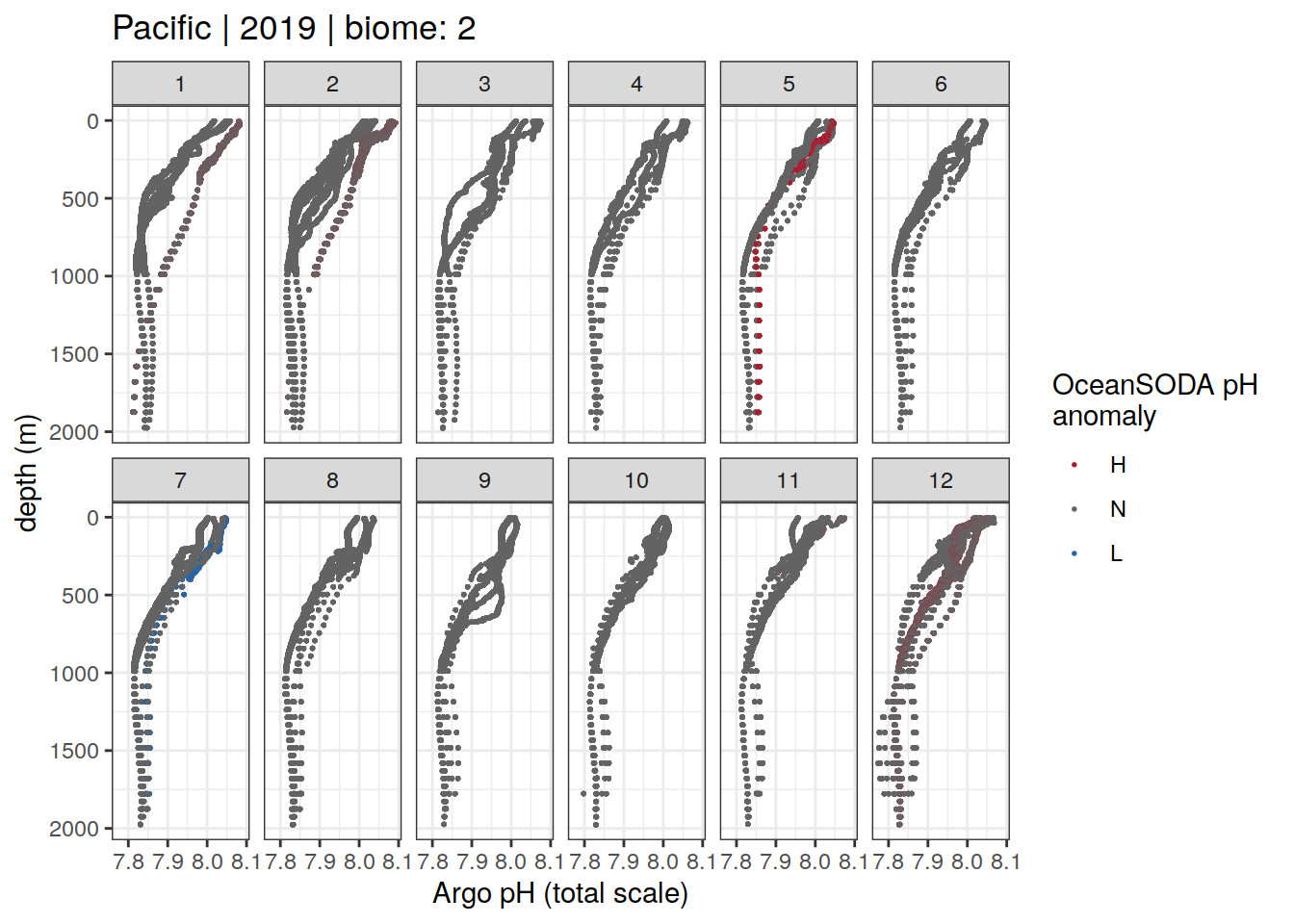
[[40]]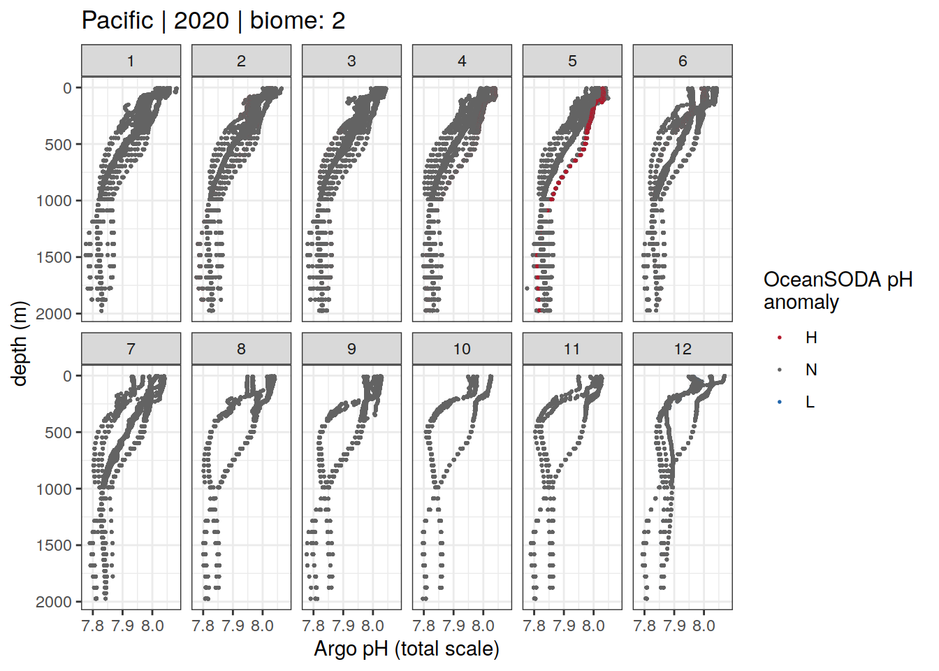
[[41]]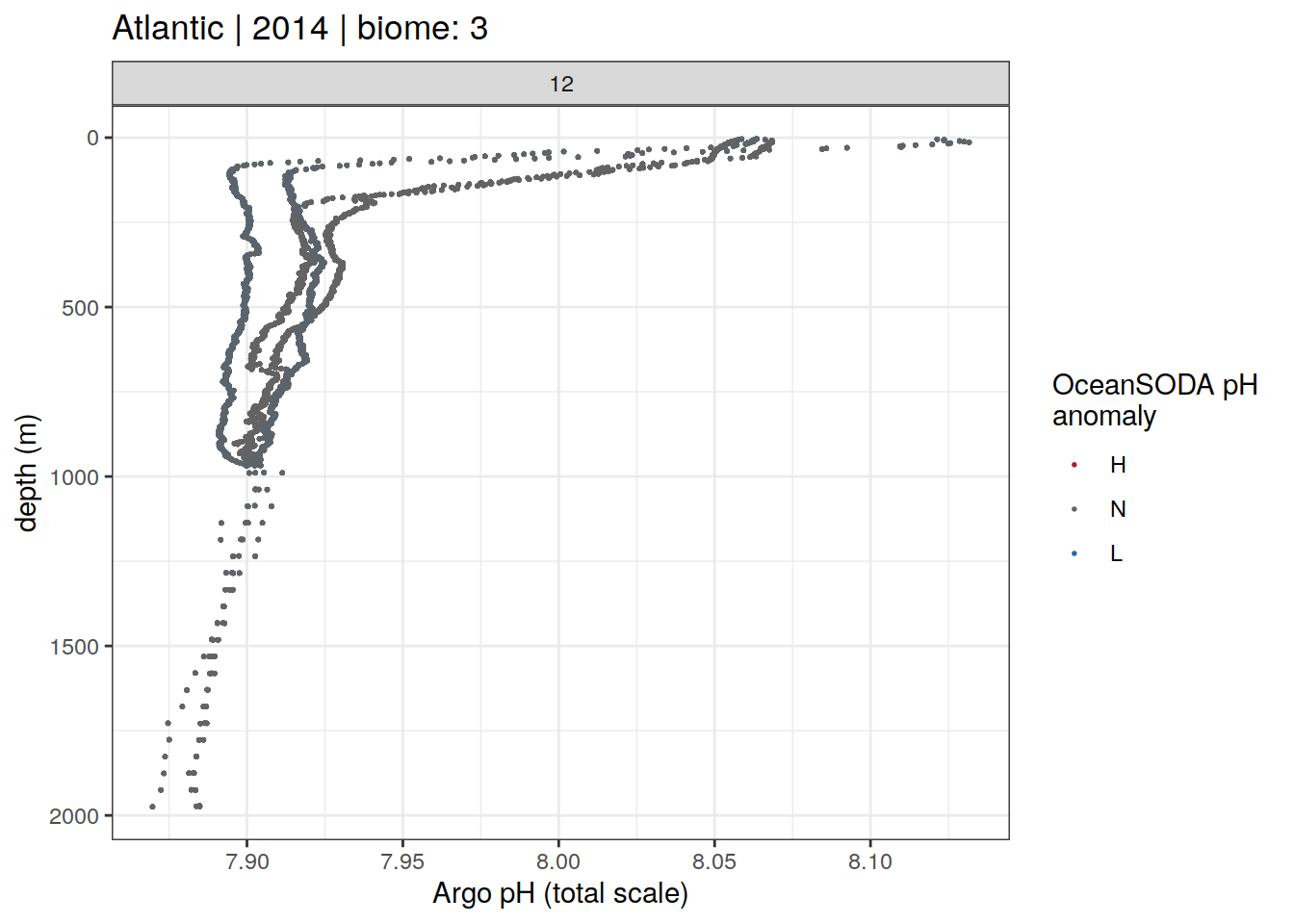
[[42]]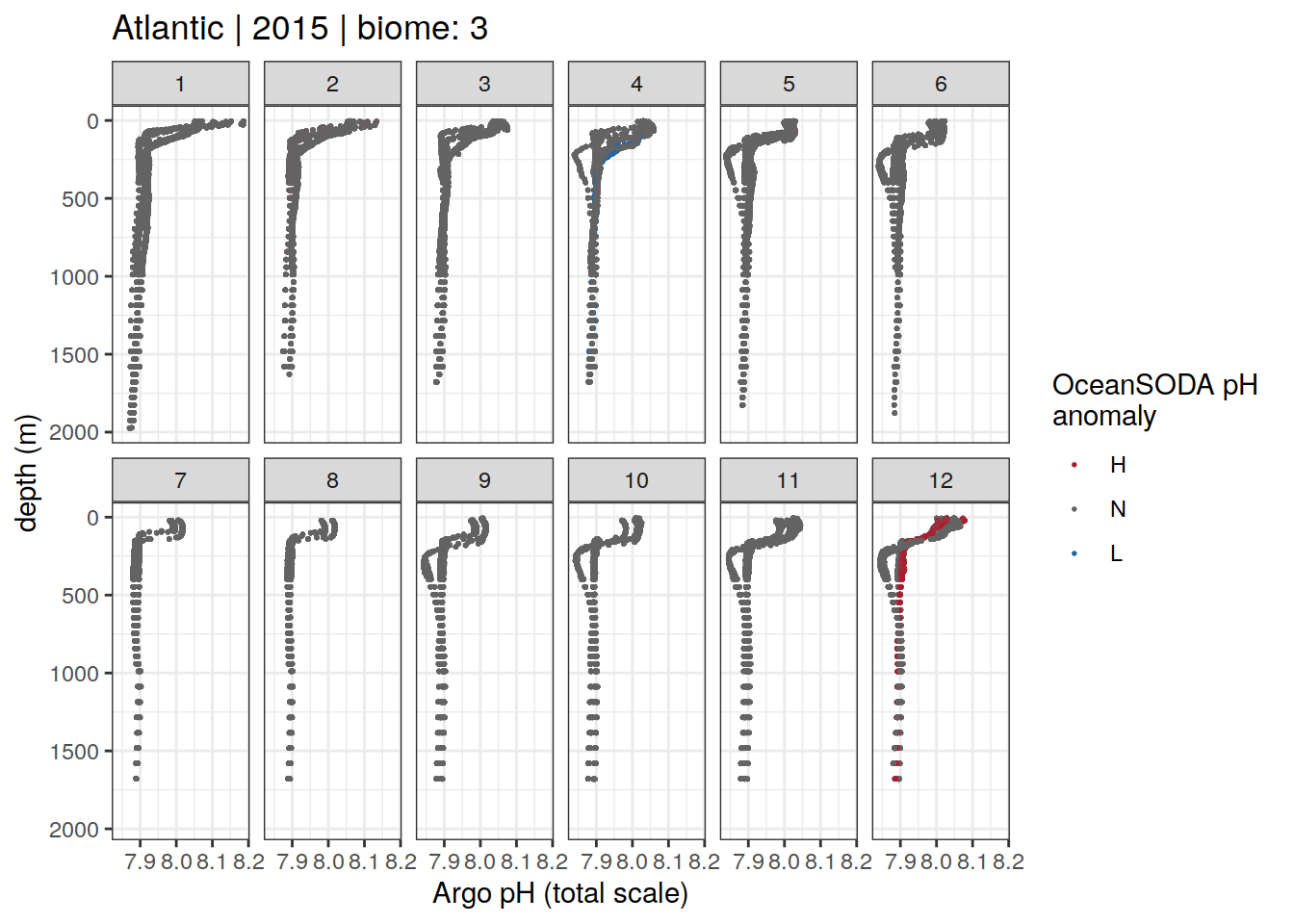
[[43]]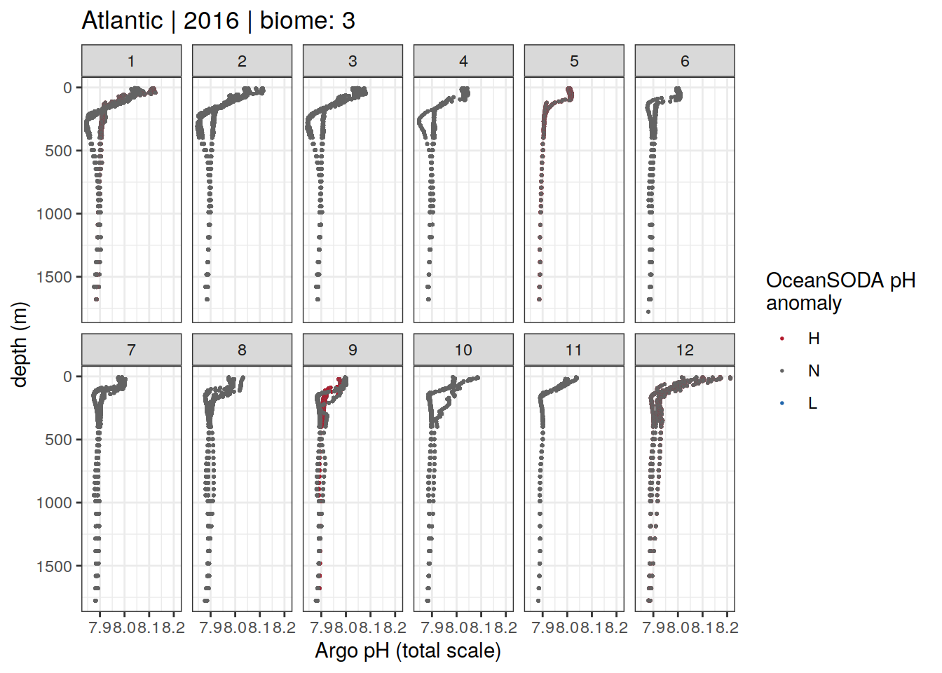
[[44]]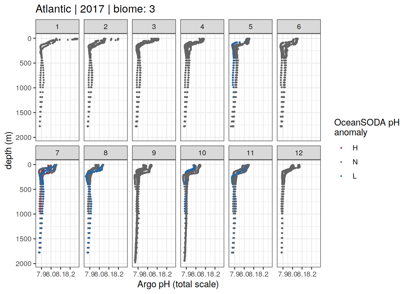
[[45]]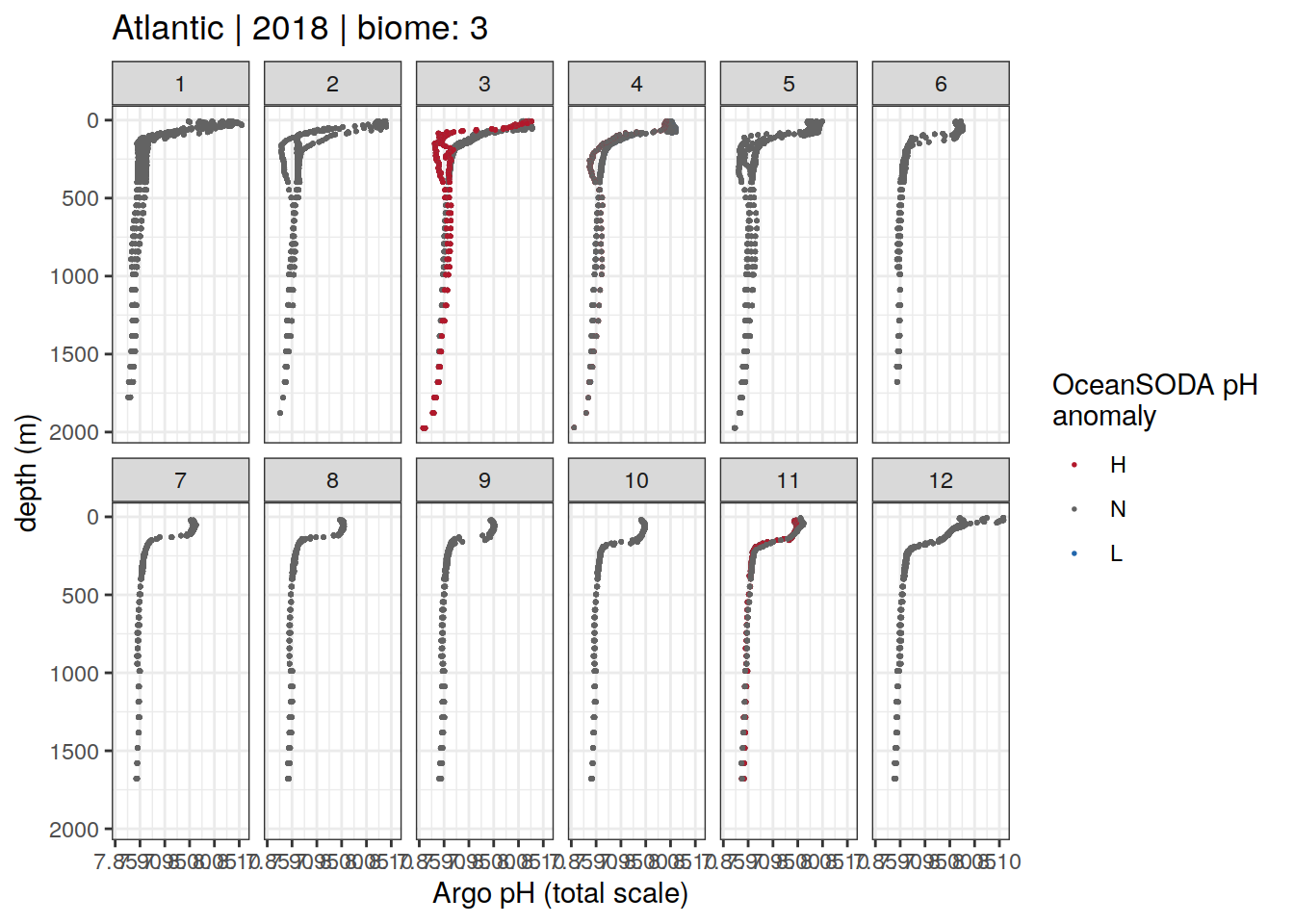
[[46]]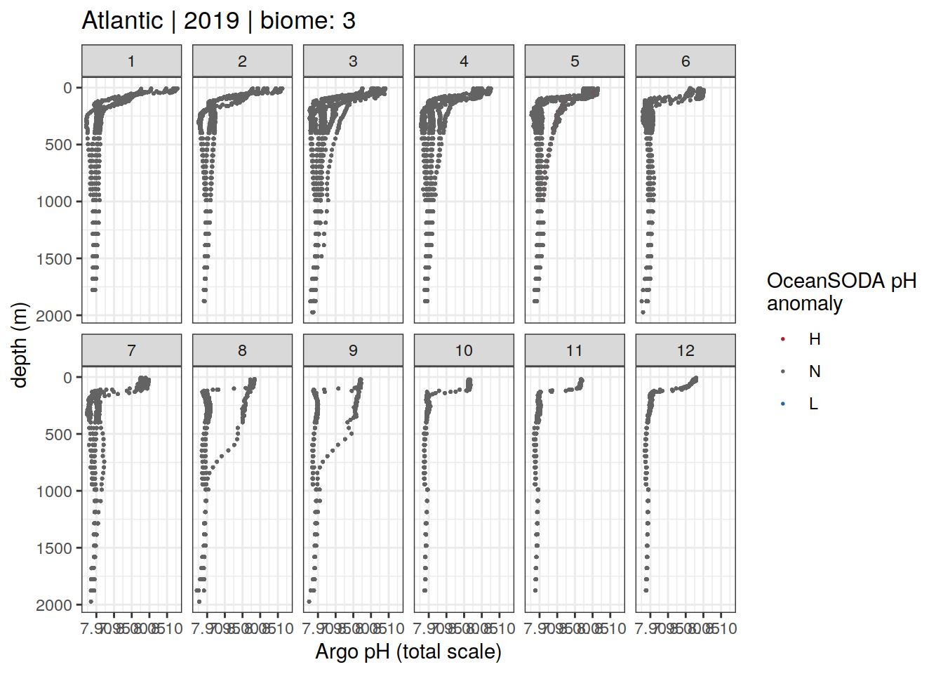
[[47]]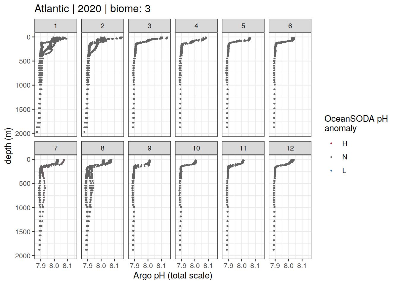
[[48]]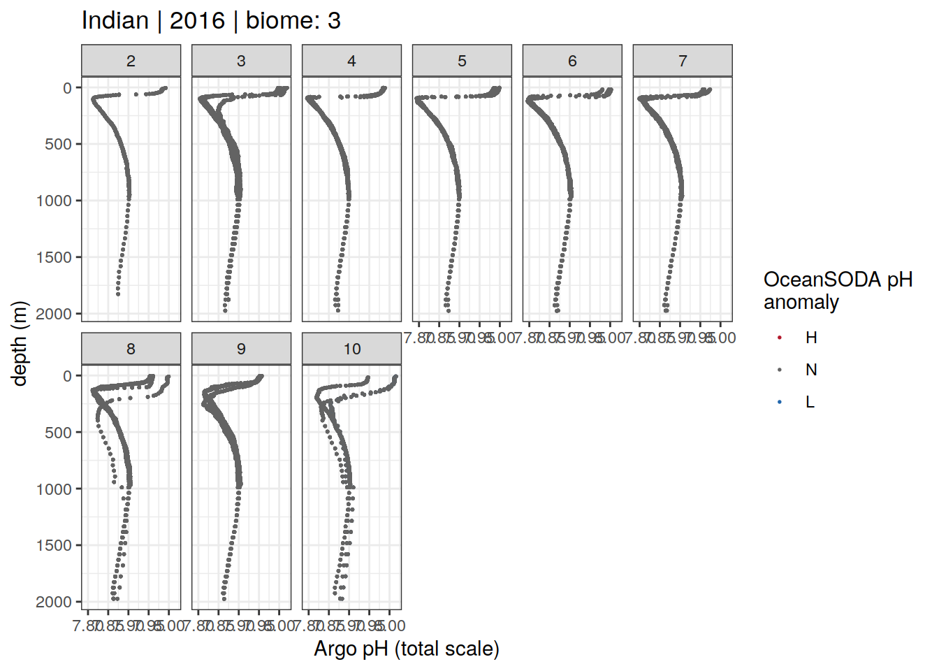
[[49]]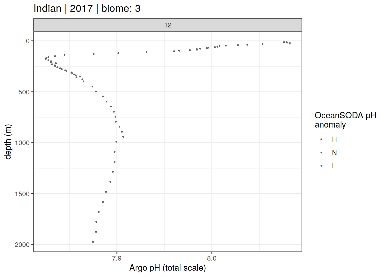
[[50]]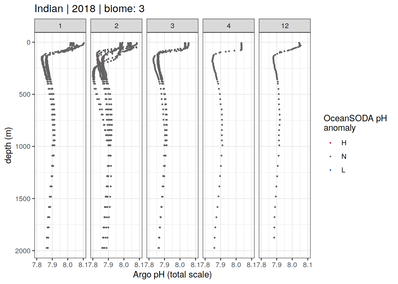
[[51]]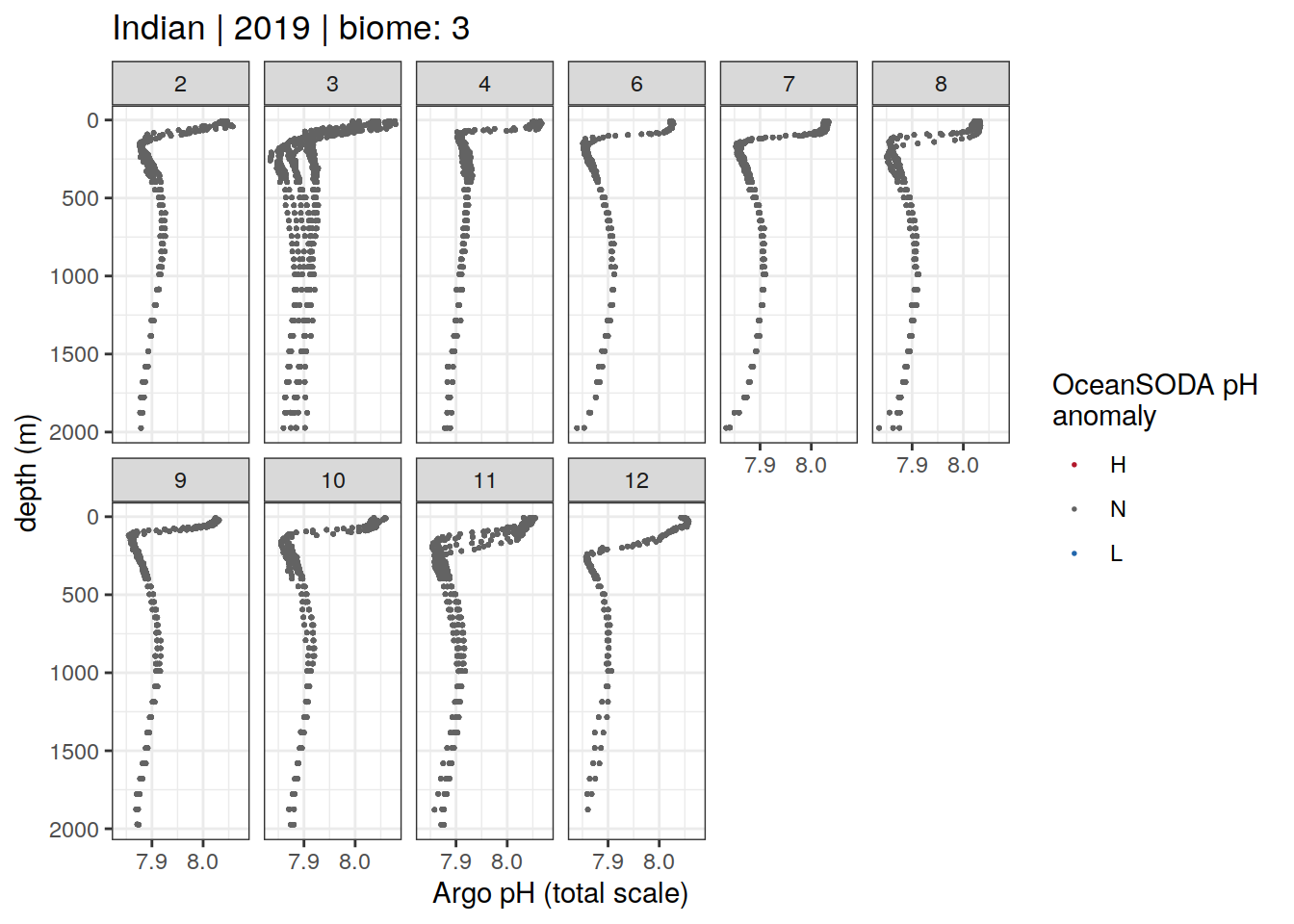
[[52]]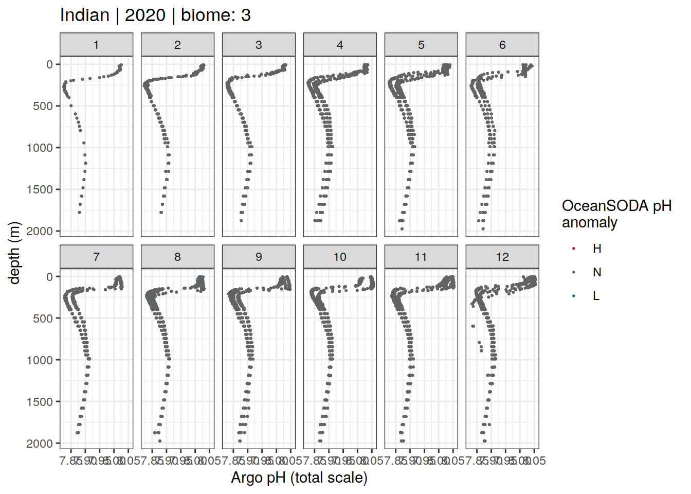
[[53]]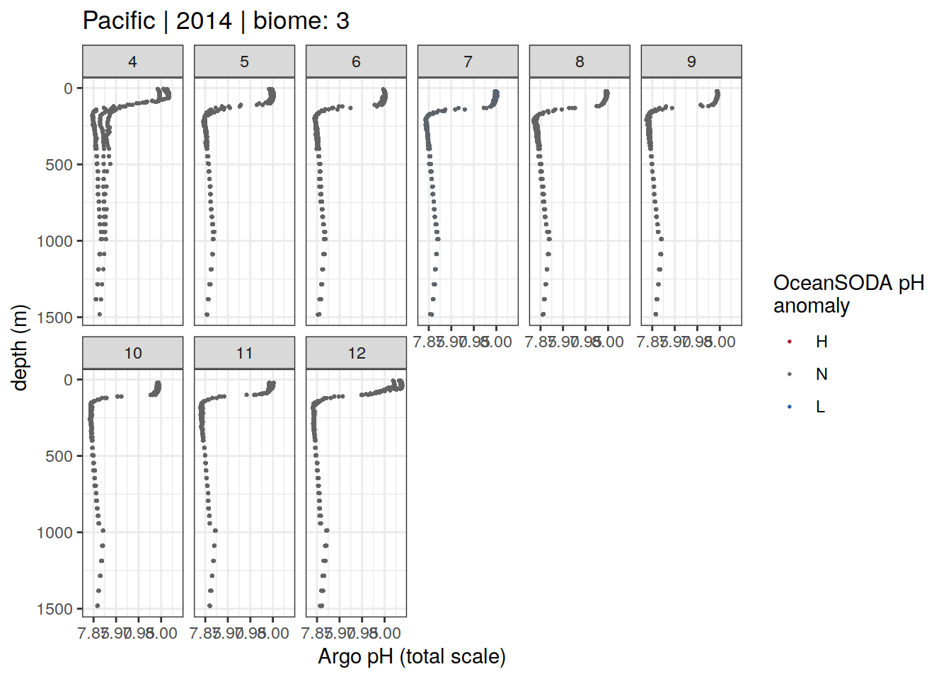
[[54]]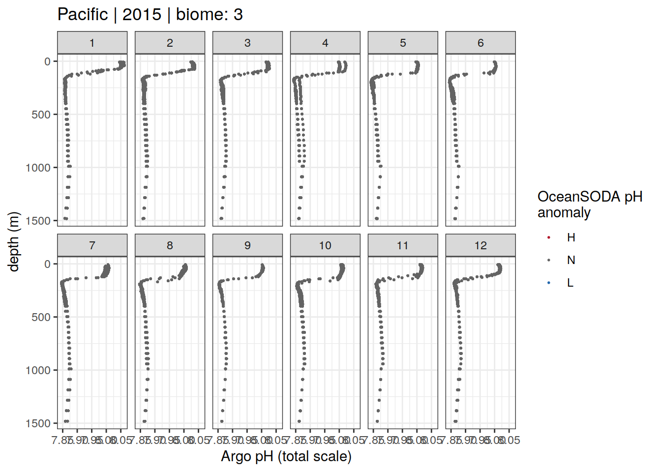
[[55]]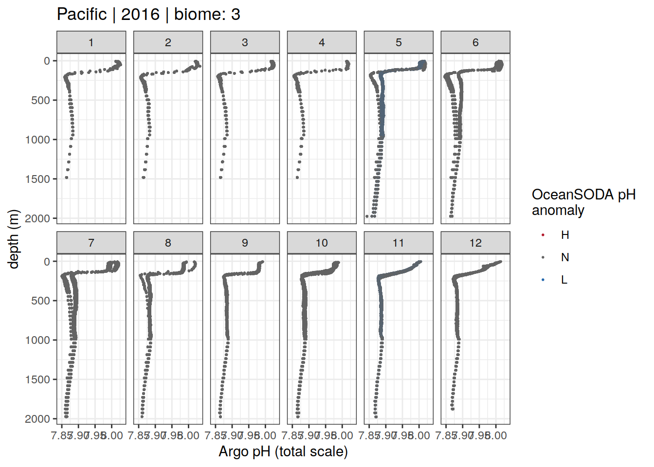
[[56]]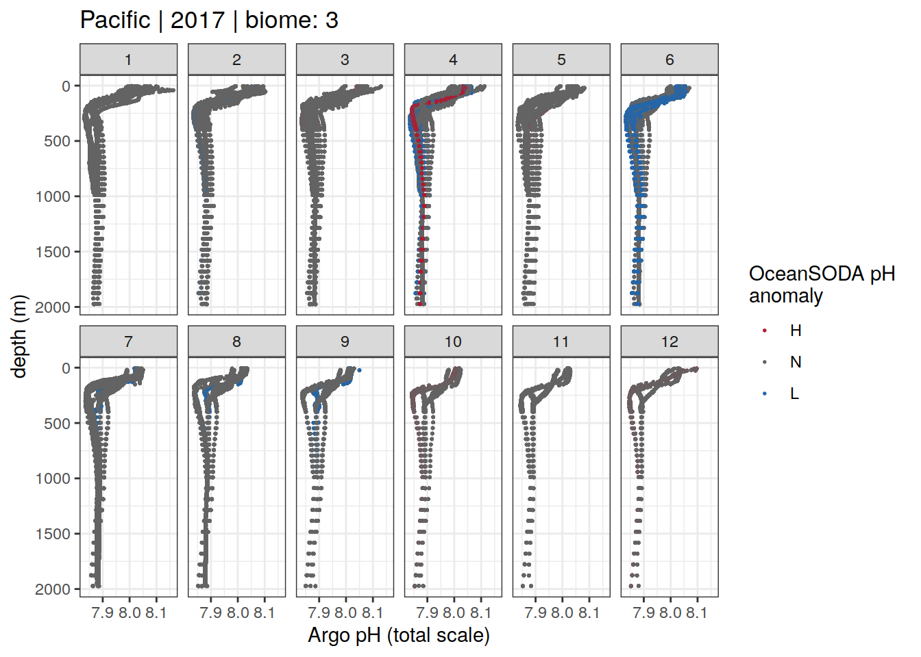
[[57]]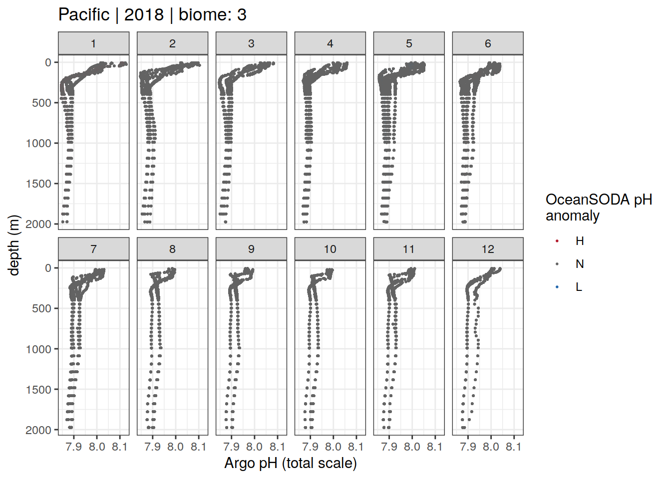
[[58]]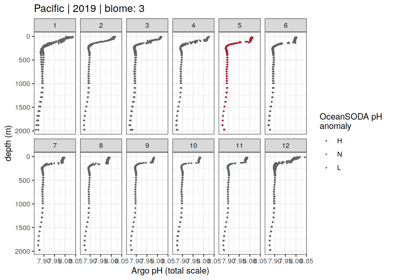
[[59]]
Temperature
# # plot temperature profiles for the Atlantic
# profile_extreme %>%
#   group_split(biome, basin_AIP, year) %>%
#   # head(1) %>%
#   map(
#     ~ ggplot(
#       data = .x,
#       aes(
#         x = temp_adjusted,
#         y = depth,
#         group = ph_extreme,
#         col = ph_extreme
#       )
#     ) +
#       geom_point(pch = 19, size = 0.5) +
#       scale_y_reverse() +
#       scale_color_manual(values = HNL_colors) +
#       facet_wrap( ~ month, ncol = 6) +
#       labs(
#         x = 'Argo temperature (°C)',
#         y = 'depth (m)',
#         title = paste(
#           unique(.x$basin_AIP),
#           "|",
#           unique(.x$year),
#           "| biome:",
#           unique(.x$biome)
#         ),
#         col = 'OceanSODA\npH\nanomaly'
#       )
#   )
Plot monthly profiles
# calculate mean profiles in each basin and biome, for each month between 2014 and 2021
# cut depth levels at 10, 20, .... etc m
# add seasons
# Dec, Jan, Feb <- summer
# Mar, Apr, May <- autumn
# Jun, Jul, Aug <- winter
# Sep, Oct, Nov <- spring

profile_extreme_monthly <- profile_extreme %>%
  mutate(depth = Hmisc::cut2(depth,
                             cuts = c(10, 20, 30, 50, 70, 100, 300, 500, 800, 1000, 1500, 2000, 2500),
                             m = 5,
                             levels.mean = TRUE),
         depth = as.numeric(as.character(depth))) %>%
  mutate(season = case_when(
    between(month, 3, 5) ~ 'autumn',
    between(month, 6, 8) ~ 'winter',
    between(month, 9, 11) ~ 'spring',
    month == 12 | 1 | 2 ~ 'summer'),
    .after = date
  ) %>%
  group_by(season, biome, basin_AIP, ph_extreme, depth) %>%
  summarise(ph_mean = mean(ph_in_situ_total_adjusted, na.rm = TRUE),
            temp_mean = mean(temp_adjusted, na.rm = TRUE)) %>%
  ungroup()
pH
By season
profile_extreme_monthly %>%
  arrange(depth) %>%
  group_split(season) %>%
  # head(1) %>%
  map(
    ~ ggplot(data = .x,
             aes(
               x = ph_mean,
               y = depth,
               group = ph_extreme,
               col = ph_extreme
             )) +
      geom_path() +
      scale_color_manual(values = HNL_colors) +
      labs(title = paste("season:", unique(.x$season)),
           col = 'OceanSODA\npH\nanomaly') +
      scale_y_reverse() +
      facet_grid(basin_AIP ~ biome)
  )
[[1]]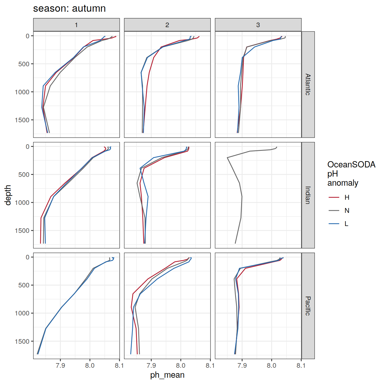
| Version | Author | Date |
|---|---|---|
| 962cdb9 | pasqualina-vonlanthendinenna | 2022-01-25 |
[[2]]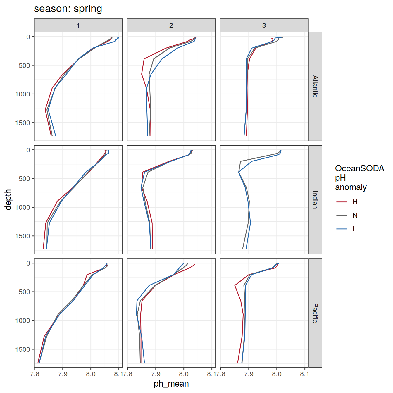
| Version | Author | Date |
|---|---|---|
| 962cdb9 | pasqualina-vonlanthendinenna | 2022-01-25 |
[[3]]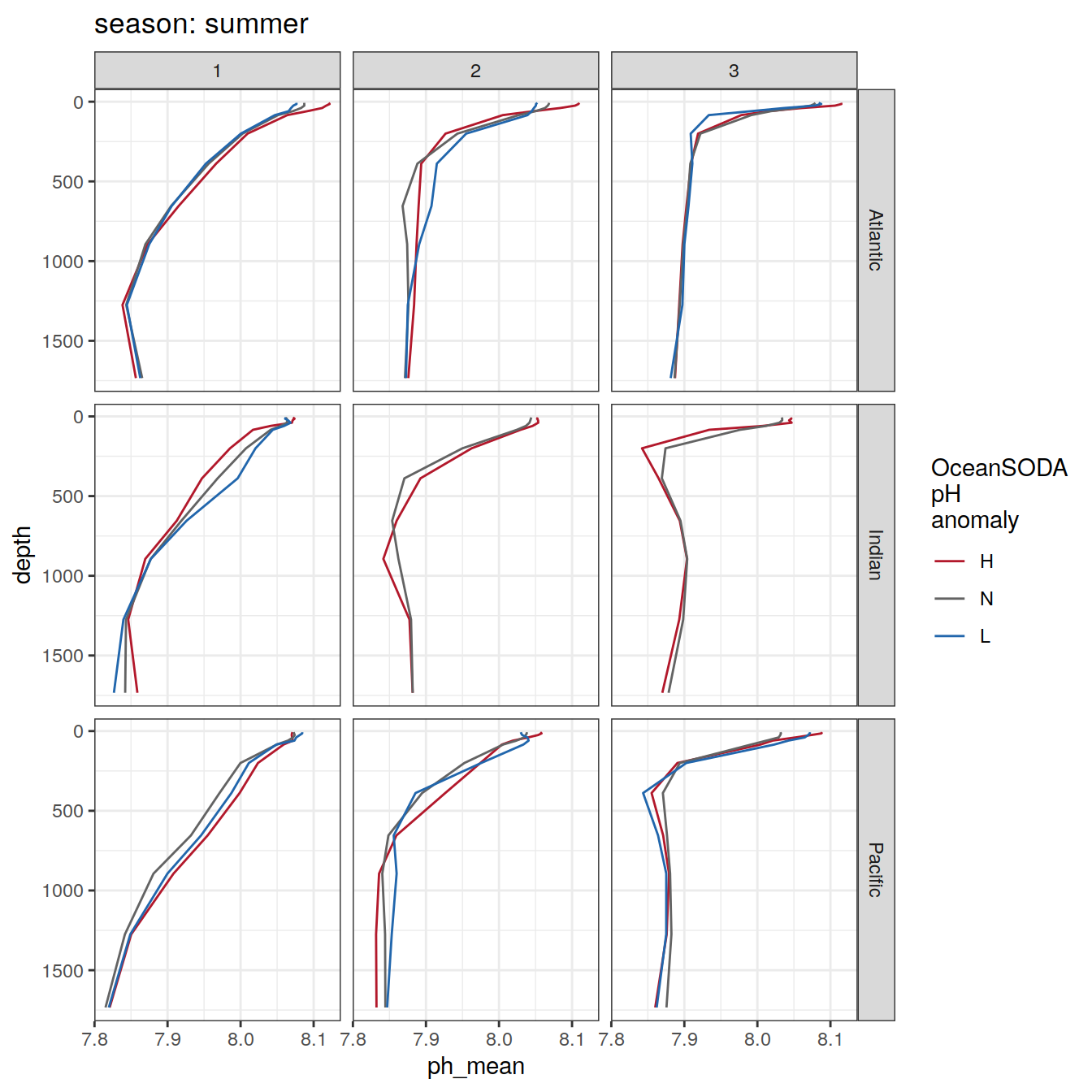
| Version | Author | Date |
|---|---|---|
| 962cdb9 | pasqualina-vonlanthendinenna | 2022-01-25 |
[[4]]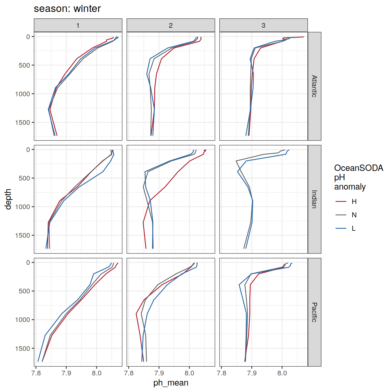
| Version | Author | Date |
|---|---|---|
| 962cdb9 | pasqualina-vonlanthendinenna | 2022-01-25 |
Averaged over biomes
profile_extreme_biome <- profile_extreme_monthly %>%
  group_by(season, biome, ph_extreme, depth) %>%
  summarise(ph_biome = mean(ph_mean, na.rm = TRUE)) %>%
  ungroup()


profile_extreme_biome %>%
  ggplot(aes(x = ph_biome,
                y = depth,
                group = ph_extreme,
                col = ph_extreme))+
  geom_path()+
  scale_color_manual(values = HNL_colors)+
  labs(col = 'OceanSODA\npH\nanomaly')+
  scale_y_reverse()+
  facet_grid(season ~ biome)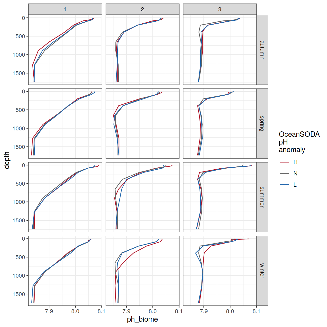
| Version | Author | Date |
|---|---|---|
| 962cdb9 | pasqualina-vonlanthendinenna | 2022-01-25 |
Averaged over ocean basins
profile_extreme_basin <- profile_extreme_monthly %>%
  group_by(season, basin_AIP, ph_extreme, depth) %>%
  summarise(ph_basin = mean(ph_mean, na.rm = TRUE)) %>%
  ungroup()

profile_extreme_basin %>%
  ggplot(aes(x = ph_basin,
             y = depth,
             group = ph_extreme,
             col = ph_extreme))+
  geom_path()+
  scale_color_manual(values = HNL_colors)+
  labs(col = 'OceanSODA\npH\nanomaly')+
  scale_y_reverse()+
  facet_grid(season~basin_AIP)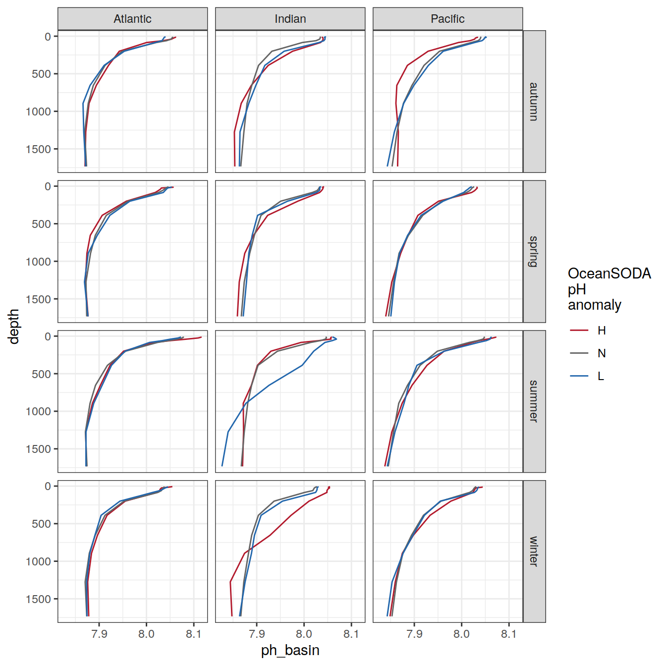
sessionInfo()R version 4.1.2 (2021-11-01)
Platform: x86_64-pc-linux-gnu (64-bit)
Running under: openSUSE Leap 15.3
Matrix products: default
BLAS: /usr/local/R-4.1.2/lib64/R/lib/libRblas.so
LAPACK: /usr/local/R-4.1.2/lib64/R/lib/libRlapack.so
locale:
[1] LC_CTYPE=en_US.UTF-8 LC_NUMERIC=C
[3] LC_TIME=en_US.UTF-8 LC_COLLATE=en_US.UTF-8
[5] LC_MONETARY=en_US.UTF-8 LC_MESSAGES=en_US.UTF-8
[7] LC_PAPER=en_US.UTF-8 LC_NAME=C
[9] LC_ADDRESS=C LC_TELEPHONE=C
[11] LC_MEASUREMENT=en_US.UTF-8 LC_IDENTIFICATION=C
attached base packages:
[1] stats graphics grDevices utils datasets methods base
other attached packages:
[1] ggOceanMaps_1.2.6 ggspatial_1.1.5 broom_0.7.11 lubridate_1.8.0
[5] forcats_0.5.1 stringr_1.4.0 dplyr_1.0.7 purrr_0.3.4
[9] readr_2.1.1 tidyr_1.1.4 tibble_3.1.6 ggplot2_3.3.5
[13] tidyverse_1.3.1 workflowr_1.7.0
loaded via a namespace (and not attached):
[1] colorspace_2.0-2 ellipsis_0.3.2 class_7.3-20
[4] rgdal_1.5-28 rprojroot_2.0.2 htmlTable_2.4.0
[7] base64enc_0.1-3 fs_1.5.2 rstudioapi_0.13
[10] proxy_0.4-26 farver_2.1.0 bit64_4.0.5
[13] fansi_1.0.2 xml2_1.3.3 codetools_0.2-18
[16] splines_4.1.2 knitr_1.37 Formula_1.2-4
[19] jsonlite_1.7.3 cluster_2.1.2 dbplyr_2.1.1
[22] png_0.1-7 rgeos_0.5-9 ggOceanMapsData_1.0.1
[25] compiler_4.1.2 httr_1.4.2 backports_1.4.1
[28] assertthat_0.2.1 Matrix_1.4-0 fastmap_1.1.0
[31] cli_3.1.1 later_1.3.0 htmltools_0.5.2
[34] tools_4.1.2 gtable_0.3.0 glue_1.6.0
[37] Rcpp_1.0.8 cellranger_1.1.0 jquerylib_0.1.4
[40] raster_3.5-11 vctrs_0.3.8 xfun_0.29
[43] ps_1.6.0 rvest_1.0.2 lifecycle_1.0.1
[46] terra_1.5-12 getPass_0.2-2 scales_1.1.1
[49] vroom_1.5.7 hms_1.1.1 promises_1.2.0.1
[52] parallel_4.1.2 RColorBrewer_1.1-2 yaml_2.2.1
[55] gridExtra_2.3 sass_0.4.0 rpart_4.1-15
[58] latticeExtra_0.6-29 stringi_1.7.6 highr_0.9
[61] checkmate_2.0.0 e1071_1.7-9 rlang_0.4.12
[64] pkgconfig_2.0.3 evaluate_0.14 lattice_0.20-45
[67] sf_1.0-5 htmlwidgets_1.5.4 labeling_0.4.2
[70] bit_4.0.4 processx_3.5.2 tidyselect_1.1.1
[73] magrittr_2.0.1 R6_2.5.1 generics_0.1.1
[76] Hmisc_4.6-0 DBI_1.1.2 pillar_1.6.4
[79] haven_2.4.3 whisker_0.4 foreign_0.8-82
[82] withr_2.4.3 units_0.7-2 survival_3.2-13
[85] sp_1.4-6 nnet_7.3-17 modelr_0.1.8
[88] crayon_1.4.2 KernSmooth_2.23-20 utf8_1.2.2
[91] tzdb_0.2.0 rmarkdown_2.11 jpeg_0.1-9
[94] grid_4.1.2 readxl_1.3.1 data.table_1.14.2
[97] callr_3.7.0 git2r_0.29.0 reprex_2.0.1
[100] digest_0.6.29 classInt_0.4-3 httpuv_1.6.5
[103] munsell_0.5.0 bslib_0.3.1