Core-Argo Temperature Data North Atlantic
Marguerite Larriere & Jens Daniel Müller
13 April, 2024
Last updated: 2024-04-13
Checks: 7 0
Knit directory:
bgc_argo_r_argodata/analysis/
This reproducible R Markdown analysis was created with workflowr (version 1.7.0). The Checks tab describes the reproducibility checks that were applied when the results were created. The Past versions tab lists the development history.
Great! Since the R Markdown file has been committed to the Git repository, you know the exact version of the code that produced these results.
Great job! The global environment was empty. Objects defined in the global environment can affect the analysis in your R Markdown file in unknown ways. For reproduciblity it’s best to always run the code in an empty environment.
The command set.seed(20211008) was run prior to running
the code in the R Markdown file. Setting a seed ensures that any results
that rely on randomness, e.g. subsampling or permutations, are
reproducible.
Great job! Recording the operating system, R version, and package versions is critical for reproducibility.
Nice! There were no cached chunks for this analysis, so you can be confident that you successfully produced the results during this run.
Great job! Using relative paths to the files within your workflowr project makes it easier to run your code on other machines.
Great! You are using Git for version control. Tracking code development and connecting the code version to the results is critical for reproducibility.
The results in this page were generated with repository version e2b710d. See the Past versions tab to see a history of the changes made to the R Markdown and HTML files.
Note that you need to be careful to ensure that all relevant files for
the analysis have been committed to Git prior to generating the results
(you can use wflow_publish or
wflow_git_commit). workflowr only checks the R Markdown
file, but you know if there are other scripts or data files that it
depends on. Below is the status of the Git repository when the results
were generated:
Ignored files:
    Ignored:    .Rproj.user/

Unstaged changes:
    Modified:   analysis/_site.yml
    Modified:   analysis/load_broullon_DIC_TA_clim.Rmd
    Modified:   code/Workflowr_project_managment.R
    Modified:   code/start_background_job.R
    Modified:   code/start_background_job_load.R
    Modified:   code/start_background_job_partial.R
Note that any generated files, e.g. HTML, png, CSS, etc., are not included in this status report because it is ok for generated content to have uncommitted changes.
These are the previous versions of the repository in which changes were
made to the R Markdown
(analysis/coverage_maps_North_Atlantic.Rmd) and HTML
(docs/coverage_maps_North_Atlantic.html) files. If you’ve
configured a remote Git repository (see ?wflow_git_remote),
click on the hyperlinks in the table below to view the files as they
were in that past version.
| File | Version | Author | Date | Message |
|---|---|---|---|---|
| html | c076fba | mlarriere | 2024-04-12 | Build site. |
| Rmd | a52cee0 | mlarriere | 2024-04-08 | adding subsection MHWs categorisation |
| html | bb83082 | mlarriere | 2024-04-08 | Build site. |
| Rmd | 8c713e2 | mlarriere | 2024-04-08 | cleaning code |
| html | d892578 | mlarriere | 2024-04-08 | Build site. |
| Rmd | 5876cbb | mlarriere | 2024-04-08 | cleaning code |
| html | 91f08a6 | mlarriere | 2024-04-07 | Build site. |
| html | db21f55 | mlarriere | 2024-04-06 | Build site. |
| Rmd | 5627ad6 | mlarriere | 2024-04-04 | until coverage_maps_North_Atlantic building test |
Task
Dependencies
temp_core_va.rds - core preprocessed folder, created by temp_core_align_climatology. Not this file is written AFTER the vertical alignment stage.
Outputs
path_emlr_utilities <- "/nfs/kryo/work/jenmueller/emlr_cant/utilities/files/"
path_basin_mask <- "/nfs/kryo/work/datasets/gridded/ocean/interior/reccap2/supplementary/"
path_argo <- '/nfs/kryo/work/datasets/ungridded/3d/ocean/floats/bgc_argo'
path_argo_core <- '/nfs/kryo/work/datasets/ungridded/3d/ocean/floats/core_argo_r_argodata_2024-03-13'

path_argo_core_preprocessed <- paste0(path_argo_core, "/preprocessed_core_data")
path_argo_preprocessed <- paste0(path_argo, "/preprocessed_bgc_data")
Set options
# Options

# opt_profile_depth_range
# The profile must have at least one temperature reading at a depth <= opt_profile_depth_range[1, ]
# The profile must have at least one temperature reading at a depth >= opt_profile_depth_range[2, ].
# In addition if the profile depth does not exceed the min(opt_profile_depth_range[2, ]) (i.e. 600) it will be removed.
profile_range <- c(1, 2, 3)
min_depth <- c(5.0, 5.0, 5.0)
max_depth <- c(600, 1200, 1500)
opt_profile_depth_range <- data.frame(profile_range, min_depth, max_depth)

# The profile should not have a gap greater that opt_gap_limit within the range defined by opt_gap_min_depth and opt_gap_max_depth
opt_gap_limit <- c(28, 55, 110)
opt_gap_min_depth <- c(0, 400, 1000)
opt_gap_max_depth <- c(400, 1000, 1500)

# year to be refreshed are set by opt_min_year and opt_max_year
opt_min_year = 2013
opt_max_year = 2024

# opt_measure_label, opt_xlim and opt_xbreaks are associated with formatting
opt_measure_label <- "temperature anomaly (°C)"
opt_xlim <- c(-4.5, 6)
opt_xbreaks <- c(-4, -2, 0, 2, 4, 6)

# opt_exclude_shallower
# This option will exclude depths from the climatology and subsequent vertically aligned data that are shallower than opt_exclude_shallower.
# e.g. set to 4.5 to ensure that the top depth of 0.0 m is excluded
# Set to 0.0 to ensure no depths are excluded.
opt_exclude_shallower <- 4.5
RECCAP biomes
#Load biome separations
region_masks_all <-
  stars::read_ncdf(paste(
    path_basin_mask, "RECCAP2_region_masks_all_v20221025.nc", sep = "")) %>%
  as_tibble() %>%
  mutate(seamask = as.factor(seamask))

#Select Atlantic
region_masks_atlantic <- region_masks_all %>%
  mutate(lon = ifelse(lon > 180, lon - 360, lon)) %>% #shift longitude to be in range (-180°, 180°) for better vizualisation
  pivot_longer(open_ocean:atlantic,
               names_to = 'region',
               values_to = 'value') %>%
  mutate(value = as.factor(value))


#Base map
# map <- read_rds(paste(path_emlr_utilities, "map_landmask_WOA18.rds", sep = ""))
world_coordinates <- map_data("world")

base_map <-ggplot() +
  geom_map(data = world_coordinates, map = world_coordinates,
    aes(long, lat, map_id = region))

#Restrict base map to North Atlantic Ocean
base_map <- base_map + lims(x= c(-100, 50), y = c(0, 80))

region_masks_atlantic <- region_masks_atlantic %>%
  filter(region == 'atlantic',
         value != 0) %>%
  mutate(coast = as.character(coast))
Coastal regions
#Map coastal regions
base_map +  geom_tile(data = region_masks_atlantic,
            aes(x = lon,
                y = lat,
                fill = coast)) +
  scale_fill_brewer(palette = 'Dark2')+
  labs(title = 'Coastal Regions')
Biomes
#Map biomes of interest:
      # SPSS (SubPolar Seasonally Stratified)
      # STSS (SubTropical Seasonally Stratified)
      # STPS (SubTropical Permanent Stratified)

biomes_names<-c("SPSS", "STSS", "STPS")

biomes_atlantic <- region_masks_atlantic %>%
  filter(value %in% c(1,2,3))

base_map + geom_tile(data = biomes_atlantic,
            aes(x = lon,
                y = lat,
                fill = value))+
  scale_fill_manual(values = c("1" = "cadetblue", "2" = "azure", "3" = "lightskyblue3"),
                    labels = biomes_names) +
  labs(title = 'RECCAP biomes')
Load Core-SST data
# Temperature profile in 2023
sst <- read_rds(file = paste0(path_argo_core_preprocessed, "/temp_core_va.rds")) %>%
  filter(year==2023) %>%
  mutate(lon = ifelse(lon > 180, lon - 360, lon))

# North Atlantic SST
sst_natlantic <- sst %>%
  group_by(year, file_id, lat, lon, profile_range) %>%
  filter(lat > 0, lon <30, lon >-100)

biomes_subset <- biomes_atlantic %>%
  select(lat, lon, biome_value = value)

sst_with_biomes <- left_join(sst, biomes_subset, by = c("lat", "lon")) %>%
  select(-date) %>%
  filter(!is.na(biome_value))
Functions
map_profiles<-function(data, by_year=FALSE, all_years=FALSE){
  # Number of measurements
  measurement_count <- data %>%
    group_by(year, file_id, lat, lon, profile_range) %>%
    summarise(count_measures = n()) %>%
    ungroup()

  # Number of profiles
  profile_count <- measurement_count %>%
    group_by(year, lat, lon, profile_range) %>%
    summarise(count_profiles = n()) %>%
    ungroup()

  # Aggregate profile range (only up to 600m depth)
  profile_count_agg <- profile_count %>%
    group_by(year, lat, lon) %>%
    summarise(count_profiles = sum(count_profiles)) %>%
    mutate(profile_range = 1) %>%
    ungroup()

  #Type of measurement
  profile_count_agg <- profile_count_agg %>%
    mutate (prof_type = 'temperature')

  if (by_year){
    map <- profile_count_agg %>%
      group_split(profile_range) %>%
      map(~ base_map +
            geom_tile(data = .x, aes(x = lon, y = lat, fill = count_profiles)) +
            scale_fill_gradient(low = "blue", high = "red", trans = "log10") +
            labs(x = 'lon', y = 'lat', fill = 'number of\nprofiles',
                 title = paste0('Core temperature by year and location ',
                                ifelse(unique(.x$profile_range) == 1, '600m'),
                                ' profiles')) +
            theme(legend.position = "bottom",
                  axis.text = element_blank(),
                  axis.ticks = element_blank()) +
            facet_wrap(~year, ncol = 3))
  }

  if (all_years){
    # sum across year
    profile_count_agg <- profile_count_agg %>%
      group_by(profile_range, lat, lon) %>%
      summarise(count_profiles = sum(count_profiles)) %>%
      ungroup()

    # map the location of profiles for each profile in each year
    map <- profile_count_agg %>%
      group_split(profile_range) %>%
      map(~ base_map +
            geom_tile(data = .x, aes(x = lon, y = lat, fill = count_profiles)) +
            scale_fill_gradient(low = "blue", high = "red", trans = "log10") +
            labs(x = 'lon', y = 'lat', fill = 'number of\nprofiles',
                 title = paste0('Core temperature by location ',
                                ifelse(unique(.x$profile_range) == 1, '600m',
                                       ifelse(unique(.x$profile_range) == 2, '1200m', '1500m')),
                                'profiles')) +
            theme(legend.position = "bottom",
                  axis.text = element_blank(),
                  axis.ticks = element_blank())
          )
  }

  return(map)

}
map_profiles_biomes<-function(data, by_biome=FALSE, map=FALSE, hist=FALSE){
# Number of measurements
measurement_count <- data %>%
group_by(year, file_id, lat, lon, profile_range, biome_value) %>%
summarise(count_measures = n()) %>%
ungroup()
# Number of profiles
profile_count <- measurement_count %>%
group_by(year, lat, lon, profile_range, biome_value) %>%
summarise(count_profiles = n()) %>%
ungroup()
# Aggregate profile range (only up to 600m)
profile_count_agg <- profile_count %>%
group_by(year, lat, lon, biome_value) %>%
summarise(count_profiles = sum(count_profiles)) %>%
mutate(profile_range = 1) %>%
ungroup()
#Type of measurement
profile_count_agg <- profile_count_agg %>%
mutate (prof_type = 'temperature')
if (by_biome){
# sum across biomes
profile_count_agg <- profile_count_agg %>%
group_by(lat, lon,profile_range, biome_value) %>%
summarise(count_profiles = sum(count_profiles)) %>%
ungroup()
if(map){
# map the location of profiles for each profile in each year
map <- base_map +
geom_tile(data = profile_count_agg, aes(x = lon, y = lat, fill = count_profiles)) +
scale_fill_gradient(low = "blue", high = "red", trans = "log10") +
labs(x = 'lon', y = 'lat', fill = 'number of\nprofiles',
title = 'Core temperature by biome profiles') +
theme(legend.position = "bottom",
axis.text = element_blank(),
axis.ticks = element_blank()) +
facet_wrap(~biome_value, ncol = 3, labeller = as_labeller(c(`1` = 'SPSS', `2` = 'STSS', `3` = 'STPS')))
return(map)
}
if (hist){
hist <- ggplot(profile_count_agg, aes(x = factor(biome_value), y = count_profiles, fill = factor(profile_range))) +
geom_bar(stat = "identity") +
labs(x = "Biome", y = "Number of Profiles", fill = "Profile Range") +
scale_fill_manual(values = c("1" = "orange"),
labels = c("1" = "600m")) +
theme_minimal() +
scale_x_discrete(labels = c("1" = "SPSS", "2" = "STSS", "3" = "STPS"))
return(hist)
}
}
}hist_profiles_months<-function(data){
# Number of measurements
measurement_count <- data %>%
group_by(month, year, file_id, lat, lon, biome_value) %>%
summarise(count_measures = n()) %>%
ungroup()
# Number of profiles
profile_count <- measurement_count %>%
group_by(month, year, lat, lon, biome_value) %>%
summarise(count_profiles = n()) %>%
ungroup()
# Aggregate profile range
profile_count_agg <- profile_count %>%
group_by(month, year, lat, lon, biome_value) %>%
summarise(count_profiles = sum(count_profiles)) %>%
ungroup()
#Type of measurement
profile_count_agg <- profile_count_agg %>%
mutate (prof_type = 'temperature')
# sum across biomes
profile_count_agg <- profile_count_agg %>%
group_by(month, lat, lon, biome_value) %>%
summarise(count_profiles = sum(count_profiles)) %>%
ungroup()
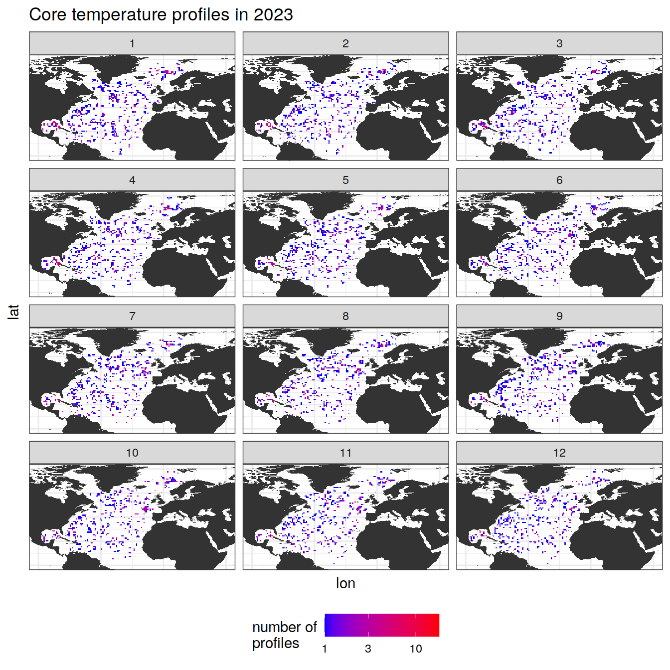
hist <- ggplot(profile_count_agg, aes(x = factor(month), y = count_profiles, fill = factor(biome_value))) +
geom_bar(stat = "identity") +
labs(title= paste0("Number of profiles per month, per biome, in 2023"), x = "Biome", y = "Number of Profiles", fill = "Profile Range") +
scale_fill_manual(values = c("1" = "lightblue", "2" = "orange", "3" = "darkred"),
labels = c("1" = "SPSS", "2" = "STSS", "3" = "STPS")) +
theme_minimal()
return(hist)
}map_profiles_months<-function(data, by_year=FALSE, all_years=FALSE){
# Number of measurements
measurement_count <- data %>%
group_by(month, year, file_id, lat, lon) %>%
summarise(count_measures = n()) %>%
ungroup()
# Number of profiles
profile_count <- measurement_count %>%
group_by(month, year, lat, lon) %>%
summarise(count_profiles = n()) %>%
ungroup()
# Aggregate profile range
profile_count_agg <- profile_count %>%
group_by(month, year, lat, lon) %>%
summarise(count_profiles = sum(count_profiles)) %>%
ungroup()
#Type of measurement
profile_count_agg <- profile_count_agg %>%
mutate (prof_type = 'temperature')
if (by_year){
map <- base_map +
geom_tile(data =profile_count_agg, aes(x = lon, y = lat, fill = count_profiles)) +
scale_fill_gradient(low = "blue", high = "red", trans = "log10") +
labs(x = 'lon', y = 'lat', fill = 'number of\nprofiles',
title = 'Core temperature profiles in 2023')+
theme(legend.position = "bottom",
axis.text = element_blank(),
axis.ticks = element_blank()) +
facet_wrap(~month, ncol = 3)
}
if (all_years){
# sum across year
profile_count_agg <- profile_count_agg %>%
group_by(lat, lon) %>%
summarise(count_profiles = sum(count_profiles)) %>%
ungroup()
# map the location of profiles for each profile in each year
map <- profile_count_agg %>%
map(~ base_map +
geom_tile(data = .x, aes(x = lon, y = lat, fill = count_profiles)) +
scale_fill_gradient(low = "blue", high = "red", trans = "log10") +
labs(x = 'lon', y = 'lat', fill = 'number of\nprofiles',
title = 'Core temperature profiles over years') +
theme(legend.position = "bottom",
axis.text = element_blank(),
axis.ticks = element_blank())
)
}
return(map)
}Profiles spatial distribution
By year
# Map the location of profiles for each profile in each year
map_profiles(sst_natlantic, by_year = TRUE)
[[1]]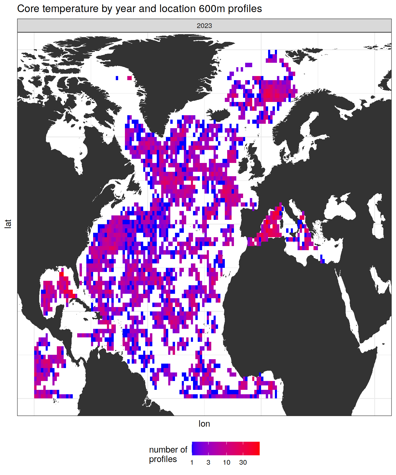
Over all years
# Map the location of profiles over all years
map_profiles(sst_natlantic, by_year = FALSE, all_years = TRUE)
By biomes over all years
# Map the location of profiles over all years, per biomes
map_profiles_biomes(sst_with_biomes, by_biome=TRUE, map=TRUE, hist = FALSE)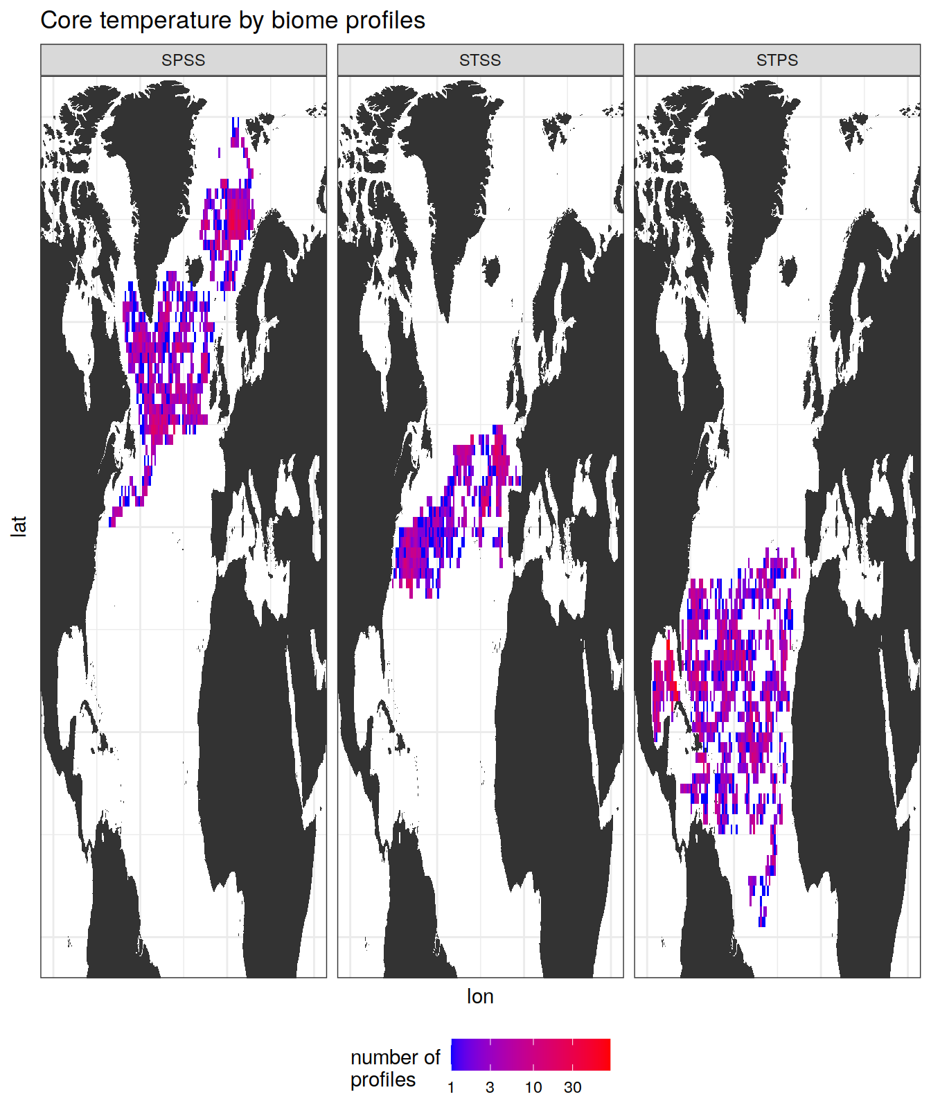
# Number of profiles over all years, per biomes
map_profiles_biomes(sst_with_biomes, by_biome=TRUE, map=FALSE, hist = TRUE)
Histogram number of profiles per year, per months
# Map the location of profiles over all years, per biomes
hist_profiles_months(sst_with_biomes)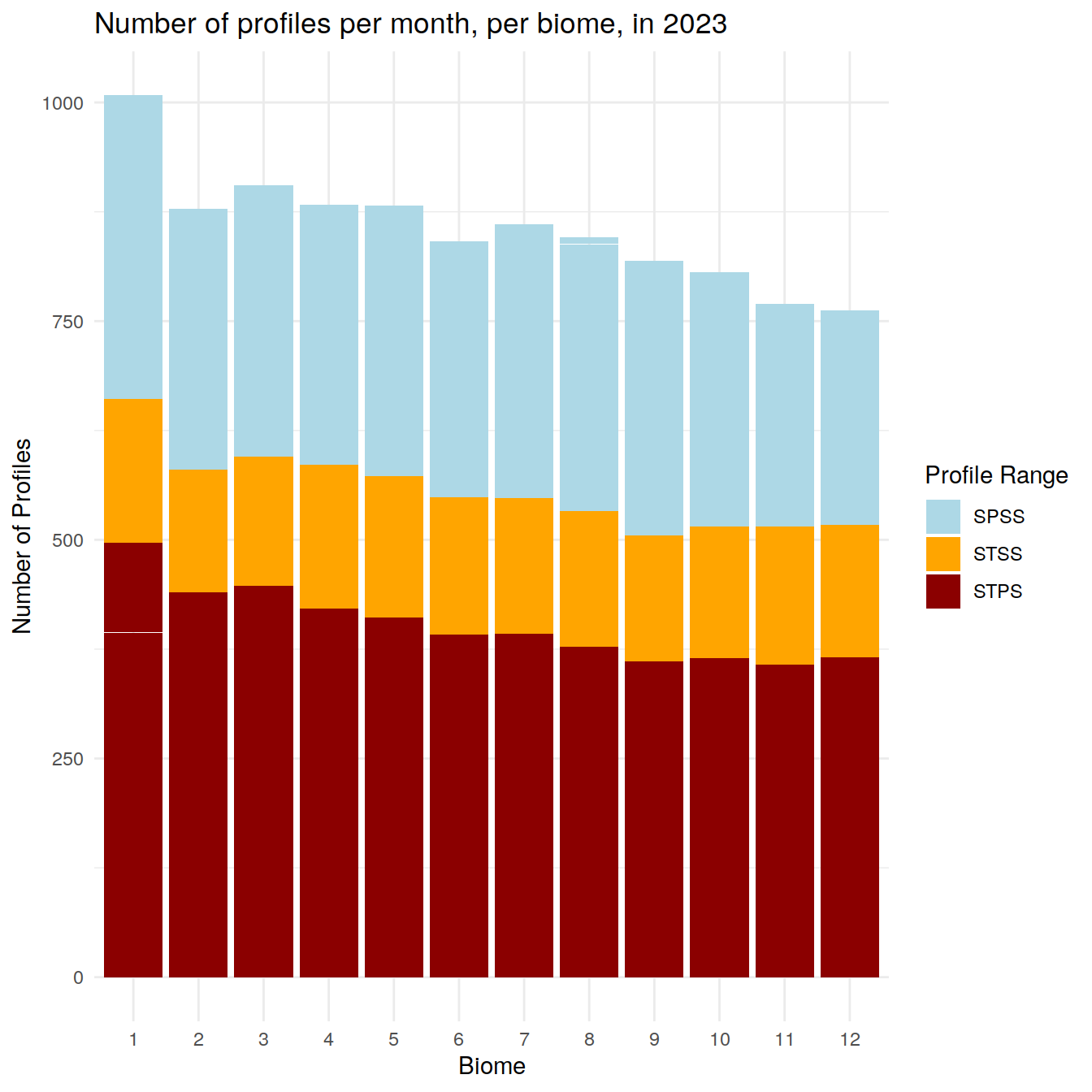
Anomaly profiles for each biomes
Load anomaly datasets
# Temperature profile
temp_anomaly_va <- read_rds(file = paste0(path_argo_core_preprocessed, "/temp_anomaly_va.rds")) %>%
  filter(year==2023) %>%
  mutate(lon = ifelse(lon > 180, lon - 360, lon))

# North Atlantic SST
temp_anomaly_va_natlantic <- temp_anomaly_va %>%
  group_by(year, file_id, lat, lon, profile_range) %>%
  filter(lat > 0, lon <30, lon >-100)

temp_anomaly_va_biomes <- left_join(temp_anomaly_va_natlantic, biomes_subset, by = c("lat", "lon")) %>%
  select(-date) %>%
  filter(!is.na(biome_value))
plot_anomaly_profiles <- function(data, max_depth) {
anomaly_overall_mean <- data %>%
filter(depth <= max_depth) %>%
group_by(depth) %>%
summarise(temp_count = n(),
temp_anomaly_mean = mean(anomaly, na.rm = TRUE),
temp_anomaly_sd = sd(anomaly, na.rm = TRUE))
ggplot(anomaly_overall_mean) +
geom_path(aes(x = temp_anomaly_mean, y = depth)) +
geom_ribbon(aes(xmax = temp_anomaly_mean + temp_anomaly_sd,
xmin = temp_anomaly_mean - temp_anomaly_sd,
y = depth), alpha = 0.2) +
geom_vline(xintercept = 0) +
scale_y_reverse() +
coord_cartesian(xlim = opt_xlim) +
scale_x_continuous(breaks = opt_xbreaks) +
labs(title = paste0('North Atlantic (all biomes) mean anomaly profiles to ', max_depth, 'm', ""),
x = opt_measure_label, y = 'depth (m)')
}# Profiles to 600m
max_depth_1 <- opt_profile_depth_range[1, "max_depth"]
plot_anomaly_profiles(temp_anomaly_va_natlantic, max_depth_1)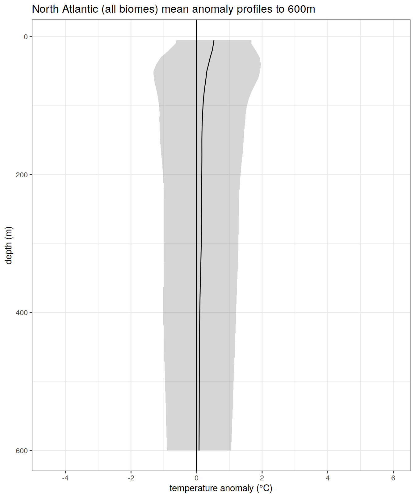
# Profiles to 1200m
# max_depth_2 <- opt_profile_depth_range[2, "max_depth"]
# plot_anomaly_profiles(temp_anomaly_va_natlantic, max_depth_2)

# Profiles to 1500m
# max_depth_3 <- opt_profile_depth_range[3, "max_depth"]
# plot_anomaly_profiles(temp_anomaly_va_natlantic, max_depth_3)
plot_anomaly_profiles_biomes <- function(data, max_depth, group_monthly=FALSE) {
if (group_monthly) {
anomaly_overall_mean <- data %>%
filter(depth <= max_depth) %>%
group_by(depth, biome_value, month) %>%
summarise(temp_count = n(),
temp_anomaly_mean = mean(anomaly, na.rm = TRUE),
temp_anomaly_sd = sd(anomaly, na.rm = TRUE))
facet_var <- ~ month
labeller <- as_labeller(setNames(month.name[1:12], as.character(1:12)))
} else {
anomaly_overall_mean <- data %>%
filter(depth <= max_depth) %>%
group_by(depth, biome_value) %>%
summarise(temp_count = n(),
temp_anomaly_mean = mean(anomaly, na.rm = TRUE),
temp_anomaly_sd = sd(anomaly, na.rm = TRUE))
facet_var <- ~ factor(biome_value)
labeller <- as_labeller(c("1" = "SPSS", "2" = "STSS", "3" = "STPS"))
}
ggplot(anomaly_overall_mean) +
geom_path(aes(x = temp_anomaly_mean, y = depth, color = factor(biome_value))) +
geom_ribbon(aes(xmax = temp_anomaly_mean + temp_anomaly_sd,
xmin = temp_anomaly_mean - temp_anomaly_sd,
y = depth, fill = factor(biome_value)), alpha = 0.2) +
geom_vline(xintercept = 0) +
scale_y_reverse() +
coord_cartesian(xlim = opt_xlim) +
scale_x_continuous(breaks = opt_xbreaks) +
labs(title = paste0('Mean anomaly (per biome) profiles to ', max_depth, 'm', ""),
x = opt_measure_label, y = 'depth (m)', color = "Biome") +
scale_color_manual(values = c("1" = "darkblue", "2" = "darkorange", "3" = "darkred"), labels = c("SPSS", "STSS", "STPS")) +
scale_fill_manual(values = c("1" = "darkblue", "2" = "darkorange", "3" = "darkred"), name = "Biome", labels = c("SPSS", "STSS", "STPS")) +
facet_wrap(facet_var, labeller = labeller, ncol = 3) +
theme(axis.text.x = element_text(angle = 0, hjust = 1))
}# Profiles to 600m
plot_anomaly_profiles_biomes(temp_anomaly_va_biomes, max_depth_1, group_monthly=FALSE)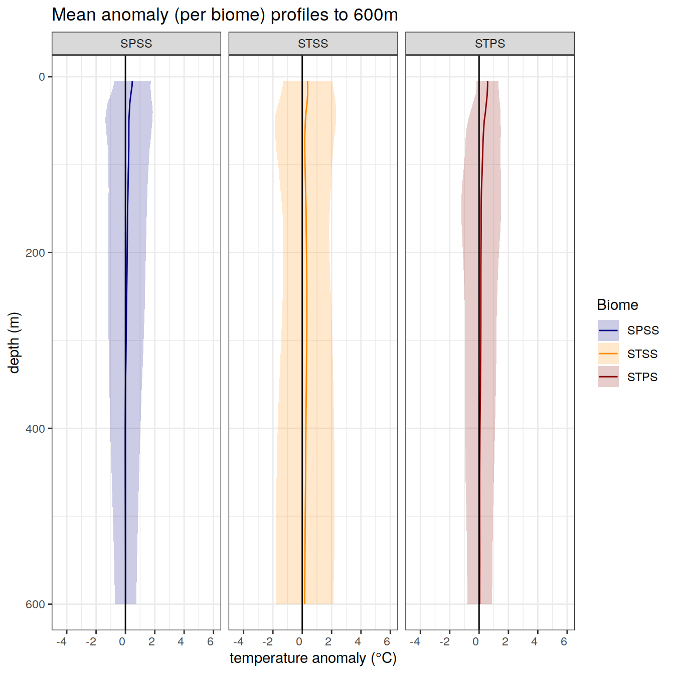
# Profiles to 1200m
# plot_anomaly_profiles_biomes(temp_anomaly_va_biomes, max_depth_2,  group_monthly=FALSE)

# Profiles to 1500m
# plot_anomaly_profiles_biomes(temp_anomaly_va_biomes, max_depth_3,  group_monthly=FALSE)

# Profile per month
plot_anomaly_profiles_biomes(temp_anomaly_va_biomes, max_depth_1,  group_monthly=TRUE) #600m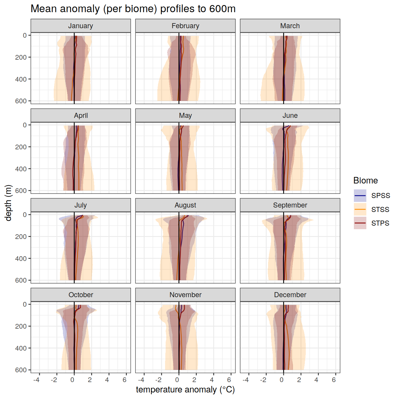
# plot_anomaly_profiles_biomes(temp_anomaly_va_biomes, max_depth_2,  group_monthly=TRUE) #1200m
# plot_anomaly_profiles_biomes(temp_anomaly_va_biomes, max_depth_3,  group_monthly=TRUE) #1500m
plot_anomaly_profiles_1month <- function(data, max_depth, month_of_interest) {
anomaly_overall_mean <- data %>%
filter(depth <= max_depth,
month == month_of_interest) %>%
group_by(depth, biome_value, month, year) %>%
summarise(temp_count = n(),
temp_anomaly_mean = mean(anomaly, na.rm = TRUE),
temp_anomaly_sd = sd(anomaly, na.rm = TRUE))
plot_date <- paste("Date:", month.name[unique(anomaly_overall_mean$month)], unique(anomaly_overall_mean$year))
ggplot(anomaly_overall_mean) +
geom_path(aes(x = temp_anomaly_mean, y = depth, color = factor(biome_value))) +
geom_ribbon(aes(xmax = temp_anomaly_mean + temp_anomaly_sd,
xmin = temp_anomaly_mean - temp_anomaly_sd,
y = depth, fill = factor(biome_value)), alpha = 0.2) +
geom_vline(xintercept = 0) +
scale_y_reverse() +
coord_cartesian(xlim = opt_xlim) +
scale_x_continuous(breaks = opt_xbreaks) +
labs(title = paste0('Overall mean anomaly profiles to ', max_depth, 'm', ""),
subtitle = plot_date,
x = opt_measure_label, y = 'depth (m)', color = "Biome") +
scale_color_manual(values = c("1" = "darkblue", "2" = "darkorange", "3" = "darkred"), labels = c("SPSS", "STSS", "STPS")) +
scale_fill_manual(values = c("1" = "darkblue", "2" = "darkorange", "3" = "darkred"), name = "Biome", labels = c("SPSS", "STSS", "STPS")) +
facet_wrap(~ month, ncol = 3)+
theme(axis.text.x = element_text(angle = 0, hjust = 1))
}# Profiles to 600m
plot_anomaly_profiles_1month(temp_anomaly_va_biomes, max_depth_1, month_of_interest=10)
# Profiles to 1200m
# plot_anomaly_profiles_1month(temp_anomaly_va_biomes, max_depth_2, month_of_interest=10)
# Profiles to 1500m
# plot_anomaly_profiles_1month(temp_anomaly_va_biomes, max_depth_3, month_of_interest=10)
#-- Focusing on specfific zone
temp_anomaly_va_biomes_zone<- temp_anomaly_va_biomes %>%
filter(lat<55, lat>40, lon > -65, lon < -35)
map_profiles_months(temp_anomaly_va_biomes_zone, by_year = TRUE)
plot_anomaly_profiles_1month(temp_anomaly_va_biomes_zone, max_depth_1, month_of_interest=9)
dev.off()
sessionInfo()R version 4.2.2 (2022-10-31)
Platform: x86_64-pc-linux-gnu (64-bit)
Running under: openSUSE Leap 15.5
Matrix products: default
BLAS: /usr/local/R-4.2.2/lib64/R/lib/libRblas.so
LAPACK: /usr/local/R-4.2.2/lib64/R/lib/libRlapack.so
locale:
[1] LC_CTYPE=en_US.UTF-8 LC_NUMERIC=C
[3] LC_TIME=en_US.UTF-8 LC_COLLATE=en_US.UTF-8
[5] LC_MONETARY=en_US.UTF-8 LC_MESSAGES=en_US.UTF-8
[7] LC_PAPER=en_US.UTF-8 LC_NAME=C
[9] LC_ADDRESS=C LC_TELEPHONE=C
[11] LC_MEASUREMENT=en_US.UTF-8 LC_IDENTIFICATION=C
attached base packages:
[1] stats graphics grDevices utils datasets methods base
other attached packages:
[1] ggOceanMaps_1.3.4 ggspatial_1.1.7 oce_1.7-10 gsw_1.1-1
[5] lubridate_1.9.0 timechange_0.1.1 forcats_0.5.2 stringr_1.5.0
[9] dplyr_1.1.3 purrr_1.0.2 readr_2.1.3 tidyr_1.3.0
[13] tibble_3.2.1 ggplot2_3.4.4 tidyverse_1.3.2 workflowr_1.7.0
loaded via a namespace (and not attached):
[1] fs_1.5.2 sf_1.0-9 httr_1.4.4
[4] rprojroot_2.0.3 tools_4.2.2 backports_1.4.1
[7] bslib_0.4.1 utf8_1.2.2 R6_2.5.1
[10] KernSmooth_2.23-20 rgeos_0.5-9 DBI_1.2.2
[13] colorspace_2.0-3 raster_3.6-11 sp_1.5-1
[16] withr_2.5.0 tidyselect_1.2.0 processx_3.8.0
[19] compiler_4.2.2 git2r_0.30.1 cli_3.6.1
[22] rvest_1.0.3 RNetCDF_2.6-1 xml2_1.3.3
[25] labeling_0.4.2 sass_0.4.4 scales_1.2.1
[28] classInt_0.4-8 callr_3.7.3 proxy_0.4-27
[31] digest_0.6.30 rmarkdown_2.18 pkgconfig_2.0.3
[34] htmltools_0.5.8.1 highr_0.9 maps_3.4.1
[37] dbplyr_2.2.1 fastmap_1.1.0 rlang_1.1.1
[40] readxl_1.4.1 rstudioapi_0.15.0 farver_2.1.1
[43] jquerylib_0.1.4 generics_0.1.3 jsonlite_1.8.3
[46] googlesheets4_1.0.1 magrittr_2.0.3 ncmeta_0.3.5
[49] Rcpp_1.0.10 munsell_0.5.0 fansi_1.0.3
[52] abind_1.4-5 lifecycle_1.0.3 terra_1.7-65
[55] stringi_1.7.8 whisker_0.4 yaml_2.3.6
[58] grid_4.2.2 parallel_4.2.2 promises_1.2.0.1
[61] crayon_1.5.2 lattice_0.20-45 stars_0.6-0
[64] haven_2.5.1 hms_1.1.2 knitr_1.41
[67] ps_1.7.2 pillar_1.9.0 codetools_0.2-18
[70] reprex_2.0.2 glue_1.6.2 evaluate_0.18
[73] getPass_0.2-2 modelr_0.1.10 vctrs_0.6.4
[76] tzdb_0.3.0 httpuv_1.6.6 cellranger_1.1.0
[79] gtable_0.3.1 assertthat_0.2.1 cachem_1.0.6
[82] xfun_0.35 lwgeom_0.2-10 broom_1.0.5
[85] e1071_1.7-12 later_1.3.0 class_7.3-20
[88] googledrive_2.0.0 gargle_1.2.1 units_0.8-0
[91] ellipsis_0.3.2 