Last updated: 2024-05-12

Checks: 7 0

Knit directory: bgc_argo_r_argodata/analysis/

This reproducible R Markdown analysis was created with workflowr (version 1.7.0). The Checks tab describes the reproducibility checks that were applied when the results were created. The Past versions tab lists the development history.

R Markdown file: up-to-date

Great! Since the R Markdown file has been committed to the Git repository, you know the exact version of the code that produced these results.

Environment: empty

Great job! The global environment was empty. Objects defined in the global environment can affect the analysis in your R Markdown file in unknown ways. For reproduciblity it’s best to always run the code in an empty environment.

Seed: set.seed(20211008)

The command set.seed(20211008) was run prior to running the code in the R Markdown file. Setting a seed ensures that any results that rely on randomness, e.g. subsampling or permutations, are reproducible.

Session information: recorded

Great job! Recording the operating system, R version, and package versions is critical for reproducibility.

Cache: none

Nice! There were no cached chunks for this analysis, so you can be confident that you successfully produced the results during this run.

File paths: relative

Great job! Using relative paths to the files within your workflowr project makes it easier to run your code on other machines.

Repository version: e52ed44

Great! You are using Git for version control. Tracking code development and connecting the code version to the results is critical for reproducibility.

The results in this page were generated with repository version e52ed44. See the Past versions tab to see a history of the changes made to the R Markdown and HTML files.

Note that you need to be careful to ensure that all relevant files for the analysis have been committed to Git prior to generating the results (you can use wflow_publish or wflow_git_commit). workflowr only checks the R Markdown file, but you know if there are other scripts or data files that it depends on. Below is the status of the Git repository when the results were generated:


Ignored files:
    Ignored:    .Rproj.user/
    Ignored:    analysis/figure/

Untracked files:
    Untracked:  analysis/draft.Rmd
    Untracked:  load_argo_core_output.txt

Unstaged changes:
    Modified:   analysis/_site.yml
    Modified:   analysis/child/cluster_analysis_base.Rmd
    Modified:   analysis/coverage_maps_North_Atlantic.Rmd
    Modified:   analysis/load_argo_core.Rmd
    Modified:   analysis/load_broullon_DIC_TA_clim.Rmd
    Modified:   analysis/temp_core_align_climatology.Rmd
    Modified:   code/Workflowr_project_managment.R
    Modified:   code/start_background_job.R
    Modified:   code/start_background_job_load.R
    Modified:   code/start_background_job_partial.R

Note that any generated files, e.g. HTML, png, CSS, etc., are not included in this status report because it is ok for generated content to have uncommitted changes.

These are the previous versions of the repository in which changes were made to the R Markdown (analysis/MHWs_categorisation.Rmd) and HTML (docs/MHWs_categorisation.html) files. If you’ve configured a remote Git repository (see ?wflow_git_remote), click on the hyperlinks in the table below to view the files as they were in that past version.

File	Version	Author	Date	Message
Rmd	e52ed44	mlarriere	2024-05-12	Anomaly profile east north atlantic - first try
html	ee73ee9	mlarriere	2024-05-12	Build site.
Rmd	80b57a8	mlarriere	2024-05-12	Anomaly profile east north atlantic - first try
html	af44bcd	mlarriere	2024-04-26	Build site.
html	07d81ba	mlarriere	2024-04-26	Build site.
Rmd	ca55ece	mlarriere	2024-04-26	Building test
html	bd8a25e	mlarriere	2024-04-26	Build site.
Rmd	bb7c075	mlarriere	2024-04-26	Building test
html	043a8d6	mlarriere	2024-04-25	Build site.
Rmd	e9d0c16	mlarriere	2024-04-25	Building test
html	f0289cd	mlarriere	2024-04-23	Build site.
Rmd	ae8003f	mlarriere	2024-04-23	Building test
html	0ada9ee	mlarriere	2024-04-22	Build site.
Rmd	fc5ac8c	mlarriere	2024-04-22	Adding SST anomaly subsection
html	83b6d9a	mlarriere	2024-04-22	Build site.
Rmd	40fff85	mlarriere	2024-04-22	Adding SST anomaly subsection
Rmd	4690882	mlarriere	2024-04-17	Elbow method graph and 2 clusters
html	924babc	mlarriere	2024-04-17	Build site.
Rmd	550ab72	mlarriere	2024-04-17	Cluster analysis test
html	4a8157c	mlarriere	2024-04-16	Build site.
Rmd	5acdc98	mlarriere	2024-04-16	Some explanations on categorisation and beginning of cluster analysis
html	ad0d737	mlarriere	2024-04-16	Build site.
Rmd	f22c4b5	mlarriere	2024-04-16	Some explanations on categorisation and beginning of cluster analysis
Rmd	2c60853	mlarriere	2024-04-15	Some explanations on categorisation and beginning of cluster analysis
html	9910de2	mlarriere	2024-04-14	Build site.
html	50596ee	mlarriere	2024-04-14	Build site.
Rmd	ac8de8b	mlarriere	2024-04-14	Figures MHWs
html	718d84b	mlarriere	2024-04-14	Build site.
Rmd	a2e118c	mlarriere	2024-04-14	Figures MHWs
html	c789e3f	mlarriere	2024-04-13	Build site.
Rmd	acdc838	mlarriere	2024-04-13	Figures MHWs
html	bbbc1bb	mlarriere	2024-04-13	Build site.
Rmd	b080fc9	mlarriere	2024-04-13	Figures MHWs
html	83d1fa3	mlarriere	2024-04-13	Build site.
Rmd	c8b3f67	mlarriere	2024-04-13	Figures MHWs
html	1ab66f1	mlarriere	2024-04-13	Build site.
Rmd	25928b0	mlarriere	2024-04-13	Figures MHWs
html	5475def	mlarriere	2024-04-13	Build site.
Rmd	e2b710d	mlarriere	2024-04-13	build North Atlanatic section
html	c076fba	mlarriere	2024-04-12	Build site.
Rmd	a52cee0	mlarriere	2024-04-08	adding subsection MHWs categorisation
html	efc6aab	mlarriere	2024-04-08	Build site.
Rmd	a9ea2a8	mlarriere	2024-04-08	test MHWs cat

Task

Focusing on 2023 Only core Argo - focus on temperature anomalies

Dependencies

temp_core_va.rds - temperature of core argo floats after vertical alignment.

core_metadata.rds - File with metadata concerning the floats such as platform number, cycle number, date, lat, lon and quality control results.

temp_anomaly_va.rds - file containing the temperature anomalies (temp core - climatology).

2023_mhw_raw.csv - CSV file containing the categorization of surface marine heatwaves, in 2023 and in a 0.25°x0.25° grid.

Outputs

2023_surface_mhws_1x1.rds - file containing the categorization of surface marine heatwaves in a 1°x1° grid, in 2023.

path_emlr_utilities <- "/nfs/kryo/work/jenmueller/emlr_cant/utilities/files/"
path_basin_mask <- "/nfs/kryo/work/datasets/gridded/ocean/interior/reccap2/supplementary/"
path_argo <- '/nfs/kryo/work/datasets/ungridded/3d/ocean/floats/bgc_argo'
path_argo_core <- '/nfs/kryo/work/datasets/ungridded/3d/ocean/floats/core_argo_r_argodata_2024-03-13'

path_argo_core_preprocessed <- paste0(path_argo_core, "/preprocessed_core_data")

path_mhw<- '/net/kryo/work/datasets/gridded/ocean/2d/obs/mhw'

opt_xbreaks <- c(-4, -2, 0, 2, 4)

# Define colors palette to match ~ color of ClimateReanalyser (for comparison)
colors <- c("lavender", "#9867C5", "darkblue", "lightblue", "white", "orange", "darkred", "red", "#FFCBCB")
palette <- colorRampPalette(colors)
n <- 20 #number of colors 
continuous_palette <- palette(n) #continuous color palette
scale_limits <- c(-10, 10)
scale_breaks <- seq(scale_limits[1], scale_limits[2], length.out = n + 1)

Load data

Load biomes

Load Argo floats data

Load SST anomaly

#Read SST anomaly, computed using climatology:2009-2019 (from anomaly_SST_2023.Rmd)
sst_anomaly_northAtlantic<- read_rds(paste(path_argo_core_preprocessed, "/SST_anomaly2023_NorthAtlantic_clim2004-2019.rds", sep = ""))

Argo floats

Distribution over entire North Atlantic basin

#Histogram -- number of floats per month and biome
unique_platforms_per_month <- core_anomaly_with_platform_2023 %>%
   group_by(month, biome_value) %>%
  filter(!is.na(biome_value)) %>% 
   summarize(unique_platforms = n_distinct(platform_number))

hist <- ggplot(unique_platforms_per_month, aes(x = factor(month), y = unique_platforms, fill=factor(biome_value))) +
      geom_bar(stat = "identity")+#, position = "dodge") +
      labs(title= paste0("Amount of platform per month and per biome, in 2023"), 
           x = "Months", y = "Number of argo floats", fill = "Biomes") +
      scale_fill_manual(values = c("1" = "#1034A6", "2" = "#f59c04", "3" = "darkred"),
                    labels = c("1" = "SPSS", "2" = "STSS", "3" = "STPS")) +
      theme_minimal()

print(hist)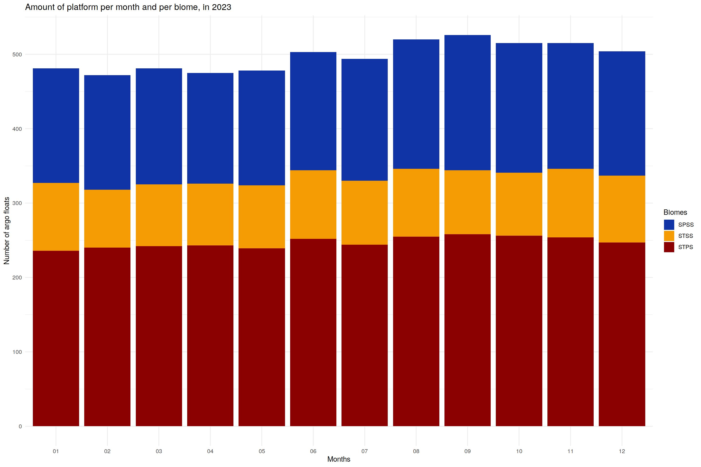

Version	Author	Date
ee73ee9	mlarriere	2024-05-12
0ada9ee	mlarriere	2024-04-22
83b6d9a	mlarriere	2024-04-22

#Number of cycle per platform
cycle_counts <- core_anomaly_with_platform_2023 %>%
  group_by(platform_number) %>%
  summarise(cycle_count = n_distinct(cycle_number))
print(cycle_counts)

# A tibble: 975 × 2
   platform_number cycle_count
   <chr>                 <int>
 1 1901711                  31
 2 1901728                  26
 3 1901730                  37
 4 1901731                  37
 5 1901820                   2
 6 1902070                   8
 7 1902073                  37
 8 1902180                  36
 9 1902181                  37
10 1902208                  37
# ℹ 965 more rows

Area of interest

Maps area of interest

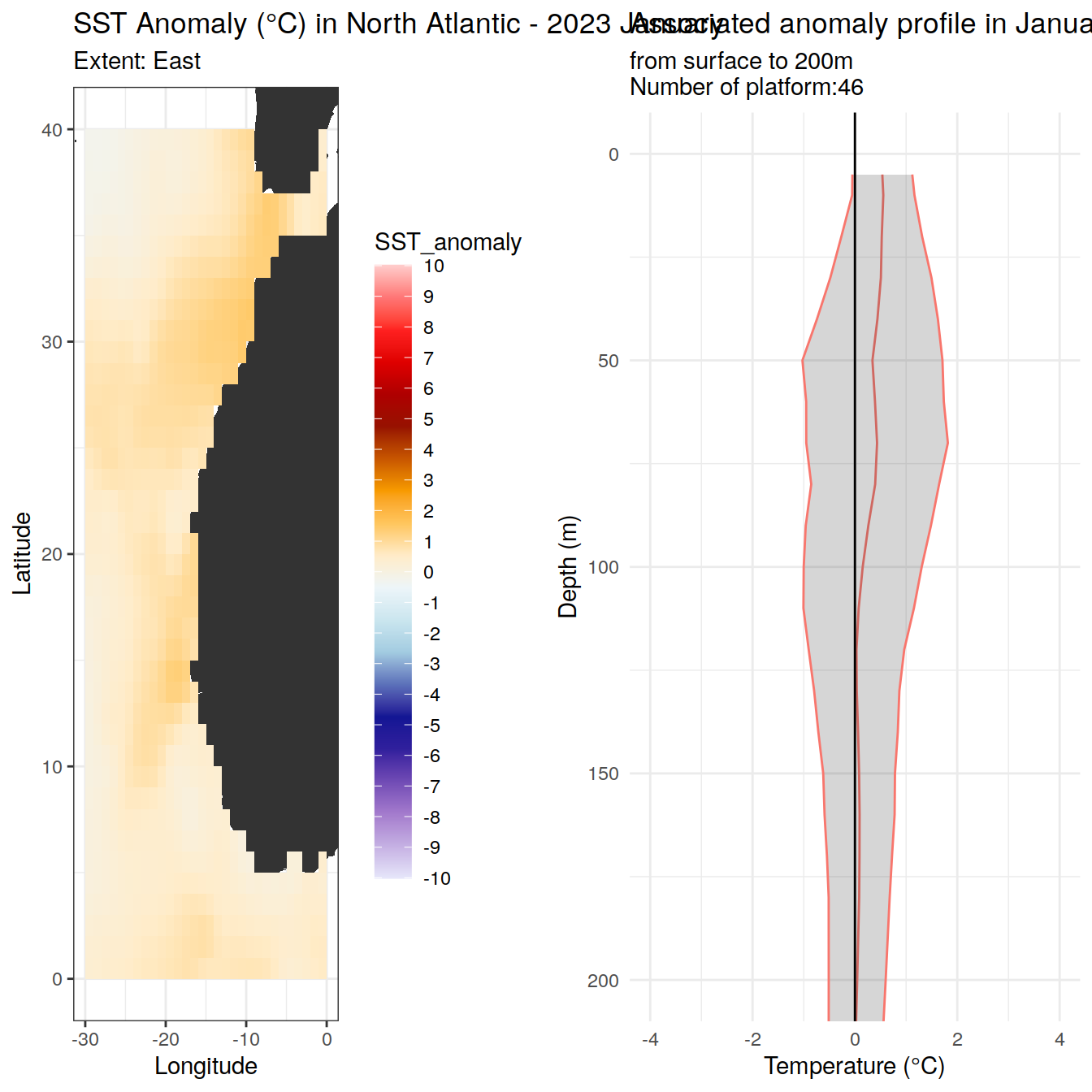
Using the SST map computed in “anomaly_SST_2023.Rmd” and ClimateReanalyser, we identify 2 areas of particular interest for SST anomalies in 2023 in the North Atlantic Ocean:

Northeast, near the Canada/USA coast. SST anomaly particularly strong in summer and autumn (JJA and SON).
East coast of the North Atlantic Ocean. Here, SST anomalies are high on an annual basis, with a sharp increase from June onwards.

Argo floats available

#Join the SST anomaly with the anomaly profiles
complete_anomaly_profile<- full_join(sst_anomaly_northAtlantic, core_anomaly_with_platform_2023, by=c("lat", "lon", "month"))

complete_anomaly_profile<-complete_anomaly_profile %>% 
  filter(!is.na(platform_number), !is.na(depth)) #remove profile where there is only SST anomaly and not deeper 

#Floats present during heatwaves
# East
heatwaves_data_east<-complete_anomaly_profile %>% 
  group_by(month) %>% 
  filter(lat>0, lat<40, lon>-30, 0>lon)

cycles_per_platform <-heatwaves_data_east %>%
  group_by(platform_number) %>%
  summarize(unique_cycles = toString(unique(cycle_number)))

months_per_float <- heatwaves_data_east %>%
  group_by(platform_number) %>%
  summarize(unique_months = toString(unique(month)))

platform_6903067<-heatwaves_data_east %>% 
  filter(platform_number==6903067)
custom_palette <- c("#1f77b4", "#ff7f0e", "#2ca02c", "#d62728", "#9467bd", "#8c564b",
                    "#e377c2", "#7f7f7f", "#bcbd22", "#17becf", "#aec7e8", "#ffbb78")
ggplot(platform_6903067, aes(x = anomaly, y = depth, color = factor(month))) +
  geom_path() +
  geom_vline(xintercept = 0) +
  scale_y_reverse() +
  coord_cartesian(xlim = c(-4, 4), ylim = c(200, 0)) +
  labs(title = 'Anomaly profiles by month',
       subtitle= '1 subplot per cycle',
       x = 'Temperature (°C)', y = 'Depth (m)', color = 'Month') +
  scale_color_manual(values = custom_palette) + 
  facet_wrap(~cycle_number, scales = "free_x", ncol = 5)

platform_6903067_base_map<- base_map + lims(x=c(-20,-10), y=c(10,20))

unique_coords_with_cycles <- platform_6903067 %>%
  distinct(lat, lon, .keep_all = TRUE) %>%
  group_by(lat, lon) %>%
  summarise(cycle_numbers = toString(unique(cycle_number)))

#base map and SST anomaly
map_anomaly_east <- platform_6903067_base_map + 
  geom_tile(data = east_sst_anomaly, aes(x = lon, y = lat, fill = SST_anomaly)) +
  scale_fill_gradientn(colors = continuous_palette, limits = scale_limits, breaks = scale_breaks) +
  labs(fill = "SST Anomaly") +
  theme_minimal()

#trajetory
map_anomaly_east + 
  geom_point(data = unique_coords_with_cycles, aes(x = lon, y = lat, color = cycle_numbers), size = 2) +
  scale_color_discrete(name = "Cycle Number", guide = guide_legend(title.position = "top")) +
  labs(title = 'Float position') +
  theme(legend.position = "bottom")+
    guides(fill = guide_colorbar(barwidth = 20, barheight = 1, title.position = "top"))

east_sst_anomaly<-sst_anomaly_northAtlantic %>% 
  filter(lat>0, lat<40, lon>-30, 0>lon)

cycles_per_platform_month<- heatwaves_data_east %>%
  group_by(platform_number, month) %>%
  summarize(unique_cycles = toString(unique(cycle_number)))

anomaly_mean <- heatwaves_data_east %>% 
  group_by(depth, month) %>% 
  summarise(temp_count = n(),
            temp_anomaly_mean = mean(anomaly, na.rm = TRUE),
            temp_anomaly_sd = sd(anomaly, na.rm = TRUE))
#For each mont put the SST anomaly next to the anomaly path
for (m in unique(east_sst_anomaly$month)) {
  # Filter data 
  map_data <- filter(east_sst_anomaly, month == m)
  anomaly_data <- filter(anomaly_mean, month == m)

  # Plot for temperature anomaly map
  map_plot <- east_base_map +
      geom_tile(data=map_data, aes(x = lon, y = lat, fill = SST_anomaly)) +
    scale_fill_gradientn(colors = continuous_palette,  limits = scale_limits, breaks = scale_breaks) +
    labs(title = paste("SST Anomaly (°C) in North Atlantic - 2023", month.name[as.numeric(m)]), 
         subtitle = "Extent: East",
         x = "Longitude", y = "Latitude") +
    theme(legend.position = 'right', legend.key.height = unit(2, "cm"))
  
  # Plot for anomaly profiles
  anomaly_plot <- ggplot(anomaly_data, aes(x = temp_anomaly_mean, y = depth, color = factor(month))) +
    geom_path() +
    geom_ribbon(aes(xmax = temp_anomaly_mean + temp_anomaly_sd,
                    xmin = temp_anomaly_mean - temp_anomaly_sd,
                    y = depth), alpha = 0.2) +
    geom_vline(xintercept = 0) +
    scale_y_reverse() +
    coord_cartesian(xlim = c(-4, 4), ylim = c(200, 0)) +
    scale_x_continuous(breaks = opt_xbreaks) +
    labs(title = paste('Associated anomaly profile in', month.name[as.numeric(m)]), 
         subtitle = paste0("from surface to 200m", "\nNumber of platform:",  nrow(filter(cycles_per_platform_month, month==m))),
         x = 'Temperature (°C)', y = 'Depth (m)') +
    theme_minimal()+
        guides(color = FALSE)

  
  #plots side by side
  combined_plot <- grid.arrange(map_plot, anomaly_plot, ncol = 2)
  print(combined_plot)
}

Version	Author	Date
ee73ee9	mlarriere	2024-05-12

TableGrob (1 x 2) "arrange": 2 grobs
  z     cells    name           grob
1 1 (1-1,1-1) arrange gtable[layout]
2 2 (1-1,2-2) arrange gtable[layout]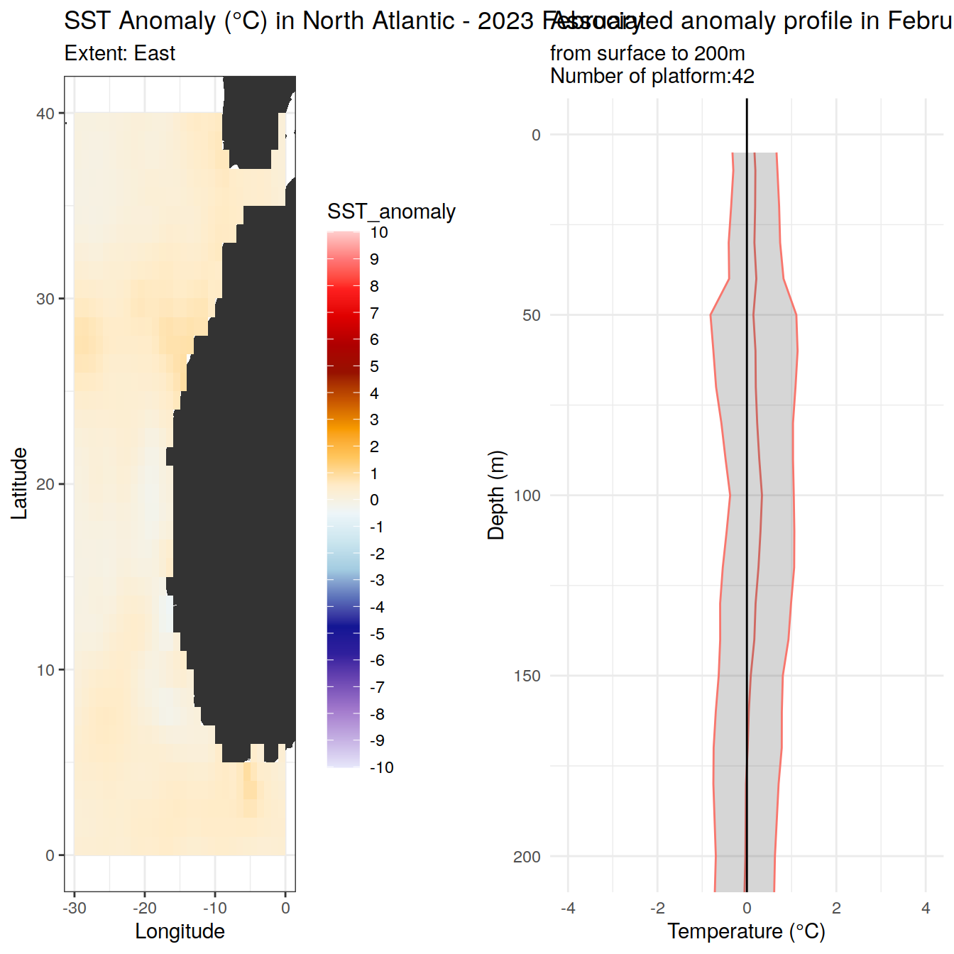

Version	Author	Date
ee73ee9	mlarriere	2024-05-12

TableGrob (1 x 2) "arrange": 2 grobs
  z     cells    name           grob
1 1 (1-1,1-1) arrange gtable[layout]
2 2 (1-1,2-2) arrange gtable[layout]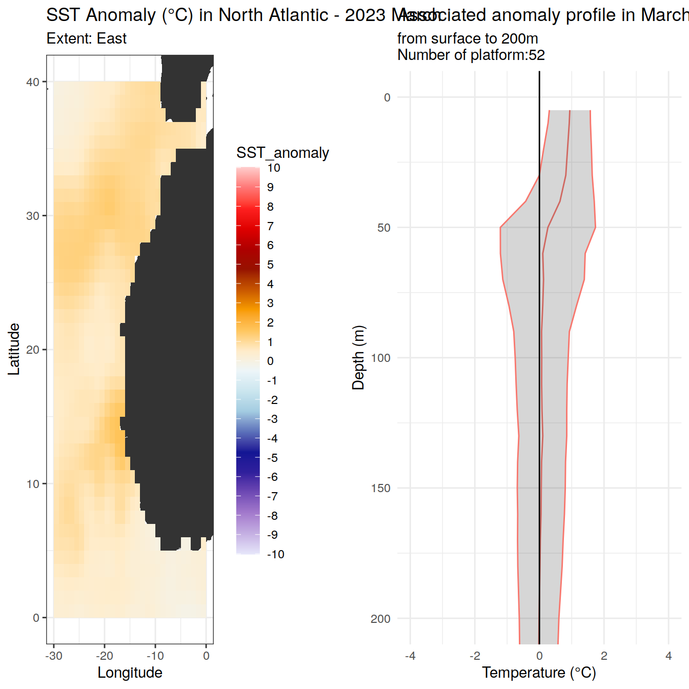

Version	Author	Date
ee73ee9	mlarriere	2024-05-12

TableGrob (1 x 2) "arrange": 2 grobs
  z     cells    name           grob
1 1 (1-1,1-1) arrange gtable[layout]
2 2 (1-1,2-2) arrange gtable[layout]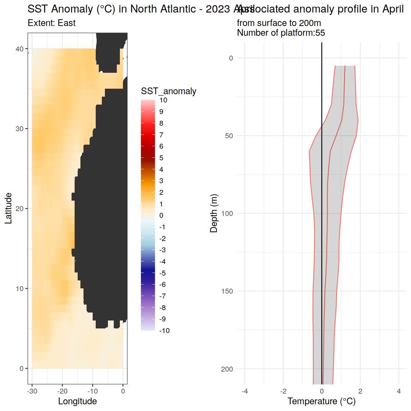

Version	Author	Date
ee73ee9	mlarriere	2024-05-12

TableGrob (1 x 2) "arrange": 2 grobs
  z     cells    name           grob
1 1 (1-1,1-1) arrange gtable[layout]
2 2 (1-1,2-2) arrange gtable[layout]

Version	Author	Date
ee73ee9	mlarriere	2024-05-12

TableGrob (1 x 2) "arrange": 2 grobs
  z     cells    name           grob
1 1 (1-1,1-1) arrange gtable[layout]
2 2 (1-1,2-2) arrange gtable[layout]

Version	Author	Date
ee73ee9	mlarriere	2024-05-12

TableGrob (1 x 2) "arrange": 2 grobs
  z     cells    name           grob
1 1 (1-1,1-1) arrange gtable[layout]
2 2 (1-1,2-2) arrange gtable[layout]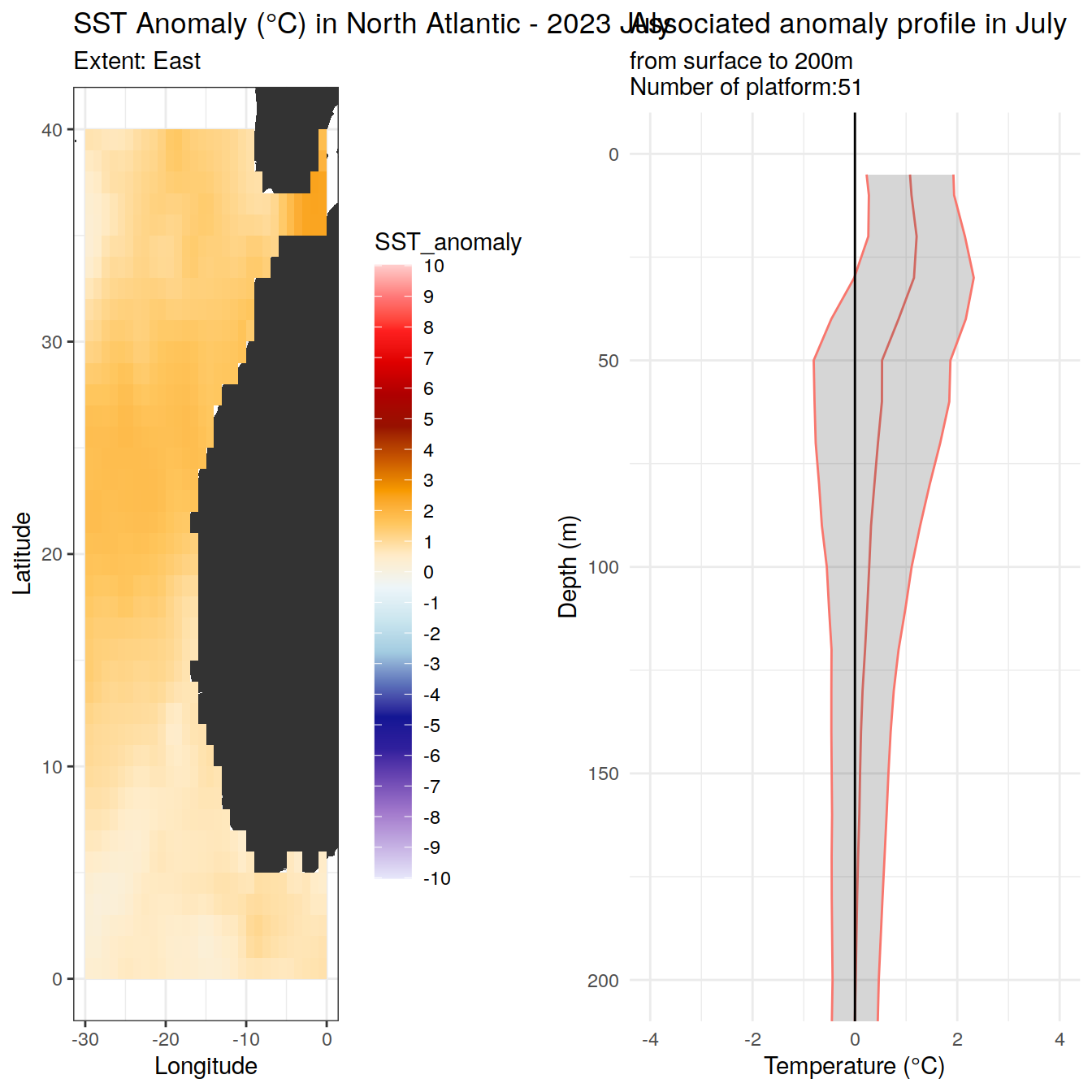

Version	Author	Date
ee73ee9	mlarriere	2024-05-12

TableGrob (1 x 2) "arrange": 2 grobs
  z     cells    name           grob
1 1 (1-1,1-1) arrange gtable[layout]
2 2 (1-1,2-2) arrange gtable[layout]

Version	Author	Date
ee73ee9	mlarriere	2024-05-12

TableGrob (1 x 2) "arrange": 2 grobs
  z     cells    name           grob
1 1 (1-1,1-1) arrange gtable[layout]
2 2 (1-1,2-2) arrange gtable[layout]

Version	Author	Date
ee73ee9	mlarriere	2024-05-12

TableGrob (1 x 2) "arrange": 2 grobs
  z     cells    name           grob
1 1 (1-1,1-1) arrange gtable[layout]
2 2 (1-1,2-2) arrange gtable[layout]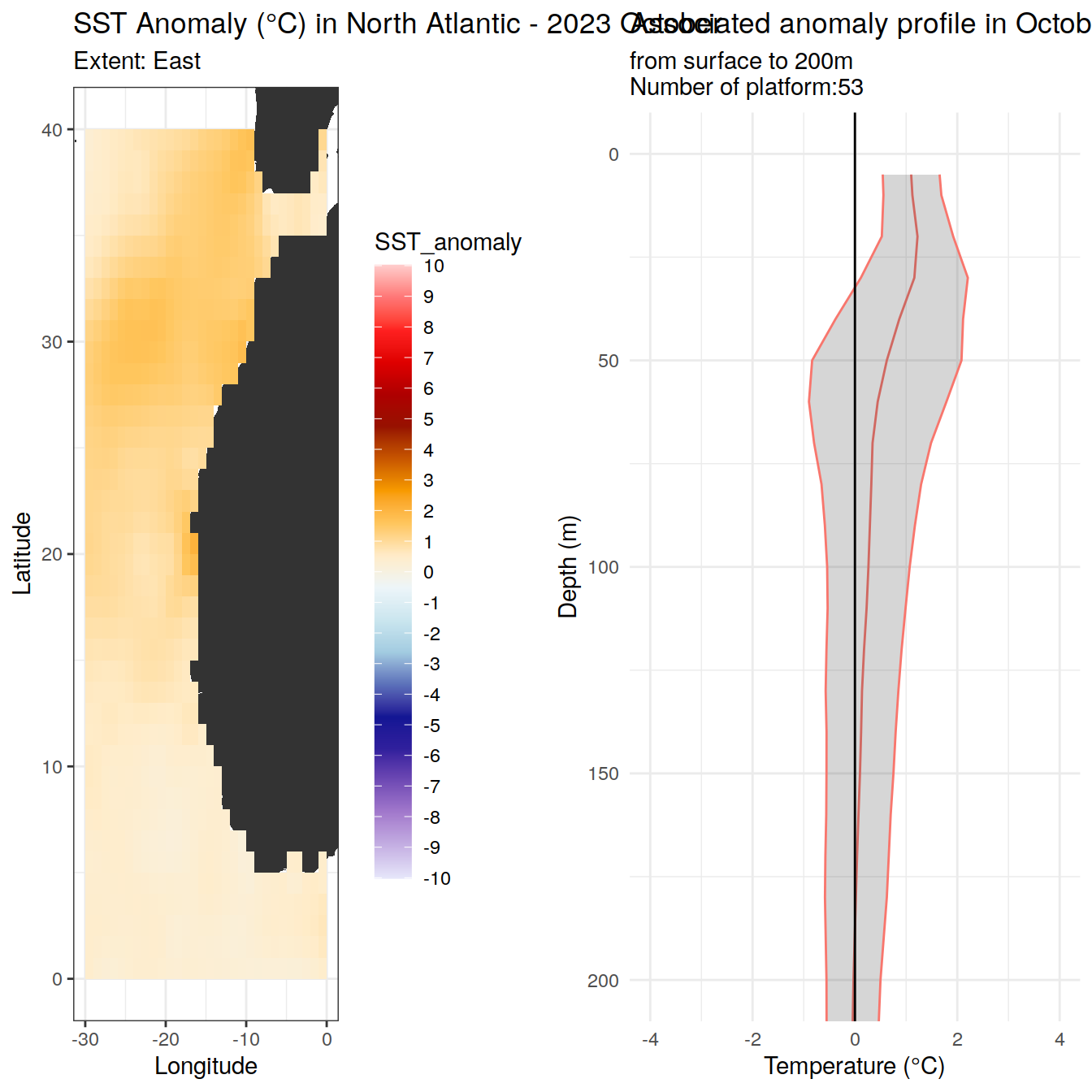

Version	Author	Date
ee73ee9	mlarriere	2024-05-12

TableGrob (1 x 2) "arrange": 2 grobs
  z     cells    name           grob
1 1 (1-1,1-1) arrange gtable[layout]
2 2 (1-1,2-2) arrange gtable[layout]

Version	Author	Date
ee73ee9	mlarriere	2024-05-12

TableGrob (1 x 2) "arrange": 2 grobs
  z     cells    name           grob
1 1 (1-1,1-1) arrange gtable[layout]
2 2 (1-1,2-2) arrange gtable[layout]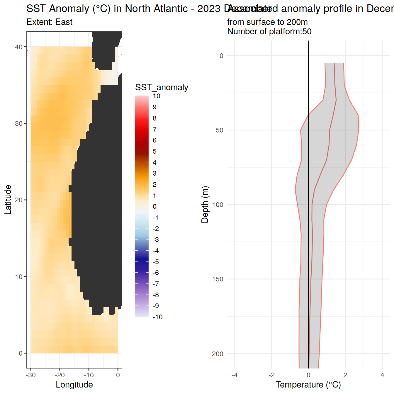

Version	Author	Date
ee73ee9	mlarriere	2024-05-12

TableGrob (1 x 2) "arrange": 2 grobs
  z     cells    name           grob
1 1 (1-1,1-1) arrange gtable[layout]
2 2 (1-1,2-2) arrange gtable[layout]

platform_counts <- aggregate(platform_number ~ month, data = heatwaves_data_east, FUN = function(x) length(unique(x)))
cycle_count_per_platform_month <- heatwaves_data_east %>%
  group_by(month, platform_number) %>%
  summarise(cycle_count = n_distinct(cycle_number))

# Tiles for SST anomaly
map_anomaly_east <- 
  east_base_map + 
  geom_tile(data=east_sst_anomaly, aes(x = lon, y = lat, fill = SST_anomaly)) +
  scale_fill_gradientn(colors = continuous_palette, limits = scale_limits, breaks = scale_breaks) +
  labs(fill = "SST Anomaly") +
  theme_minimal()

custom_labeller <- function(variable, value) {
  month_count <- platform_counts[platform_counts$month == value, "platform_number"]
  return(paste("Month:", value, "\nnumber of floats:", month_count))
}

platform_positions <- map_anomaly_east +
  geom_point(data = heatwaves_data_east, aes(x = lon, y = lat), color = "dodgerblue3") +
  labs(title = "Platform Locations") +  
  facet_wrap(~month, ncol = 3, labeller = custom_labeller)

platform_positions

Version	Author	Date
ee73ee9	mlarriere	2024-05-12

MHWs category

#Data from: https://github.com/jens-daniel-mueller/heatwave_co2_flux_2023/blob/master/analysis/mhw_stats.Rmd
#Read data
mhw_raw_2023<-read.csv(paste0(path_mhw, '/2023_mhw_raw.csv')) %>% 
  as_tibble() %>% 
  mutate(lon = ifelse(lon > 180, lon - 360, lon)) #longitudes between -180 and 180° 

#Select North Atlantic and add month attribute
mhw_raw_2023_north_atlantic<-mhw_raw_2023 %>% 
    filter(lat > 0, lon <30, lon >-100)
mhw_raw_2023_north_atlantic$month <- format(as.Date(mhw_raw_2023_north_atlantic$time), "%m")

Upscaling Surface Marine Heat Waves

#Aggregate the dataset into 1°x1° grid
argo_grid<-sst_natlantic_2023 %>% 
  ungroup() %>% 
  select(lat, lon)
  
mhw_1x1_natlantic_2023 <- mhw_raw_2023_north_atlantic %>% #----------->long process (few min)
  mutate(lat_upscale = floor(lat) + 0.5, #rounding to the lower nearest value and add an offset of 0.5 to match with Argo data grid
         lon_upscale = floor(lon) + 0.5,
         row_id = row_number() #row identifier - to facilitate comparison with original dataset
         ) %>%  
  group_by(lat = lat_upscale, #group the data by lon, lat and time
           lon = lon_upscale, 
           time) %>% 
 summarise(avg_intensity = mean(intensity),  # average intensity
           most_freq_category = names(sort(table(category), decreasing = TRUE))[1],  #Most frequent category
           row_id = first(row_id)
           ) %>%
  ungroup() %>% 
  arrange(row_id)

test<- mhw_raw_2023_north_atlantic %>% filter(time=="2023-01-01", lat<1, lat>0, lon<1, lon>0)
print(mean(test$intensity))
test1<- mhw_1x1_natlantic_2023 %>% filter(time=="2023-01-01", lat<1, lat>0, lon<1, lon>0)
print(test1)

#Adding biomes value to the surface MHWs
mhw_1x1_natlantic_2023_biomes<-left_join(mhw_1x1_natlantic_2023, biomes_subset, by=c("lat", "lon")) %>% 
  filter(!is.na(biome_value)) 

mhw_1x1_natlantic_2023_biomes$month <- format( as.Date(mhw_1x1_natlantic_2023_biomes$time), "%m")#adding month attribute

#Write upscaled MHWs dataset (1°x1°)
mhw_1x1_natlantic_2023_biomes %>% write_rds(file = paste0(path_argo_core_preprocessed,"/", "2023_surface_mhws_1x1.rds"))

Surface intensity maps

#Read upscale data
mhw_1x1_natlantic_2023_biomes <- read_rds(file = paste0(path_argo_core_preprocessed,"/", "2023_surface_mhws_1x1.rds"))

# original_plot <- base_map +
#   geom_point(data=mhw_raw_2023_north_atlantic, aes(x = lon, y = lat, color = intensity), size=0.1) +
#   scale_color_gradient(low = "blue", high = "red") +
#   labs(title = "MHW intensity - Original Data") +
#   theme_minimal()
# print(original_plot)

mhw_biomes_plot <- base_map +
  geom_point(data= mhw_1x1_natlantic_2023_biomes, aes(x = lon, y = lat, color = avg_intensity)) +
  scale_color_gradient(low = "blue", high = "red") +
  labs(title = "MHW intensity - Upscaled Data") +
  theme_minimal()
print(mhw_biomes_plot)

Surface category maps per season

mhw_season_plot_comparison<-function(original_dataset, upscale_dataset, season_of_interest, name_season){
  
  #Select data in season_of_interest
  season_original<-original_dataset %>% 
  filter(month %in% season_of_interest)
  
  season_1x1<-upscale_dataset %>% 
  filter(month %in% season_of_interest)
  
  #Plot
  plot_original<- base_map + 
  geom_point(data = season_original, aes(x = lon, y = lat, color = factor(category))) +
  scale_color_manual(values = c("I Moderate" = "darkgoldenrod1", 
                                "II Strong" = "darkorange",
                                "III Severe" = "darkred",
                                "IV Extreme" = "#21152B"), name = "Category")+
  guides(color = guide_legend(override.aes = list(shape = 15, size = 10)))+
  labs(title = paste0("Surface MHWs in ", name_season, " 2023 - resolution 0.25°x0.25°")) 
  
  plot_upscale<- base_map + 
  geom_point(data = season_1x1, aes(x = lon, y = lat, color = factor(most_freq_category)), size = 0.3) +
  scale_color_manual(values = c("I Moderate" = "darkgoldenrod1", 
                                "II Strong" = "darkorange",
                                "III Severe" = "darkred",
                                "IV Extreme" = "#21152B"), name = "Category")+
  guides(color = guide_legend(override.aes = list(shape = 15, size = 10)))+
  labs(title = paste0("Surface MHWs in ", name_season, " 2023 - resolution 1°x1°"))


  combined_plot <- grid.arrange(plot_original, plot_upscale, ncol = 2)
  print(combined_plot)
}

mhw_season_plot_comparison(mhw_raw_2023_north_atlantic, mhw_1x1_natlantic_2023_biomes, c("03", "04", "05"), "spring")
mhw_season_plot_comparison(mhw_raw_2023_north_atlantic, mhw_1x1_natlantic_2023_biomes, c("06", "07", "08"), "summer")
mhw_season_plot_comparison(mhw_raw_2023_north_atlantic, mhw_1x1_natlantic_2023_biomes, c("09", "10", "11", "12"), "autumn")
mhw_season_plot_comparison(mhw_raw_2023_north_atlantic, mhw_1x1_natlantic_2023_biomes, c("01", "02"), "winter")

mhw_season_plot<-function(upscale_dataset, months){
  months<-unique(format(as.Date(upscale_dataset$time), "%m"))
  print(months)
  #Plot
  plot_upscale<- base_map + 
  geom_point(data = upscale_dataset, aes(x = lon, y = lat, color = factor(most_freq_category)), size = 0.3) +
  scale_color_manual(values = c("I Moderate" = "darkgoldenrod1", 
                                "II Strong" = "darkorange",
                                "III Severe" = "darkred",
                                "IV Extreme" = "#21152B"), name = "Category")+
  guides(color = guide_legend(override.aes = list(shape = 15, size = 10)))+
  labs(title = paste0("Surface MHWs in 2023"),
       subtitle = paste0("Months: ", paste(months, collapse = ", ") ,"\nresolution 1°x1°"))
  return(plot_upscale)
}

#Select data in season_of_interest
spring_1x1<-mhw_1x1_natlantic_2023_biomes %>% 
  filter(month %in% c("03", "04", "05"))
summer_1x1<-mhw_1x1_natlantic_2023_biomes %>% 
  filter(month %in% c("06", "07", "08"))
autumn_1x1<-mhw_1x1_natlantic_2023_biomes %>% 
  filter(month %in% c("09", "10", "11", "12"))
winter_1x1<-mhw_1x1_natlantic_2023_biomes %>% 
  filter(month %in% c("01", "02"))

#Plot MHWs
spring_plot_1x1<-mhw_season_plot(spring_1x1, "spring")
summer_plot_1x1<-mhw_season_plot(summer_1x1, "summer")
autumn_plot_1x1<-mhw_season_plot(autumn_1x1, "autumn")
winter_plot_1x1<-mhw_season_plot(winter_1x1, "winter")

combined_plot <- grid.arrange(winter_plot_1x1, spring_plot_1x1, summer_plot_1x1, autumn_plot_1x1, ncol = 2, nrow=2)
print(combined_plot)

Strong MHWs regions

#Time in the same format in the 2 dataframes
argo_data_2023 <- sst_with_platform_2023 %>%
  mutate(time = as.Date(date))
mhw_1x1_natlantic_2023_biomes <- mhw_1x1_natlantic_2023_biomes %>%
  mutate(time = as.Date(time))

#Associating mhws category to the argo profiles
argo_mhws_categ<-left_join(mhw_1x1_natlantic_2023_biomes, argo_data_2023, by=c("lat", "lon", "time")) %>% 
  filter(!is.na(platform_number)) %>%  #select only locations where there is an argo float
  rename(biome_value=biome_value.x) %>% 
  select(platform_number,cycle_number,
         depth, lat, lon, time, 
         avg_intensity, most_freq_category, 
         biome_value, temp) #Cleaning dataset

#Adding temperature anomaly
argo_anomaly_2023 <- argo_anomaly_2023 %>%
  mutate(time = as.Date(date)) 

#Datasets for each surface MHWs category
mhws_surface_categorisation<- function(argo_categ_dataset, anomaly_dataset, category){
  argo_surf_cat<-filter(argo_categ_dataset, most_freq_category==category)
  argo_anomaly_cat<- left_join(anomaly_dataset, argo_surf_cat, 
                               by=c("platform_number", "cycle_number","lat", "lon", "depth", "time", "biome_value")) %>% 
  filter(!is.na(anomaly), !is.na(most_freq_category))
  
  return(argo_anomaly_cat)
}

argo_anomaly_moderate<- mhws_surface_categorisation(argo_mhws_categ, argo_anomaly_2023, category='I Moderate')
argo_anomaly_strong<- mhws_surface_categorisation(argo_mhws_categ, argo_anomaly_2023, category='II Strong')
argo_anomaly_severe<- mhws_surface_categorisation(argo_mhws_categ, argo_anomaly_2023, category='III Severe')
argo_anomaly_extreme<- mhws_surface_categorisation(argo_mhws_categ, argo_anomaly_2023, category='IV Extreme')

final_mhw_argo_cat<-bind_rows(argo_anomaly_moderate,
                              argo_anomaly_strong,
                              argo_anomaly_severe,
                              argo_anomaly_extreme)

Mean anomaly temperature profile

Per biomes and months

We investigate the mean temperature anomaly profile for each biome and over months in 2023.

plot_anomaly_profiles_biomes <- function(data, biome_chosen) {
  
  # Filter data for the chosen biome
  biome_data <- filter(data, biome_value == biome_chosen)
  
  # Anomaly statistics
  anomaly_overall_mean <- biome_data %>%
    group_by(depth, month, biome_value) %>% 
    summarise(temp_count = n(),
              temp_anomaly_mean = mean(anomaly, na.rm = TRUE),
              temp_anomaly_sd = sd(anomaly, na.rm = TRUE))
  
  # Subtitle and color based on biome chosen
  subtitle <- switch(biome_chosen,
                     "1" = "SPSS",
                     "2" = "STSS",
                     "3" = "STPS")
  
  color_SPSS <- "darkblue"
  color_STSS <- "darkorange"
  color_STPS <- "darkred"
  
  colors <- c("1" = color_SPSS, "2" = color_STSS, "3" = color_STPS)
  
  # Anomaly plot
  ggplot(anomaly_overall_mean) +
    geom_path(aes(x = temp_anomaly_mean, y = depth, color = factor(month))) +
    geom_ribbon(aes(xmax = temp_anomaly_mean + temp_anomaly_sd,
                    xmin = temp_anomaly_mean - temp_anomaly_sd,
                    y = depth, fill = factor(biome_value)), alpha = 0.4) +
    geom_vline(xintercept = 0) +
    scale_y_reverse() +
    coord_cartesian(xlim =  c(-4.5, 6)) +
    scale_x_continuous(breaks = c(-4, -2, 0, 2, 4, 6)) +
    labs(title = paste0('Mean Temperature anomaly profiles - up to 600m depth'),
         x = "Temperature anomaly (°C)", y = 'depth (m)', color = "Biome") +
    scale_color_manual(values = colors[biome_chosen],  
                       labels = subtitle) +
    scale_fill_manual(values = colors[biome_chosen], 
                      name = "Biome",  labels = subtitle) +
    facet_wrap(~ month, ncol = 3, labeller = labeller(month.abb)) +
    theme(axis.text.x = element_text(angle = 0, hjust = 1)) +
    theme(legend.position = "bottom")
  
}

plot_anomaly_profiles_biomes(final_mhw_argo_cat, 1)
plot_anomaly_profiles_biomes(final_mhw_argo_cat, 2)
plot_anomaly_profiles_biomes(final_mhw_argo_cat, 3)

Floats classification

We classify marine heat waves according to their intensity and propagation over the water column:

When the temperature anomaly is equal to or greater than 1°C, we consider the anomaly to be big, otherwise it is considered as small.

Then we look at the vertical propagation of the MHWS: - Shallow MHWs: When a big anomaly is detected between 0 and 100 meters depth.

- Medium MHWs: When a big anomaly is detected between 0 and 200 meters depth.

- Deep MHWs: When a big anomaly is detected between 0 and 600 meters depth.

# Defining the anomaly class as a function of anomaly value and depth
threshold <- argo_anomaly_moderate %>%
  filter(anomaly >= 1) %>% # Look only at positive anomaly values 
    group_by(depth) %>%
    summarise(depth_threshold = max(depth))
  
argo_anomaly_dataset <- argo_anomaly_moderate %>%
  mutate(anomaly_class = ifelse(anomaly >= 1 & depth <= threshold$depth_threshold, "Big", "Small")) %>%
  mutate(anomaly_class = factor(anomaly_class, levels = c("Big", "Small")))

# Group the data by float identifiers
max_depth_by_float <- argo_anomaly_moderate %>%
  filter(anomaly >= 1) %>%
  group_by(file_id, lat, lon) %>%
  summarise(max_depth = max(depth))

# Define mhw_class based on the maximum depth
max_depth_by_float <- max_depth_by_float %>%
  mutate(mhw_class = case_when(
    max_depth <= 100 ~ "Shallow",
    max_depth <= 200 ~ "Medium",
    TRUE ~ "Deep"
  ))

#Combining datasets
final_mhw_argo_cat<-left_join(max_depth_by_float, argo_anomaly_dataset, by=c("file_id", "lat","lon") )

 
plot_anomaly_categorisation <- function(anomaly_data) {
  anomaly_classes <- anomaly_data %>%
    distinct(depth, anomaly_class)

    ggplot(anomaly_data) +
    geom_rect(data = anomaly_data %>% distinct(depth, anomaly_class),
              aes(xmin = -Inf, xmax = Inf, ymin = lag(depth), ymax = depth, fill = anomaly_class),
              inherit.aes = FALSE) +
    geom_path(aes(x = anomaly , y = depth)) +
    geom_vline(xintercept = 0) +
    scale_fill_manual(values = c("Big" = "lightblue", "Small" = "lightyellow"), 
                                            name = "Anomaly Class",  labels = c("Big Anomaly", "Small Anomaly")
) +
    scale_y_reverse() +
    coord_cartesian(xlim = c(-4.5, 6)) +
    scale_x_continuous(breaks = c(-4, -2, 0, 2, 4, 6)) +
    labs(title = paste0('Anomaly profile in ', month.name[unique(month(anomaly_data$time))], ' 2023'),
         subtitle = paste0('Location: (', unique(anomaly_data$lat), ',', unique(anomaly_data$lon),')\n',
                          'Type of surface MHW: ', unique(anomaly_data$most_freq_category),"\n",
                           'Type of argo MHW: ', unique(anomaly_data$mhw_class)),
         x = "Temperature anomaly (°C)", y = 'depth (m)')
}

shallow<-plot_anomaly_categorisation(final_mhw_argo_cat %>% filter(file_id==20))
medium<-plot_anomaly_categorisation(final_mhw_argo_cat %>% filter(file_id==10))
deep<-plot_anomaly_categorisation(final_mhw_argo_cat %>% filter(file_id==6396))

combined_plot <- grid.arrange(shallow, medium, deep, ncol = 3)
print(combined_plot)

sessionInfo()

R version 4.2.2 (2022-10-31)
Platform: x86_64-pc-linux-gnu (64-bit)
Running under: openSUSE Leap 15.5

Matrix products: default
BLAS:   /usr/local/R-4.2.2/lib64/R/lib/libRblas.so
LAPACK: /usr/local/R-4.2.2/lib64/R/lib/libRlapack.so

locale:
 [1] LC_CTYPE=en_US.UTF-8       LC_NUMERIC=C              
 [3] LC_TIME=en_US.UTF-8        LC_COLLATE=en_US.UTF-8    
 [5] LC_MONETARY=en_US.UTF-8    LC_MESSAGES=en_US.UTF-8   
 [7] LC_PAPER=en_US.UTF-8       LC_NAME=C                 
 [9] LC_ADDRESS=C               LC_TELEPHONE=C            
[11] LC_MEASUREMENT=en_US.UTF-8 LC_IDENTIFICATION=C       

attached base packages:
[1] stats     graphics  grDevices utils     datasets  methods   base     

other attached packages:
 [1] broom_1.0.5          paletteer_1.6.0      cluster_2.1.6       
 [4] gridExtra_2.3        scatterplot3d_0.3-44 viridis_0.6.2       
 [7] viridisLite_0.4.1    ggOceanMaps_1.3.4    ggspatial_1.1.7     
[10] oce_1.7-10           gsw_1.1-1            lubridate_1.9.0     
[13] timechange_0.1.1     forcats_0.5.2        stringr_1.5.0       
[16] dplyr_1.1.3          purrr_1.0.2          readr_2.1.3         
[19] tidyr_1.3.0          tibble_3.2.1         ggplot2_3.4.4       
[22] tidyverse_1.3.2      workflowr_1.7.0     

loaded via a namespace (and not attached):
 [1] googledrive_2.0.0   colorspace_2.0-3    ellipsis_0.3.2     
 [4] class_7.3-20        rprojroot_2.0.3     fs_1.5.2           
 [7] rstudioapi_0.15.0   proxy_0.4-27        farver_2.1.1       
[10] fansi_1.0.3         xml2_1.3.3          codetools_0.2-18   
[13] cachem_1.0.6        knitr_1.41          jsonlite_1.8.3     
[16] dbplyr_2.2.1        rgeos_0.5-9         compiler_4.2.2     
[19] httr_1.4.4          backports_1.4.1     assertthat_0.2.1   
[22] fastmap_1.1.0       gargle_1.2.1        cli_3.6.1          
[25] later_1.3.0         htmltools_0.5.8.1   tools_4.2.2        
[28] gtable_0.3.1        glue_1.6.2          maps_3.4.1         
[31] Rcpp_1.0.10         cellranger_1.1.0    jquerylib_0.1.4    
[34] RNetCDF_2.6-1       raster_3.6-11       vctrs_0.6.4        
[37] lwgeom_0.2-10       xfun_0.35           ps_1.7.2           
[40] rvest_1.0.3         lifecycle_1.0.3     ncmeta_0.3.5       
[43] googlesheets4_1.0.1 terra_1.7-65        getPass_0.2-2      
[46] scales_1.2.1        hms_1.1.2           promises_1.2.0.1   
[49] parallel_4.2.2      rematch2_2.1.2      yaml_2.3.6         
[52] sass_0.4.4          stringi_1.7.8       highr_0.9          
[55] e1071_1.7-12        rlang_1.1.1         pkgconfig_2.0.3    
[58] evaluate_0.18       lattice_0.20-45     sf_1.0-9           
[61] labeling_0.4.2      processx_3.8.0      tidyselect_1.2.0   
[64] magrittr_2.0.3      R6_2.5.1            generics_0.1.3     
[67] DBI_1.2.2           pillar_1.9.0        haven_2.5.1        
[70] whisker_0.4         withr_2.5.0         units_0.8-0        
[73] stars_0.6-0         abind_1.4-5         sp_1.5-1           
[76] modelr_0.1.10       crayon_1.5.2        KernSmooth_2.23-20 
[79] utf8_1.2.2          tzdb_0.3.0          rmarkdown_2.18     
[82] grid_4.2.2          readxl_1.4.1        callr_3.7.3        
[85] git2r_0.30.1        reprex_2.0.2        digest_0.6.30      
[88] classInt_0.4-8      httpuv_1.6.6        munsell_0.5.0      
[91] bslib_0.4.1

Marine Heat Waves categorisation

Marguerite Larriere & Jens Daniel Müller

12 May, 2024