OceanSODA-Argo pH
Pasqualina Vonlanthen, David Stappard & Jens Daniel Müller
13 May, 2024
Last updated: 2024-05-13
Checks: 7 0
Knit directory:
bgc_argo_r_argodata/analysis/
This reproducible R Markdown analysis was created with workflowr (version 1.7.0). The Checks tab describes the reproducibility checks that were applied when the results were created. The Past versions tab lists the development history.
Great! Since the R Markdown file has been committed to the Git repository, you know the exact version of the code that produced these results.
Great job! The global environment was empty. Objects defined in the global environment can affect the analysis in your R Markdown file in unknown ways. For reproduciblity it’s best to always run the code in an empty environment.
The command set.seed(20211008) was run prior to running
the code in the R Markdown file. Setting a seed ensures that any results
that rely on randomness, e.g. subsampling or permutations, are
reproducible.
Great job! Recording the operating system, R version, and package versions is critical for reproducibility.
Nice! There were no cached chunks for this analysis, so you can be confident that you successfully produced the results during this run.
Great job! Using relative paths to the files within your workflowr project makes it easier to run your code on other machines.
Great! You are using Git for version control. Tracking code development and connecting the code version to the results is critical for reproducibility.
The results in this page were generated with repository version 91e6028. See the Past versions tab to see a history of the changes made to the R Markdown and HTML files.
Note that you need to be careful to ensure that all relevant files for
the analysis have been committed to Git prior to generating the results
(you can use wflow_publish or
wflow_git_commit). workflowr only checks the R Markdown
file, but you know if there are other scripts or data files that it
depends on. Below is the status of the Git repository when the results
were generated:
Ignored files:
    Ignored:    .Rproj.user/

Untracked files:
    Untracked:  analysis/draft.Rmd
    Untracked:  load_argo_core_output.txt

Unstaged changes:
    Deleted:    analysis/MHWs_categorisation.Rmd
    Modified:   analysis/_site.yml
    Modified:   analysis/child/cluster_analysis_base.Rmd
    Modified:   analysis/coverage_maps_North_Atlantic.Rmd
    Modified:   analysis/load_broullon_DIC_TA_clim.Rmd
    Modified:   code/Workflowr_project_managment.R
    Modified:   code/start_background_job.R
    Modified:   code/start_background_job_load.R
    Modified:   code/start_background_job_partial.R
Note that any generated files, e.g. HTML, png, CSS, etc., are not included in this status report because it is ok for generated content to have uncommitted changes.
These are the previous versions of the repository in which changes were
made to the R Markdown (analysis/oceanSODA_argo_pH.Rmd) and
HTML (docs/oceanSODA_argo_pH.html) files. If you’ve
configured a remote Git repository (see ?wflow_git_remote),
click on the hyperlinks in the table below to view the files as they
were in that past version.
| File | Version | Author | Date | Message |
|---|---|---|---|---|
| html | af6594f | mlarriere | 2024-05-13 | Build site. |
| html | af44bcd | mlarriere | 2024-04-26 | Build site. |
| html | 780276c | mlarriere | 2024-04-19 | Build site. |
| html | 1a72545 | mlarriere | 2024-04-12 | Build site. |
| html | c076fba | mlarriere | 2024-04-12 | Build site. |
| html | 91f08a6 | mlarriere | 2024-04-07 | Build site. |
| html | db21f55 | mlarriere | 2024-04-06 | Build site. |
| html | de83e45 | mlarriere | 2024-04-01 | Build site. |
| html | f9de50e | ds2n19 | 2024-01-01 | Build site. |
| html | 07d4eb8 | ds2n19 | 2023-12-20 | Build site. |
| html | fa6cf38 | ds2n19 | 2023-12-14 | Build site. |
| Rmd | 64fd104 | ds2n19 | 2023-12-14 | revised coverage analysis and SO focused cluster analysis. |
| html | f110b74 | ds2n19 | 2023-12-13 | Build site. |
| Rmd | fa9795c | ds2n19 | 2023-12-12 | dependencies listed are start of markdown files. |
| html | e60ebd2 | ds2n19 | 2023-12-07 | Build site. |
| html | cec2a2a | ds2n19 | 2023-11-24 | Build site. |
| Rmd | 59f5cc4 | ds2n19 | 2023-11-23 | Moved spatiotemporal analysis to use aligned profiles. |
| html | 80c16c2 | ds2n19 | 2023-11-15 | Build site. |
| html | 4b55c43 | ds2n19 | 2023-10-12 | Build site. |
| html | 1ae81b3 | ds2n19 | 2023-10-11 | reworked core load process to work initially by year and then finally create consolidated all years files. |
| html | 44f5720 | ds2n19 | 2023-10-09 | manual commit |
| Rmd | ce19a66 | ds2n19 | 2023-10-04 | Revised version of OceanSODA product -v2023 |
| html | 7b3d8c5 | pasqualina-vonlanthendinenna | 2022-08-29 | Build site. |
| html | bdd516d | pasqualina-vonlanthendinenna | 2022-05-23 | Build site. |
| html | 4173c20 | jens-daniel-mueller | 2022-05-12 | Build site. |
| html | dfe89d7 | jens-daniel-mueller | 2022-05-12 | Build site. |
| html | 710edd4 | jens-daniel-mueller | 2022-05-11 | Build site. |
| Rmd | 2f20a76 | jens-daniel-mueller | 2022-05-11 | rebuild all after subsetting AB profiles and code cleaning |
Task
Compare BGC-Argo pH data to pH from the OceanSODA surface data product
Dependencies
OceanSODA.rds - bgc preprocessed folder, created by load_OceanSODA.
pH_bgc_observed.rds - bgc preprocessed folder, created by ph_align_climatology. Not this file is written BEFORE the vertical alignment stage.
Outputs
argo_OceanSODA.rds - bgc preprocessed folder
theme_set(theme_bw())Load data
Load in surface Argo pH and the OceanSODA pH, gridded to 1x1º
path_argo <- '/nfs/kryo/work/updata/bgc_argo_r_argodata'
path_argo_preprocessed <- paste0(path_argo, "/preprocessed_bgc_data")
path_emlr_utilities <- "/nfs/kryo/work/jenmueller/emlr_cant/utilities/files/"

path_argo <- '/nfs/kryo/work/datasets/ungridded/3d/ocean/floats/bgc_argo'
# /nfs/kryo/work/datasets/ungridded/3d/ocean/floats/bgc_argo/preprocessed_bgc_data
path_argo_preprocessed <- paste0(path_argo, "/preprocessed_bgc_data")
# load in OceanSODA data and Argo pH
OceanSODA <- read_rds(file = paste0(path_argo_preprocessed, "/OceanSODA.rds"))
argo <- read_rds(file = paste0(path_argo_preprocessed, '/pH_bgc_observed.rds')) %>%
filter(between(depth, 0, 20))
# argo <-
# read_rds(file = paste0(path_argo_preprocessed, "/bgc_merge_flag_AB.rds")) %>%
# filter(between(depth, 0, 20)) %>%
# mutate(year = year(date),
# month = month(date)) %>%
# select(-c(
# temp_adjusted,
# temp_adjusted_qc,
# temp_adjusted_error,
# profile_temp_qc
# ))
# for plotting later, load in region and coastline information
# region_masks_all_seamask_2x2 <- read_rds(file = paste0(
# path_argo_preprocessed, "/region_masks_all_seamask_2x2.rds"))
#
# region_masks_all_2x2 <- read_rds(file = paste0(path_argo_preprocessed, "/region_masks_all_2x2.rds"))
#
# region_masks_all_1x1 <- read_rds(file = paste0(path_argo_preprocessed, "/region_masks_all_1x1.rds"))
nm_biomes <- read_rds(file = paste0(path_argo_preprocessed, "/nm_biomes.rds"))# read in the map from updata
map <-
read_rds(paste(path_emlr_utilities,
"map_landmask_WOA18.rds",
sep = ""))Harmonise the two datasets
Calculate monthly average pH for Argo pH for each lon/lat grid, centered on the 15th of each month, to match the format of OceanSODA
argo_monthly <- argo %>%
  mutate(year_month = format_ISO8601(date, precision = "ym"), .after = 'date') %>%
  group_by(year, month, year_month, date, lat, lon) %>%
  summarise(
    argo_ph_month = mean(ph_in_situ_total_adjusted, na.rm = TRUE)
  ) %>%
  ungroup() %>%
  select(
    date,
    year_month,
    year,
    month,
    lon,
    lat,
    argo_ph_month
  )
Join the two datasets
OceanSODA <- OceanSODA %>%
  mutate(year_month = format_ISO8601(date, precision = "ym")) %>%
  rename(date_OceanSODA = date)
  # change date format in OceanSODA to match argo date (yyyy-mm)

argo_OceanSODA <- left_join(argo_monthly, OceanSODA) %>%
  rename(OceanSODA_ph = ph_total,
         OceanSODA_ph_error = ph_total_uncert)
argo_OceanSODA %>%
write_rds(file = paste0(path_argo_preprocessed, "/argo_OceanSODA.rds"))Southern Ocean surface pH
The focus here is on Southern Ocean surface pH, south of 30ºS, as defined in the RECCAP biome regions
# region_masks_all_1x1_SO <- region_masks_all_1x1 %>%
#   filter(region == 'southern',
#          value != 0)

# keep only Southern Ocean data
argo_OceanSODA_SO <- inner_join(argo_OceanSODA, nm_biomes)
Monthly climatological OceanSODA pH
Map monthly mean pH from the OceanSODA data product
Climatological OceanSODA pH
# calculate average monthly pH between April 2014 and August 2021
argo_OceanSODA_SO_clim <- argo_OceanSODA_SO %>%
  group_by(lon, lat, month) %>%
  summarise(
    clim_OceanSODA_ph = mean(OceanSODA_ph, na.rm = TRUE),
    clim_argo_ph = mean(argo_ph_month, na.rm = TRUE),
    offset_clim = clim_OceanSODA_ph - clim_argo_ph
  ) %>%
  ungroup()

# regrid to a 2x2 grid for mapping
argo_OceanSODA_SO_clim_2x2 <- argo_OceanSODA_SO_clim %>%
  mutate(
    lat = cut(lat, seq(-90, 90, 2), seq(-89, 89, 2)),
    lat = as.numeric(as.character(lat)),
    lon = cut(lon, seq(20, 380, 2), seq(21, 379, 2)),
    lon = as.numeric(as.character(lon))
  ) %>%
  group_by(lon, lat, month) %>%
  summarise(
    clim_OceanSODA_ph = mean(clim_OceanSODA_ph, na.rm = TRUE),
    clim_argo_ph = mean(clim_argo_ph, na.rm = TRUE),
    offset_clim = mean(offset_clim, na.rm = TRUE)
  ) %>%
  ungroup()

map +
  geom_tile(data = argo_OceanSODA_SO_clim_2x2,
            aes(lon, lat, fill = clim_OceanSODA_ph)) +
  lims(y = c(-85, -25)) +
  scale_fill_viridis_c() +
  labs(x = 'lon',
       y = 'lat',
       fill = 'pH',
       title = 'Monthly climatological \nOceanSODA pH') +
  theme(legend.position = 'right') +
  facet_wrap(~month, ncol = 2)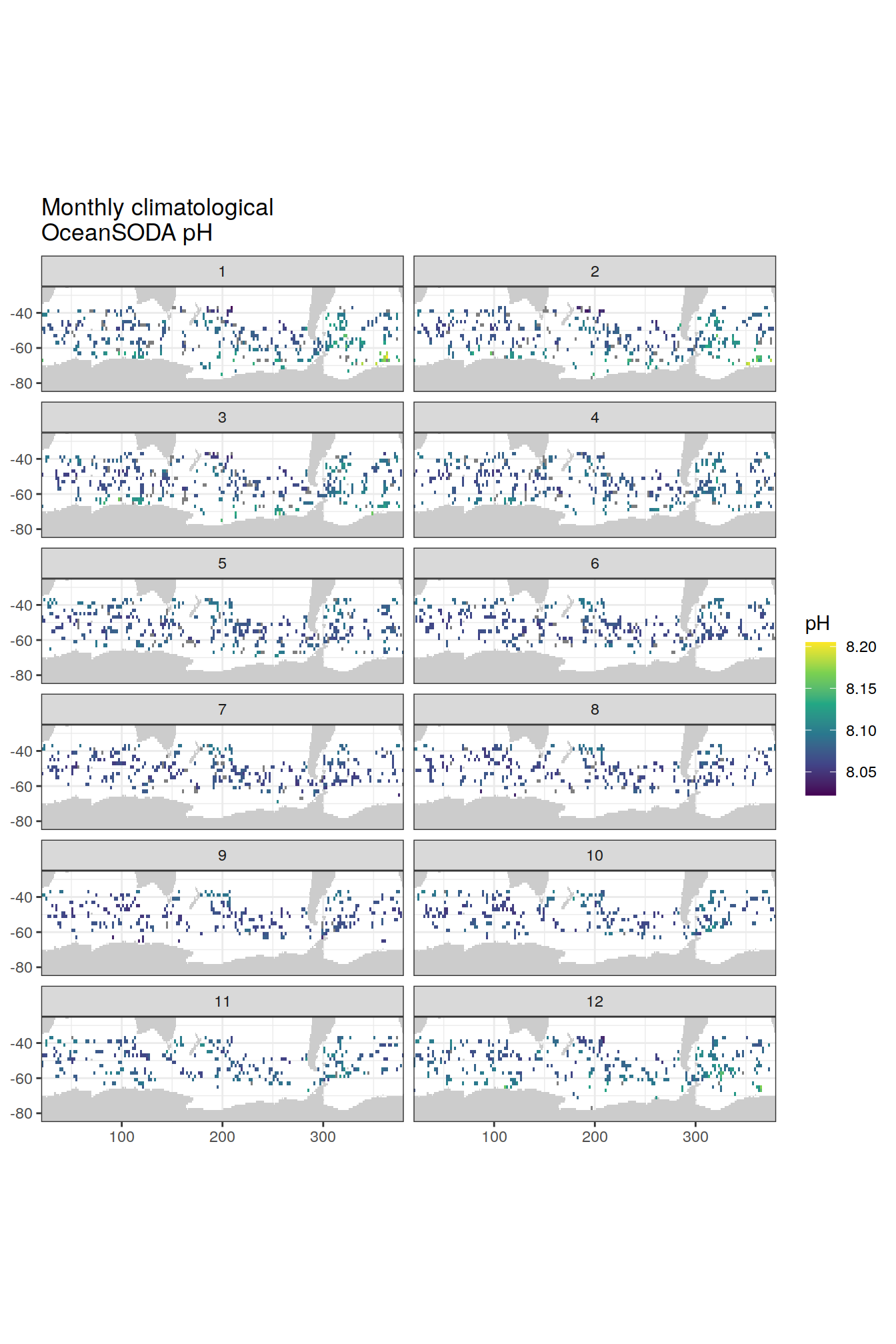
# plot the climatological monthly OceanSODA pH on a polar projection
basemap(limits = -32, data = argo_OceanSODA_SO_clim_2x2) +   # change to polar projection
  geom_spatial_tile(data = argo_OceanSODA_SO_clim_2x2,
                    aes(x = lon,
                        y = lat,
                        fill = clim_OceanSODA_ph),
                    linejoin = 'mitre',
                    col = 'transparent',
                    detail = 60)+
  scale_fill_viridis_c()+
  theme(legend.position = 'right')+
  labs(x = 'lon',
       y = 'lat',
       fill = 'pH',
       title = 'monthly climatological \nOceanSODA pH')+
  facet_wrap(~month, ncol = 2)
Climatological monthly Argo pH
Climatological Argo pH
map +
  geom_tile(data = argo_OceanSODA_SO_clim_2x2,
            aes(lon, lat, fill = clim_argo_ph)) +
  lims(y = c(-85, -25)) +
  scale_fill_viridis_c() +
  labs(x = 'lon',
       y = 'lat',
       fill = 'pH',
       title = 'Monthly climatological \nArgo pH') +
  theme(legend.position = 'right') +
  facet_wrap(~month, ncol = 2)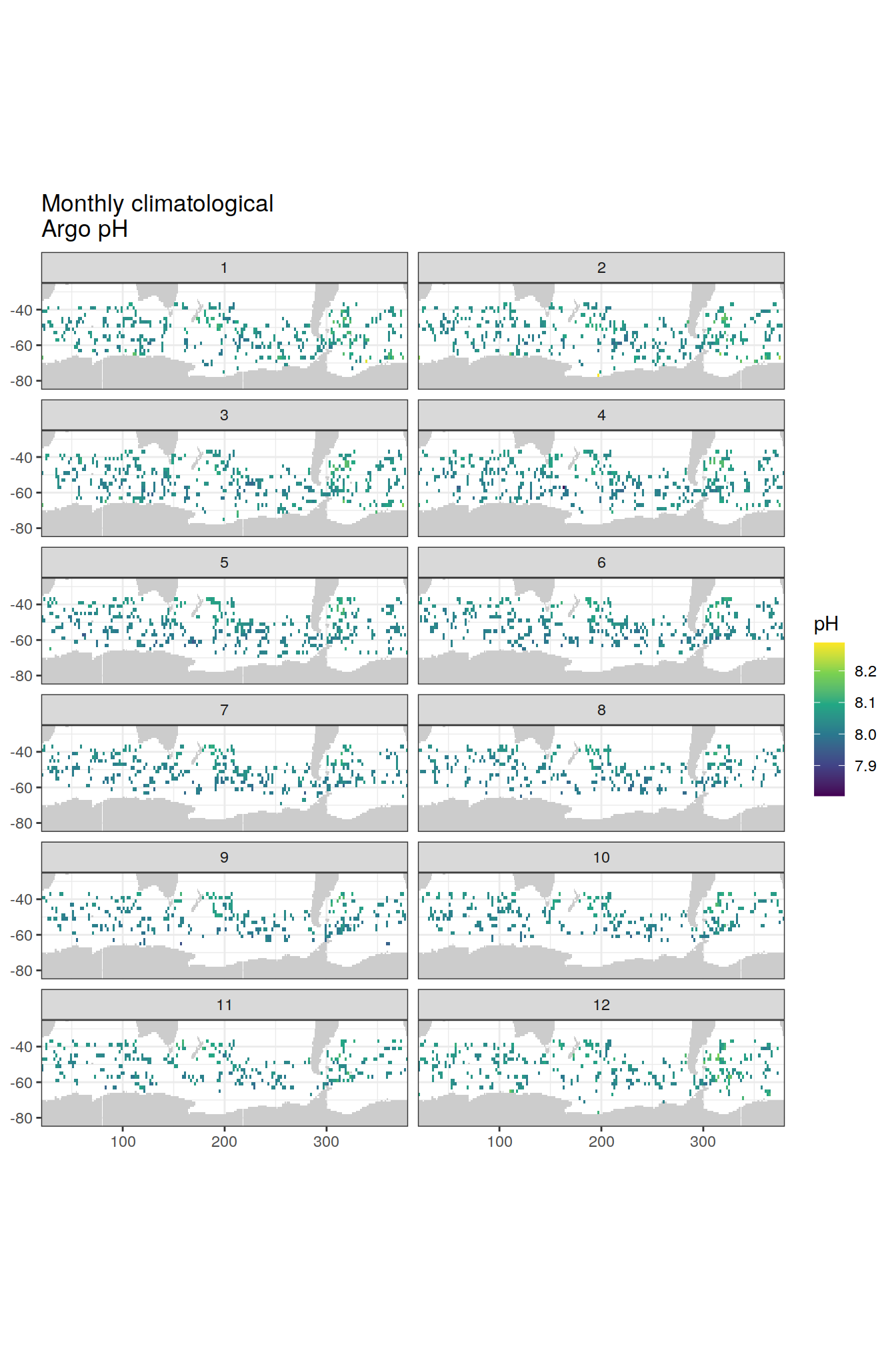
basemap(limits = -32, data = argo_OceanSODA_SO_clim_2x2) +   # change to polar projection
  geom_spatial_tile(data = argo_OceanSODA_SO_clim_2x2,
                    aes(x = lon,
                        y = lat,
                        fill = clim_argo_ph),
                    linejoin = 'mitre',
                    col = 'transparent',
                    detail = 60)+
  scale_fill_viridis_c()+
  theme(legend.position = 'right')+
  labs(x = 'lon',
       y = 'lat',
       fill = 'pH',
       title = 'monthly climatological \nArgo pH')+
  facet_wrap(~month, ncol = 2)
Timeseries of monthly OceanSODA pH
Evolution of monthly surface pH, for the three Southern Ocean RECCAP regions
map +
  geom_raster(data = nm_biomes,
              aes(x = lon,
                  y = lat,
                  fill = biome_name)) +
  labs(title = 'Southern Ocean Mayot biomes',
       fill = 'biome')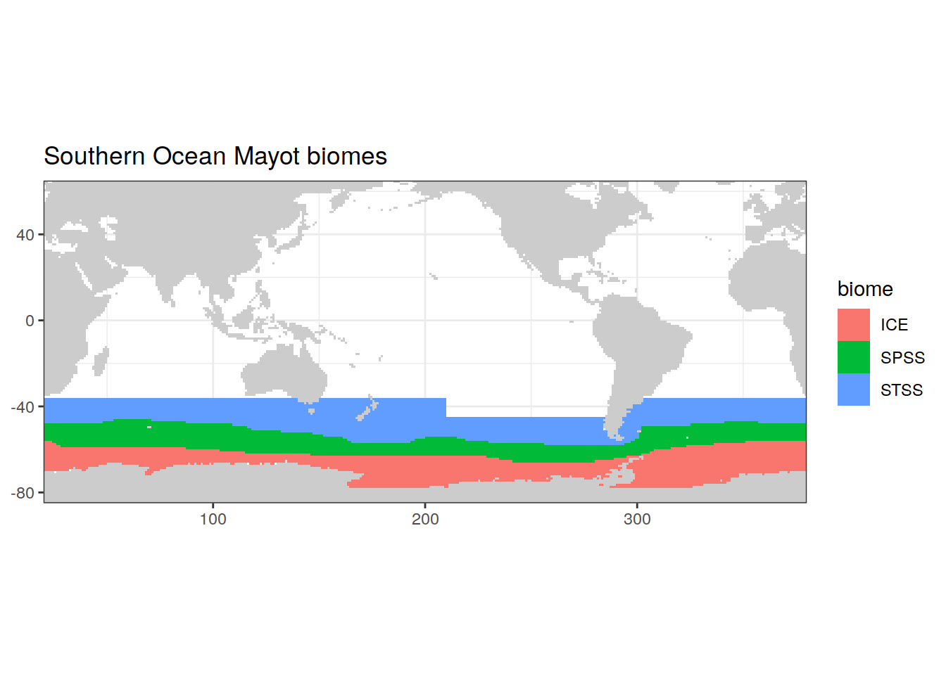
# plot timeseries of monthly OceanSODA pH
argo_OceanSODA_SO_clim_regional <- argo_OceanSODA_SO %>%
  select(year, month, biome_name, OceanSODA_ph, argo_ph_month) %>%
  pivot_longer(c(OceanSODA_ph,argo_ph_month),
               values_to = "ph",
               names_to = "data_source") %>%
  group_by(year, month, biome_name, data_source) %>%  # compute regional mean OceanSODA pH for the three biomes
  summarise(ph = mean(ph, na.rm = TRUE)) %>%
  ungroup()
argo_OceanSODA_SO_clim_regional %>%
ggplot(aes(x = year,
y = ph,
col = biome_name)) +
facet_grid(month ~ data_source) +
geom_line() +
geom_point() +
labs(x = 'year',
y = 'pH in situ (total scale)',
title = 'monthly mean pH (Southern Ocean)',
col = 'region')argo_OceanSODA_SO_clim_regional %>%
# filter(year != 2014,
# year != 2021) %>%
ggplot(aes(x = month,
y = ph,
group = year,
col = as.character(year)))+
geom_line()+
geom_point()+
scale_x_continuous(breaks = seq(1, 12, 2))+
facet_grid(biome_name~data_source)+
labs(x = 'month',
y = 'pH in situ (total scale)',
title = 'monthly mean OceanSODA pH (Southern Ocean)',
col = 'year')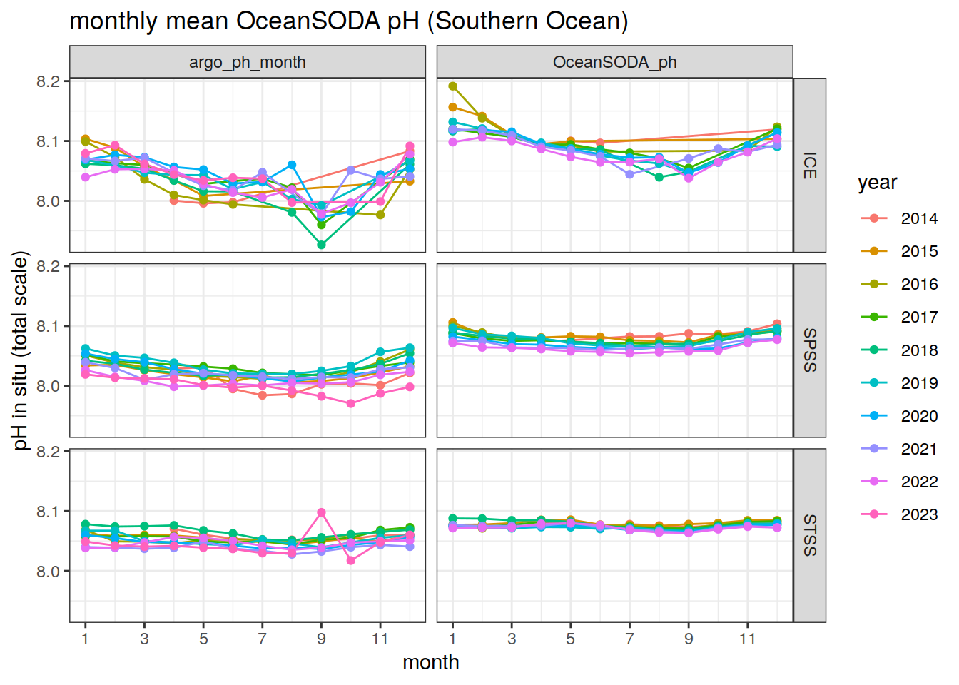
Comparison between Argo and OceanSODA pH
Calculate the difference between Argo and OceanSODA pH values
Offset between in-situ monthly pH:
argo_OceanSODA_SO <- argo_OceanSODA_SO %>%
  mutate(offset = OceanSODA_ph - argo_ph_month)

argo_OceanSODA_SO %>%
  drop_na() %>%
  ggplot() +
  geom_hline(yintercept = 0, size = 1)+
  geom_point(aes(x = year_month, y = offset, col = biome_name), size = 0.7, pch = 19) +
  scale_x_discrete(breaks = c('2014-01', '2015-01', '2016-01', '2017-01', '2018-01', '2019-01', '2020-01', '2021-01', '2022-01', '2023-01'))+
  labs(title = 'oceanSODA pH - Argo pH',
       x = 'date',
       y = 'offset (pH units)',
       col = 'region')
argo_OceanSODA_SO %>%
  drop_na() %>%
  ggplot(aes(x = OceanSODA_ph, y = argo_ph_month))+
  # geom_point(pch = 19, size = 0.7)+
  geom_bin2d(aes(x = OceanSODA_ph, y = argo_ph_month), size = 0.3, bins = 60)+
  scale_fill_viridis_c()+
  lims(x = c(7.8, 8.25),
       y = c(7.8, 8.25)) +
  geom_abline(slope = 1, intercept = 0)+
  facet_wrap(~biome_name)+
  labs(x = 'OceanSODA pH (total scale)',
       y = 'Argo pH (total scale)',
       title = 'Southern Ocean regional pH')
Mean offset between in-situ OceanSODA pH and in-situ Argo pH
mean_insitu_offset <- argo_OceanSODA_SO %>%
  group_by(year_month, biome_name) %>%
  summarise(mean_offset = mean(offset, na.rm = TRUE),
            std_offset = sd(offset, na.rm = TRUE))

mean_insitu_offset %>%
  drop_na() %>%
  ggplot() +
  geom_hline(yintercept = 0, size = 1, col = 'red')+
  geom_point(aes(x = year_month, y = mean_offset, group = biome_name, col = biome_name),
             size = 0.7, pch = 19) +
  geom_line(aes(x = year_month, y = mean_offset, group = biome_name, col = biome_name))+
  geom_ribbon(aes(x = year_month,
                  ymin = mean_offset-std_offset,
                  ymax = mean_offset+std_offset,
                  group = biome_name,
                  fill = biome_name),
              alpha = 0.2)+
  scale_x_discrete(breaks = c('2014-01', '2015-01', '2016-01', '2017-01', '2018-01', '2019-01', '2020-01', '2021-01', '2022-01', '2023-01'))+
  # facet_wrap(~year)+
  labs(title = 'Mean offset (in situ oceanSODA pH - in situ Argo pH)',
       x = 'date',
       y = 'offset (pH units)',
       col = 'region',
       fill = '± 1 std')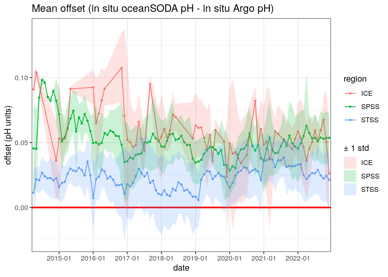
Offset between climatological Argo and climatological OceanSODA pH:
# Offset between climatological argo and climatological OceanSODA pH

argo_OceanSODA_SO_clim <- inner_join(argo_OceanSODA_SO_clim, nm_biomes)
argo_OceanSODA_SO_clim %>%
drop_na() %>%
ggplot() +
geom_point(aes(x = month, y = offset_clim, col = biome_name), size = 0.7, pch = 19) +
geom_hline(yintercept = 0, size = 1, col = 'red')+
scale_x_continuous(breaks = seq(1, 12, 1))+
labs(title = 'clim oceanSODA pH - clim Argo pH',
x = 'month',
y = 'offset (pH units)',
col = 'region')Mean offset between climatological OceanSODA pH and climatological Argo pH
mean_clim_offset <- argo_OceanSODA_SO_clim %>%
  group_by(month, biome_name) %>%
  summarise(mean_offset_clim = mean(offset_clim, na.rm = TRUE),
            std_offset_clim = sd(offset_clim, na.rm = TRUE))

mean_clim_offset %>%
  ggplot()+
  geom_point(aes(x = month, y = mean_offset_clim, col = biome_name))+
  geom_line(aes(x = month, y = mean_offset_clim, col = biome_name))+
  geom_hline(yintercept = 0, col = 'red') +
  geom_ribbon(aes(x = month,
                  ymin = mean_offset_clim - std_offset_clim,
                  ymax = mean_offset_clim + std_offset_clim,
                  group = biome_name,
                  fill = biome_name),
              alpha = 0.2) +
  scale_x_continuous(breaks = seq(1, 12, 1)) +
  labs(x = 'month',
       y = 'mean offset (pH units)',
       title = 'Mean offset (clim OceanSODA pH - clim Argo pH)',
       col = 'region',
fill = '± 1 std') 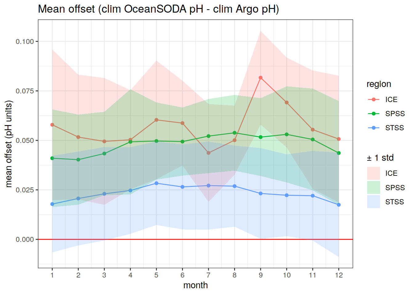
Mapped offset between climatological OceanSODA pH and climatological Argo pH
# bin the offsets for better plotting
# plot the offsets on a map of the Southern Ocean

argo_OceanSODA_SO_clim_2x2 <- argo_OceanSODA_SO_clim_2x2 %>%
  mutate(offset_clim_binned =
           cut(offset_clim,
               breaks = c(-Inf, -0.025, -0.005, 0.000, 0.005, 0.025, 0.035, 0.05, Inf))) %>%    # bin the offsets into intervals (create a discrete variable instead of continuous)
         # offset_clim_binned = as.factor(as.character(offset_clim_binned))) %>%
  drop_na()

map +
  geom_tile(data = argo_OceanSODA_SO_clim_2x2,
            aes(lon, lat, fill = offset_clim_binned)) +
  lims(y = c(-85, -30)) +
  scale_fill_brewer(palette = 'RdBu', drop = FALSE) +
  labs(x = 'lon',
       y = 'lat',
       fill = 'offset (pH units)',
       title = 'clim OceanSODA ph - clim Argo pH') +
  theme(legend.position = 'right')+
  facet_wrap(~month, ncol = 2)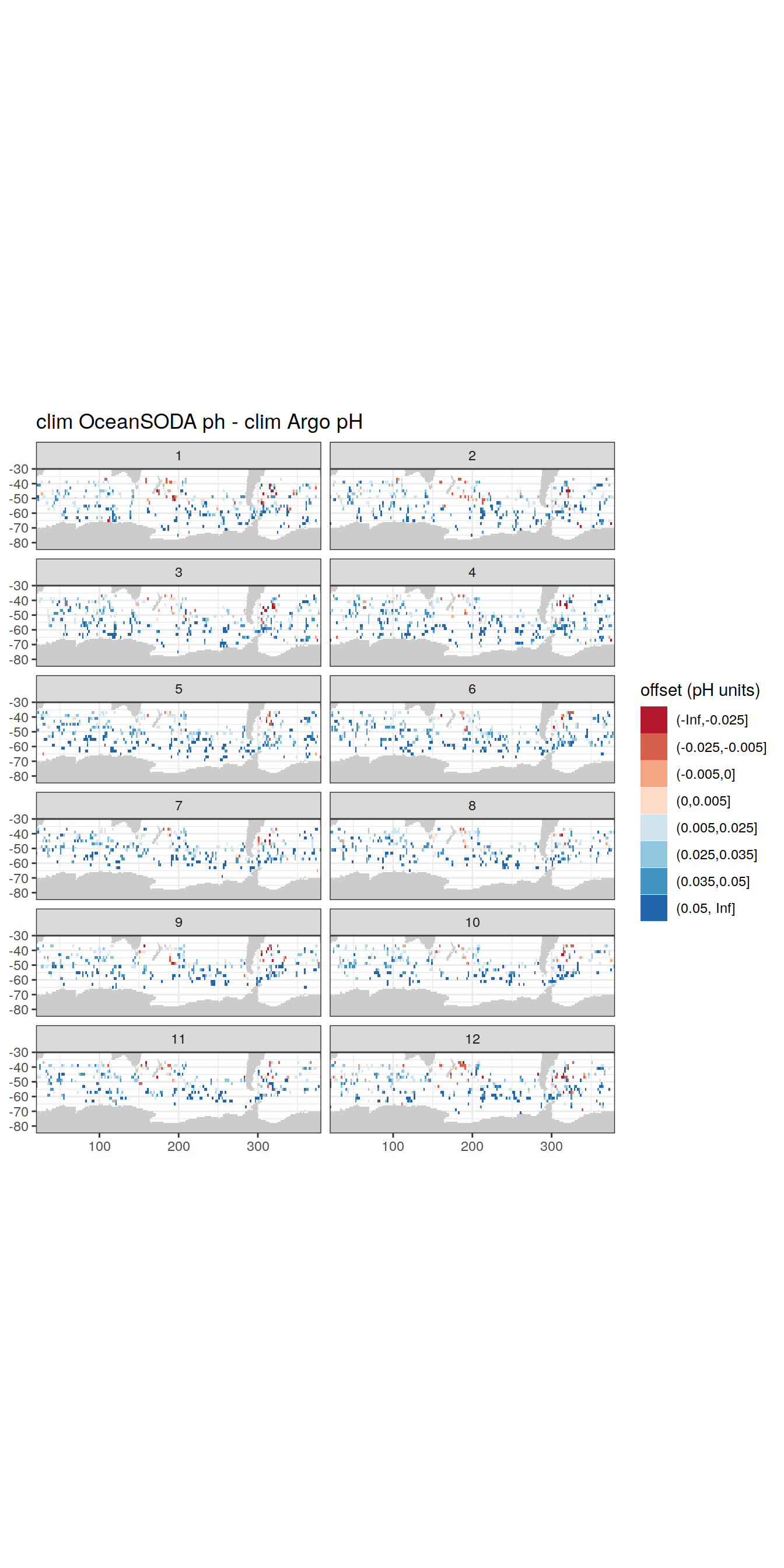
basemap(limits = -32, data = argo_OceanSODA_SO_clim_2x2) +   # change to polar projection
  geom_spatial_tile(data = argo_OceanSODA_SO_clim_2x2,
                    aes(x = lon,
                        y = lat,
                        fill = offset_clim_binned),
                    linejoin = 'mitre',
                    col = 'transparent',
                    detail = 60)+
  scale_fill_brewer(palette = 'RdBu', drop = FALSE)+
  theme(legend.position = 'right')+
  labs(x = 'lon',
       y = 'lat',
       fill = 'offset (pH units)',
       title = 'clim Ocean SODA pH - clim Argo pH')+
  facet_wrap(~month, ncol = 2)
Basin separation
Using full OceanSODA data (even where there is no Argo data) Each RECCAP biome (1, 2, 3) is separated into basins (Atlantic, Pacific, Indian)
basinmask <-
  read_csv(paste(path_emlr_utilities,
                 "basin_mask_WOA18.csv",
                 sep = ""),
           col_types = cols("MLR_basins" = col_character()))

basinmask <- basinmask %>%
  filter(MLR_basins == unique(basinmask$MLR_basins)[1]) %>%
  select(lon, lat, basin_AIP)

OceanSODA_SO <- inner_join(OceanSODA, nm_biomes)

OceanSODA_SO <- inner_join(OceanSODA_SO, basinmask) %>%
  mutate(year = year(date_OceanSODA),
         month = month(date_OceanSODA)) %>%
  mutate(date = format_ISO8601(date_OceanSODA, precision = 'ym')) %>%
  filter(year >= 2013)
# plot timeseries of monthly OceanSODA pH
OceanSODA_SO_clim_subregional <- OceanSODA_SO %>%
group_by(year, month, biome_name, basin_AIP) %>% # compute regional mean OceanSODA pH for the three biomes
summarise(ph = mean(ph_total, na.rm = TRUE)) %>%
ungroup()
# plot a timeseries of monthly average OceanSODA pH, per region and per basin
OceanSODA_SO_clim_subregional %>%
ggplot(aes(x = month,
y = ph,
group = year,
col = as.character(year)))+
geom_line()+
geom_point()+
scale_x_continuous(breaks = seq(1, 12, 2))+
facet_grid(biome_name~basin_AIP)+
labs(x = 'month',
y = 'pH in situ (total scale)',
title = 'monthly mean OceanSODA pH (Southern Ocean basins)',
col = 'year')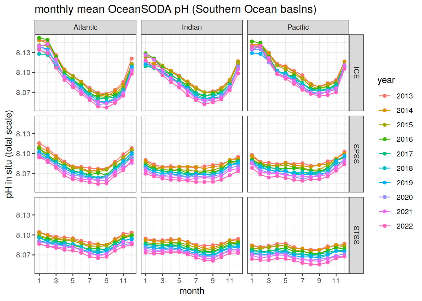
OceanSODA_SO_clim_subregional %>%
  ggplot(aes(x = year,
             y = ph,
             col = biome_name)) +
  facet_grid(month ~ basin_AIP) +
  geom_line() +
  geom_point() +
  labs(x = 'year',
       y = 'pH in situ (total scale)',
       title = 'monthly mean pH (Southern Ocean basins)',
       col = 'region')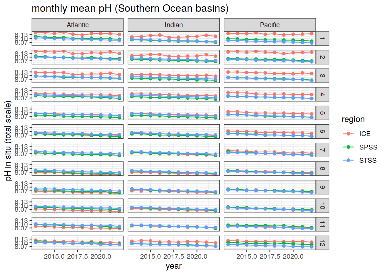
Longitudinal separation
Bin the pH data into 20º longitude bins (20º - 380º)
OceanSODA_SO_lon_binned <- OceanSODA_SO %>%
  mutate(lon = cut(lon, seq(20, 380, 20), seq(30, 370, 20)),
         lon = as.numeric(as.character(lon))
  ) %>%
  group_by(lon, year, month, biome_name) %>%
  summarise(
    OceanSODA_ph_binned = mean(ph_total, na.rm = TRUE)
  ) %>%
  ungroup()
OceanSODA_SO_lon_binned %>%
drop_na() %>%
ggplot(aes(x = month, y = OceanSODA_ph_binned, group = lon, col = as.factor(lon))) +
geom_line()+
geom_point()+
scale_x_continuous(breaks = seq(1, 12, 2))+
facet_grid(year~biome_name)+
labs(x = 'month',
y = 'OceanSODA pH',
col = 'longitude bin')
sessionInfo()R version 4.2.2 (2022-10-31)
Platform: x86_64-pc-linux-gnu (64-bit)
Running under: openSUSE Leap 15.5
Matrix products: default
BLAS: /usr/local/R-4.2.2/lib64/R/lib/libRblas.so
LAPACK: /usr/local/R-4.2.2/lib64/R/lib/libRlapack.so
locale:
[1] LC_CTYPE=en_US.UTF-8 LC_NUMERIC=C
[3] LC_TIME=en_US.UTF-8 LC_COLLATE=en_US.UTF-8
[5] LC_MONETARY=en_US.UTF-8 LC_MESSAGES=en_US.UTF-8
[7] LC_PAPER=en_US.UTF-8 LC_NAME=C
[9] LC_ADDRESS=C LC_TELEPHONE=C
[11] LC_MEASUREMENT=en_US.UTF-8 LC_IDENTIFICATION=C
attached base packages:
[1] stats graphics grDevices utils datasets methods base
other attached packages:
[1] metR_0.13.0 ggOceanMaps_1.3.4 ggspatial_1.1.7 lubridate_1.9.0
[5] timechange_0.1.1 argodata_0.1.0 forcats_0.5.2 stringr_1.5.0
[9] dplyr_1.1.3 purrr_1.0.2 readr_2.1.3 tidyr_1.3.0
[13] tibble_3.2.1 ggplot2_3.4.4 tidyverse_1.3.2 workflowr_1.7.0
loaded via a namespace (and not attached):
[1] fs_1.5.2 sf_1.0-9 bit64_4.0.5
[4] RColorBrewer_1.1-3 httr_1.4.4 rprojroot_2.0.3
[7] tools_4.2.2 backports_1.4.1 bslib_0.4.1
[10] utf8_1.2.2 R6_2.5.1 KernSmooth_2.23-20
[13] rgeos_0.5-9 DBI_1.2.2 colorspace_2.0-3
[16] raster_3.6-11 sp_1.5-1 withr_2.5.0
[19] tidyselect_1.2.0 processx_3.8.0 bit_4.0.5
[22] compiler_4.2.2 git2r_0.30.1 cli_3.6.1
[25] rvest_1.0.3 RNetCDF_2.6-1 xml2_1.3.3
[28] labeling_0.4.2 sass_0.4.4 checkmate_2.1.0
[31] scales_1.2.1 classInt_0.4-8 callr_3.7.3
[34] proxy_0.4-27 digest_0.6.30 rmarkdown_2.18
[37] pkgconfig_2.0.3 htmltools_0.5.8.1 highr_0.9
[40] dbplyr_2.2.1 fastmap_1.1.0 rlang_1.1.1
[43] readxl_1.4.1 rstudioapi_0.15.0 farver_2.1.1
[46] jquerylib_0.1.4 generics_0.1.3 jsonlite_1.8.3
[49] vroom_1.6.0 googlesheets4_1.0.1 magrittr_2.0.3
[52] Rcpp_1.0.10 munsell_0.5.0 fansi_1.0.3
[55] lifecycle_1.0.3 terra_1.7-65 stringi_1.7.8
[58] whisker_0.4 yaml_2.3.6 grid_4.2.2
[61] parallel_4.2.2 promises_1.2.0.1 crayon_1.5.2
[64] lattice_0.20-45 haven_2.5.1 hms_1.1.2
[67] knitr_1.41 ps_1.7.2 pillar_1.9.0
[70] codetools_0.2-18 reprex_2.0.2 glue_1.6.2
[73] evaluate_0.18 getPass_0.2-2 data.table_1.14.6
[76] modelr_0.1.10 vctrs_0.6.4 tzdb_0.3.0
[79] httpuv_1.6.6 cellranger_1.1.0 gtable_0.3.1
[82] assertthat_0.2.1 cachem_1.0.6 xfun_0.35
[85] broom_1.0.5 e1071_1.7-12 later_1.3.0
[88] viridisLite_0.4.1 class_7.3-20 googledrive_2.0.0
[91] gargle_1.2.1 memoise_2.0.1 units_0.8-0
[94] ellipsis_0.3.2