Climatology
Jens Daniel Müller
23 December, 2020
Last updated: 2020-12-23
Checks: 7 0
Knit directory: emlr_mod_preprocessing/
This reproducible R Markdown analysis was created with workflowr (version 1.6.2). The Checks tab describes the reproducibility checks that were applied when the results were created. The Past versions tab lists the development history.
Great! Since the R Markdown file has been committed to the Git repository, you know the exact version of the code that produced these results.
Great job! The global environment was empty. Objects defined in the global environment can affect the analysis in your R Markdown file in unknown ways. For reproduciblity it’s best to always run the code in an empty environment.
The command set.seed(20200707) was run prior to running the code in the R Markdown file. Setting a seed ensures that any results that rely on randomness, e.g. subsampling or permutations, are reproducible.
Great job! Recording the operating system, R version, and package versions is critical for reproducibility.
Nice! There were no cached chunks for this analysis, so you can be confident that you successfully produced the results during this run.
Great job! Using relative paths to the files within your workflowr project makes it easier to run your code on other machines.
Great! You are using Git for version control. Tracking code development and connecting the code version to the results is critical for reproducibility.
The results in this page were generated with repository version 37281b2. See the Past versions tab to see a history of the changes made to the R Markdown and HTML files.
Note that you need to be careful to ensure that all relevant files for the analysis have been committed to Git prior to generating the results (you can use wflow_publish or wflow_git_commit). workflowr only checks the R Markdown file, but you know if there are other scripts or data files that it depends on. Below is the status of the Git repository when the results were generated:
Ignored files:
    Ignored:    .Rproj.user/
Note that any generated files, e.g. HTML, png, CSS, etc., are not included in this status report because it is ok for generated content to have uncommitted changes.
These are the previous versions of the repository in which changes were made to the R Markdown (analysis/Climatology.Rmd) and HTML (docs/Climatology.html) files. If you’ve configured a remote Git repository (see ?wflow_git_remote), click on the hyperlinks in the table below to view the files as they were in that past version.
| File | Version | Author | Date | Message |
|---|---|---|---|---|
| html | e73a8c4 | jens-daniel-mueller | 2020-12-22 | Build site. |
| html | f66d4bc | jens-daniel-mueller | 2020-12-22 | Build site. |
| Rmd | 21b255e | jens-daniel-mueller | 2020-12-22 | rebuild after Jens revision |
| html | f6c7b00 | jens-daniel-mueller | 2020-12-21 | Build site. |
| Rmd | 0dcb5c3 | jens-daniel-mueller | 2020-12-21 | rebuild after Jens revision |
1 Read nc file
Here we used annual output of cmorized (1x1) model with variable forcing (RECCAP2 RunA) in year 2007 as the predictor climatology. Predictors include:
- Salinity (sal)
- Potential temperature (theta, not predictor, used for temperature calculation)
- In-situ temperature (temp, calculated)
- DIC (tco2)
- ALK (talk)
- oxygen
- AOU (calculated)
- nitrate
- phosphate
- silicate
# read in RECCAP2 RunA file
climatology_temp <- tidync(paste(
  path_cmorized,
  "RECCAP2_RunA.nc",
  sep = ""
))

# read-in 2007 as tibble
climatology <- climatology_temp %>%
  hyper_filter(time_ann = time_ann == 10036) %>%
  hyper_tibble()

# convert data variable to year
climatology <- climatology %>%
  mutate(year = format(as.Date(climatology$time_ann, origin = '1980-01-01'), "%Y"),
         year = as.numeric(year)) %>%
  select(-time_ann)

# select annual cmorized 2007 as climatology
climatology <- climatology %>%
  select(-epc) %>%
  rename(
    sal = so,
    THETA = thetao,
    tco2 = dissic,
    talk = talk,
    oxygen = o2,
    nitrate = no3,
    phosphate = po4,
    silicate = si
  ) %>%
  mutate(lon = if_else(lon < 20, lon + 360, lon)) %>%
  mutate(depth = round(depth))

rm(climatology_temp)
2 Apply basin mask
# use only three basin to assign general basin mask
# ie this is not specific to the MLR fitting
basinmask <- basinmask %>%
  filter(MLR_basins == "2") %>%
  select(lat, lon, basin_AIP)

# restrict predictor fields to basin mask grid
climatology <- inner_join(climatology, basinmask)
3 In-situ temperature
In-situ temperature was calculated as input paramter for AOU calculation.
climatology <- climatology %>%
  mutate(temp = gsw_pt_from_t(
    SA = sal,
    t = THETA,
    p = 10.1325,
    p_ref = depth
  ))
Example profile from North Atlantic Ocean.
climatology %>%
  filter(lat == params_global$lat_Atl_profile,
         lon == params_global$lon_Atl_section) %>%
  ggplot() +
  geom_line(aes(temp, depth, col = "insitu")) +
  geom_point(aes(temp, depth, col = "insitu")) +
  geom_line(aes(THETA, depth, col = "theta")) +
  geom_point(aes(THETA, depth, col = "theta")) +
  scale_y_reverse() +
  scale_color_brewer(palette = "Dark2", name = "Scale")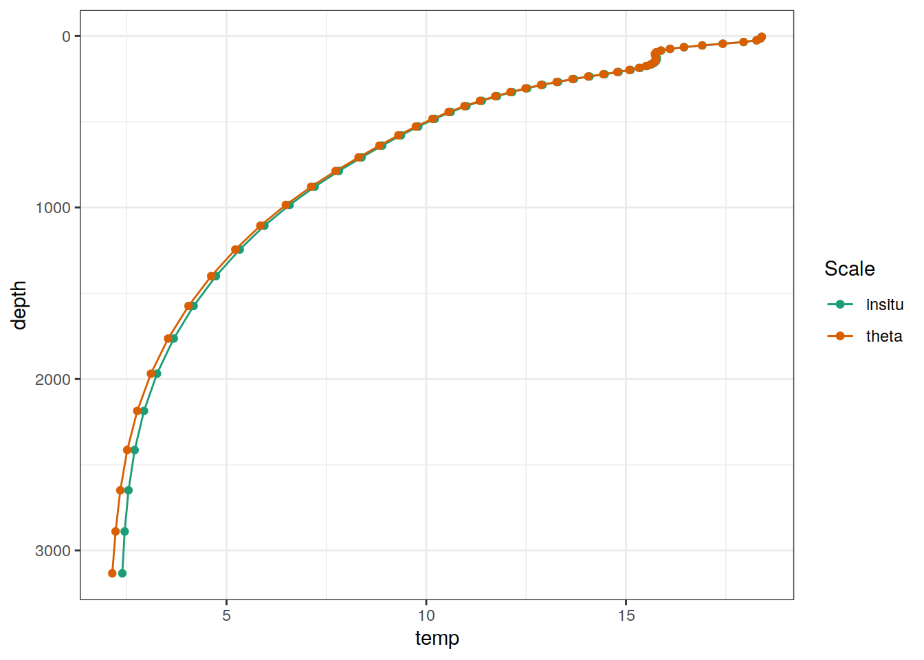
| Version | Author | Date |
|---|---|---|
| f6c7b00 | jens-daniel-mueller | 2020-12-21 |
4 Unit conversion
Model results are given in [mol m-3], whereas GLODAP data are in [µmol kg-1].
For comparison, model results were converted from [mol m-3] to [µmol kg-1]
# unit conversion from mol/m3 to µmol/kg
climatology <- climatology %>%
  mutate(
    rho = gsw_pot_rho_t_exact(
      SA = sal,
      t = temp,
      p = depth,
      p_ref = 10.1325
    ),
    tco2 = tco2 * (1e+06 / rho),
    talk = talk * (1e+06 / rho),
    oxygen = oxygen * (1e+06 / rho),
    nitrate = nitrate * (1e+06 / rho),
    phosphate = phosphate * (1e+06 / rho),
    silicate = silicate * (1e+06 / rho)
  )
5 AOU calculation
climatology <- climatology %>%
mutate(
oxygen_sat_m3 = gas_satconc(
S = sal,
t = temp,
P = 1.013253,
species = "O2"
),
oxygen_sat_kg = oxygen_sat_m3 * (1e+3 / rho),
AOU = oxygen_sat_kg - oxygen
) %>%
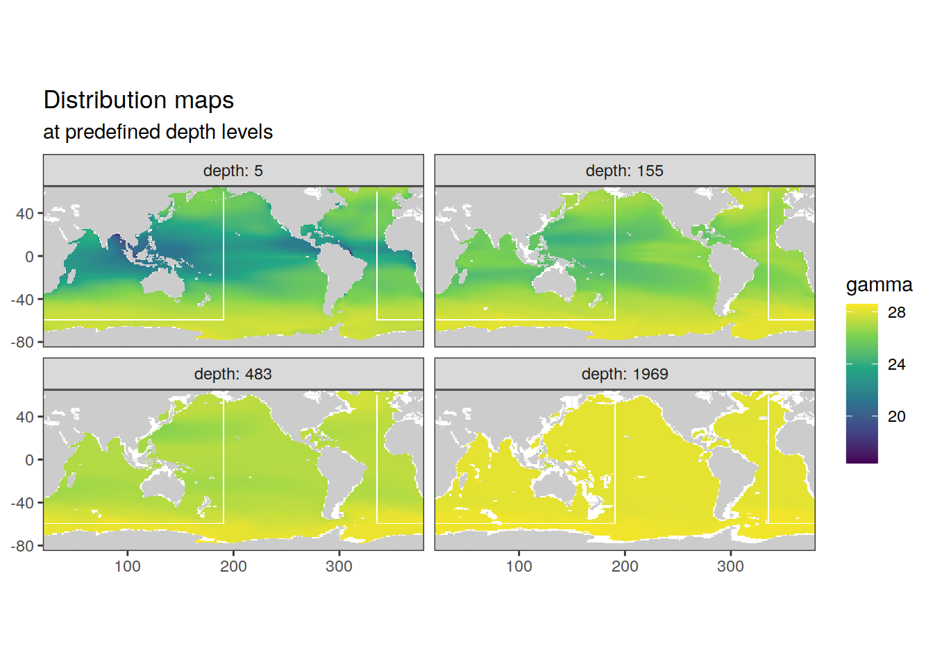
select(-oxygen_sat_kg,-oxygen_sat_m3)6 Neutral density calculation
Neutral density gamma was calculated with a Python script provided by Serazin et al (2011), which performs a polynomial approximation of the original gamma calculation.
# calculate pressure from depth
climatology <- climatology %>%
  mutate(CTDPRS = gsw_p_from_z(-depth,
                               lat))

# rename variables according to python script
climatology_gamma_prep <- climatology %>%
  rename(LATITUDE = lat,
         LONGITUDE = lon,
         SALNTY = sal)

# load python scripts
source_python(paste(
  path_functions,
  "python_scripts/Gamma_GLODAP_python.py",
  sep = ""
))

# calculate gamma
climatology_gamma_calc <-
  calculate_gamma(climatology_gamma_prep)

# reverse variable naming
climatology <- climatology_gamma_calc %>%
  select(-c(CTDPRS, THETA)) %>%
  rename(
    lat = LATITUDE,
    lon = LONGITUDE,
    sal = SALNTY,
    gamma  = GAMMA
  )

climatology <- as_tibble(climatology)

rm(climatology_gamma_calc, climatology_gamma_prep)
7 Write file
# select relevant columns
climatology <- climatology %>%
select(-c(year, rho))
# write csv file
climatology %>%
write_csv(paste(path_preprocessing,
"climatology_runA_2007.csv",
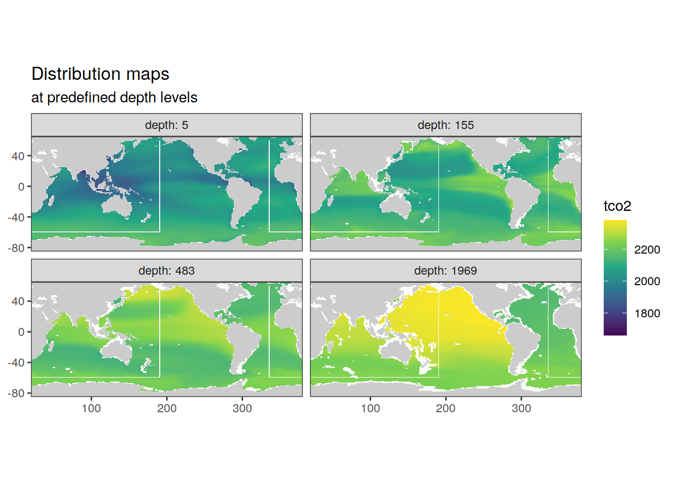
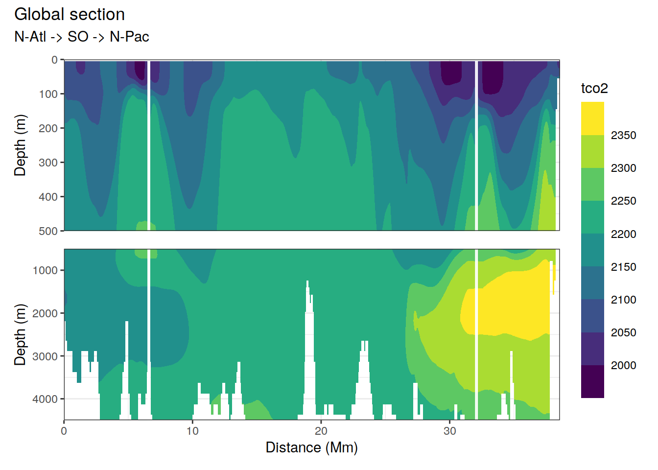
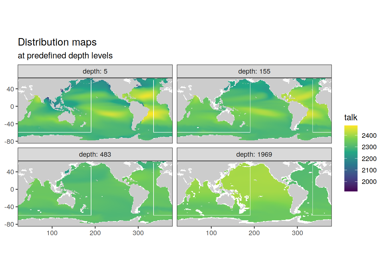
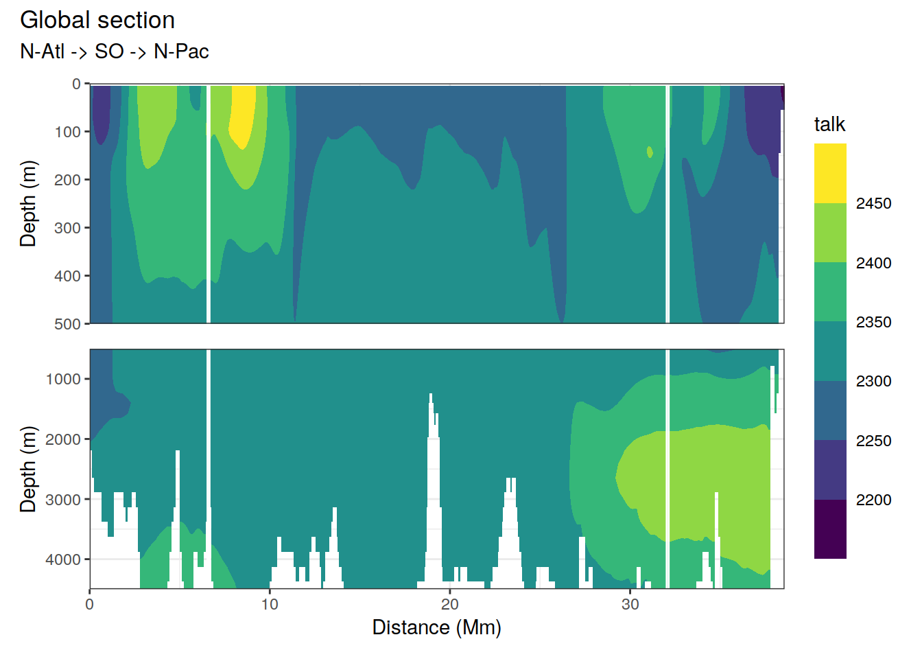
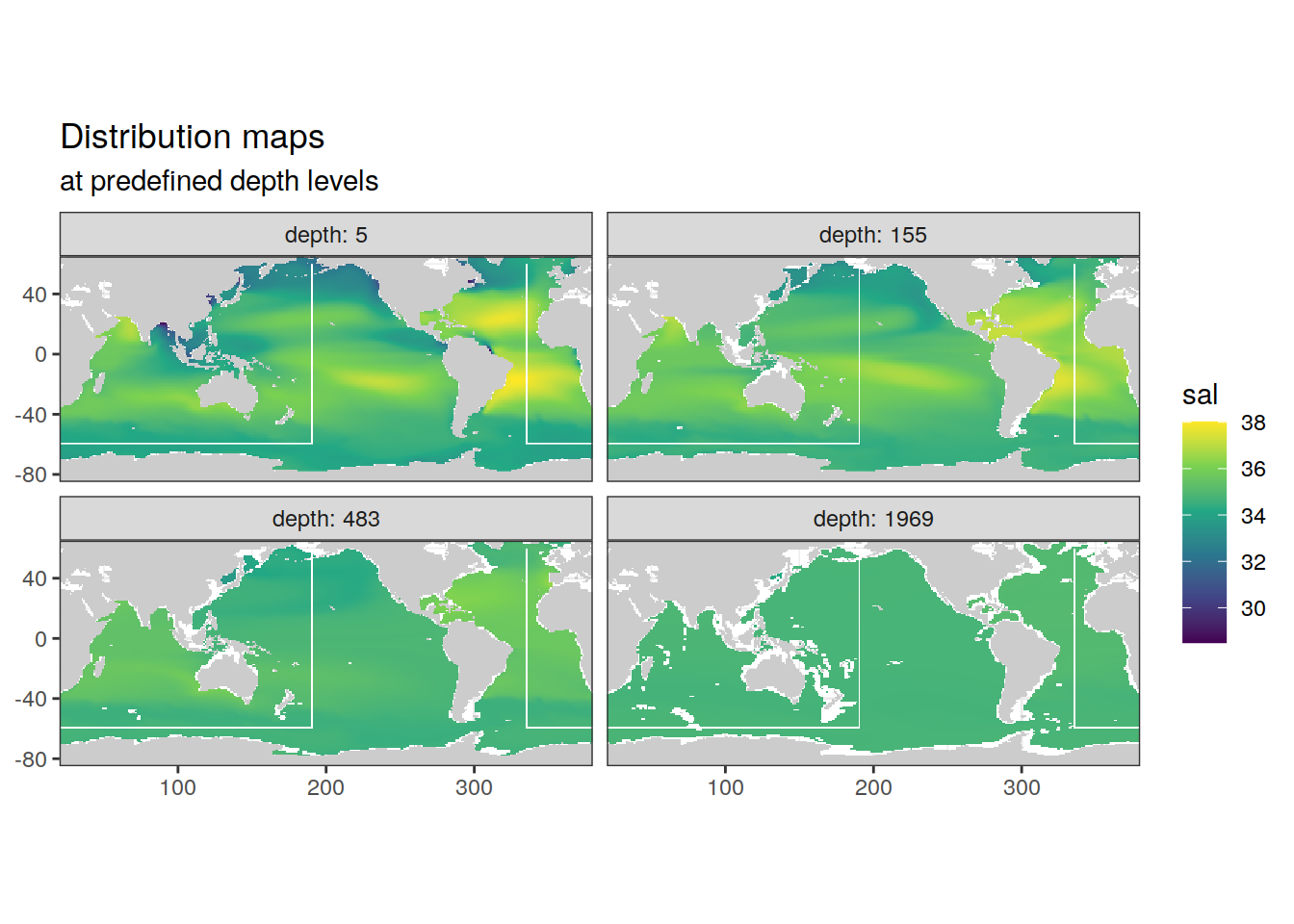
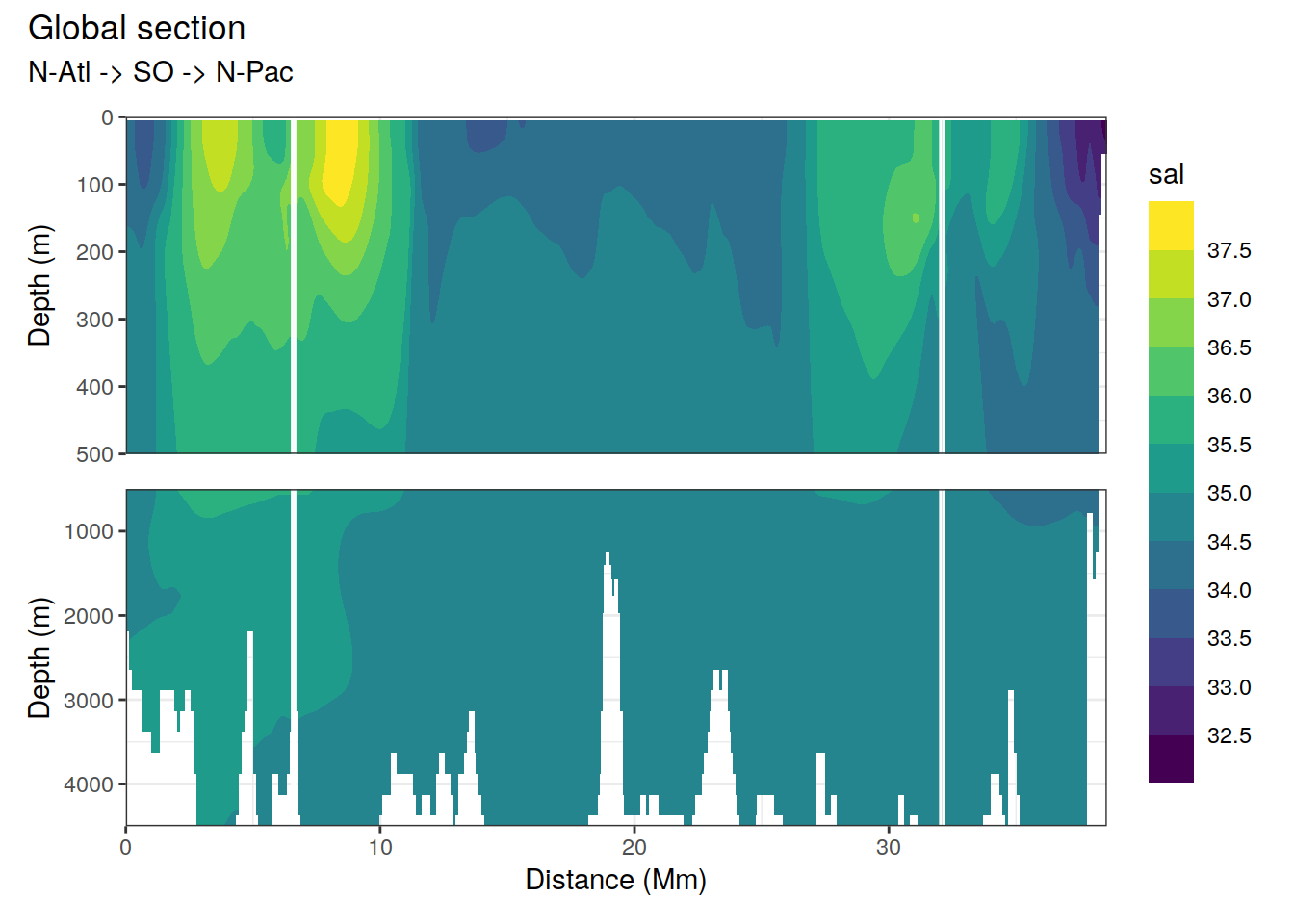
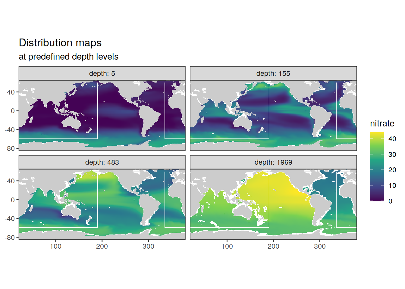
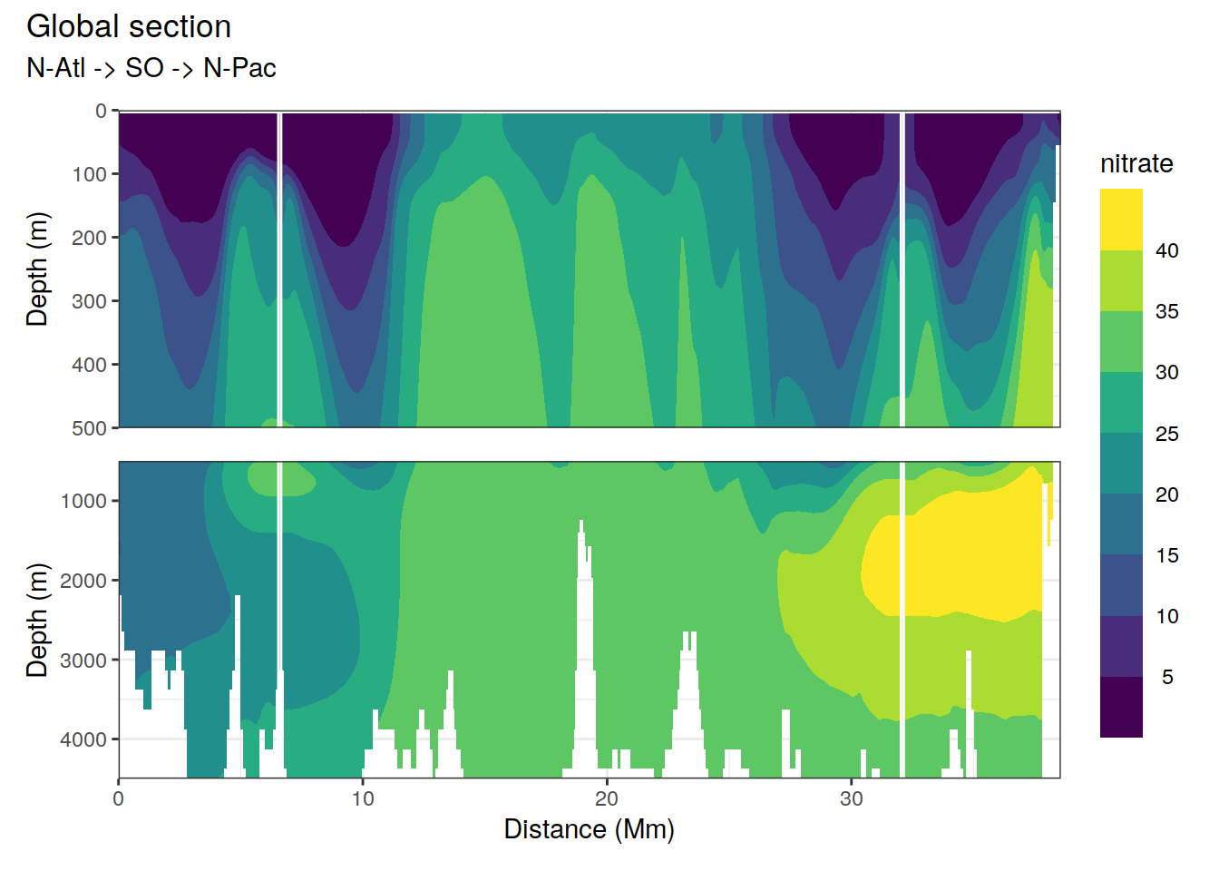
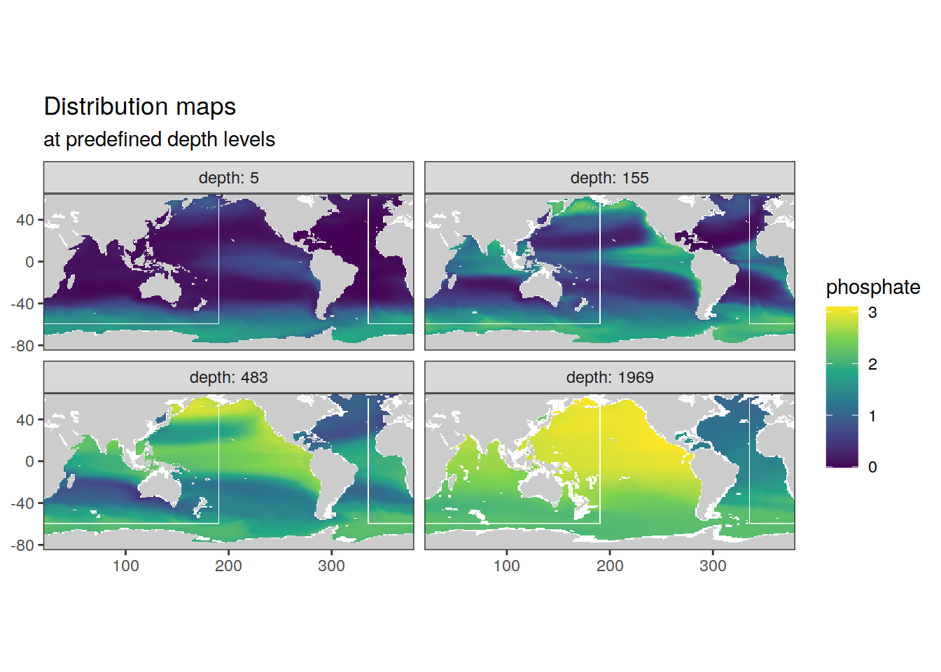
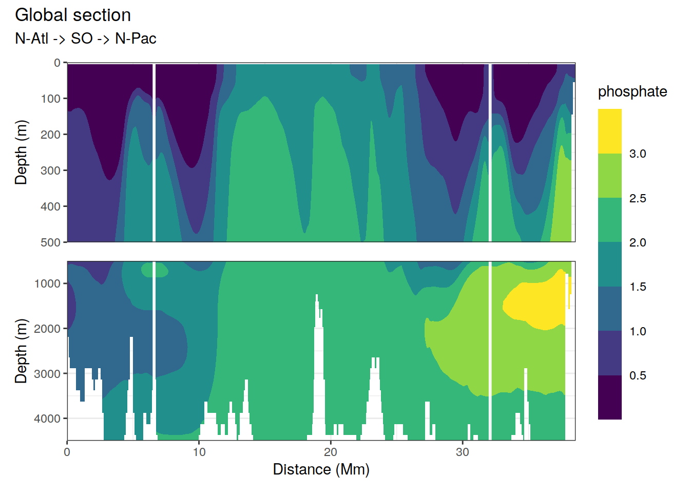
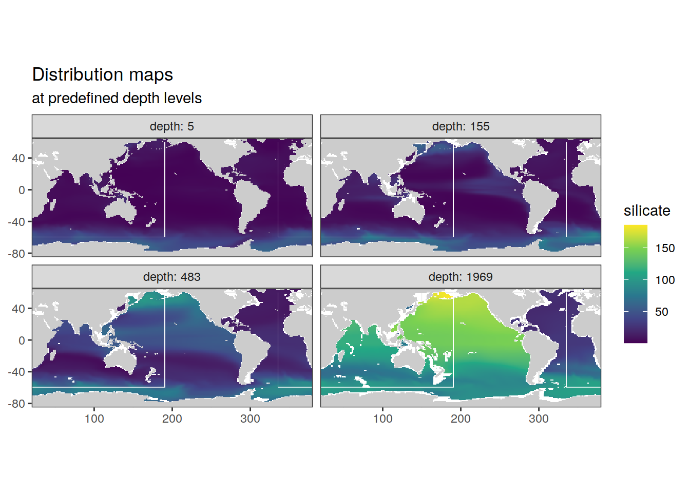
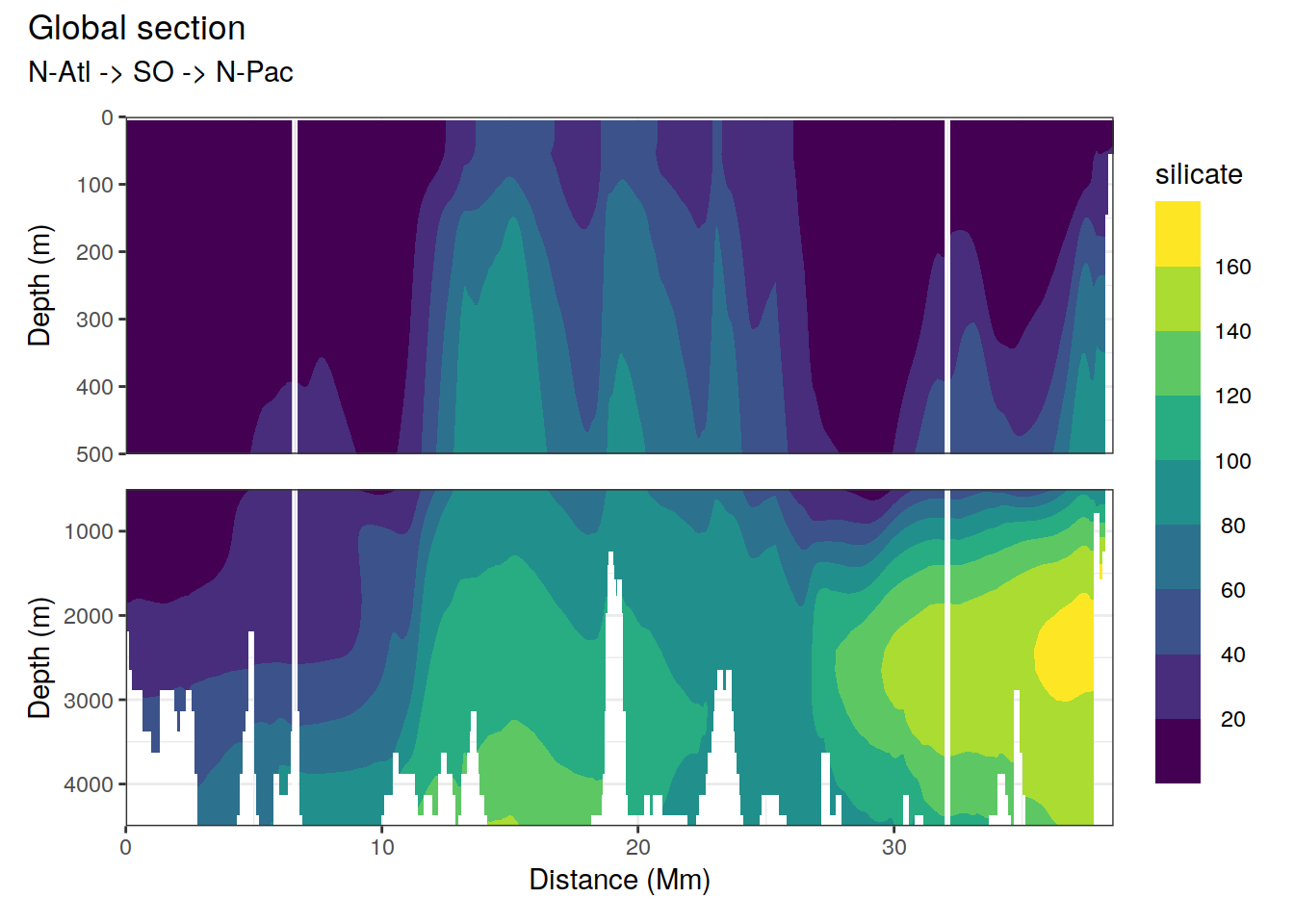
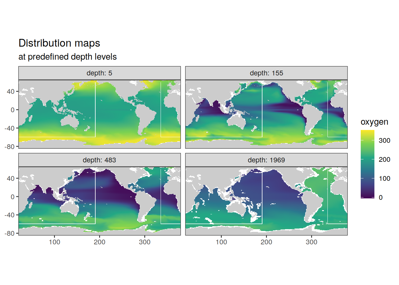
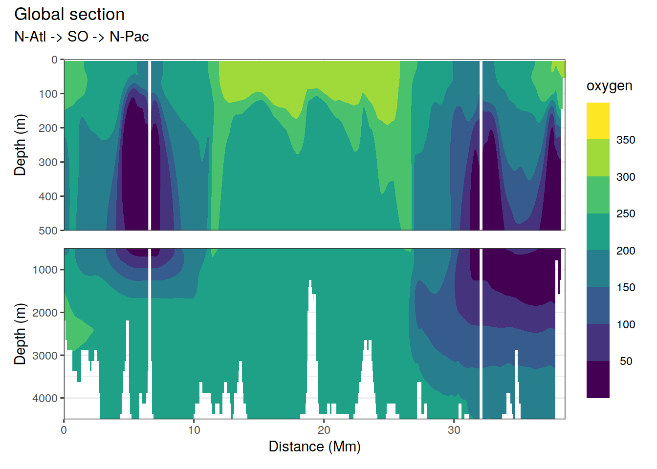
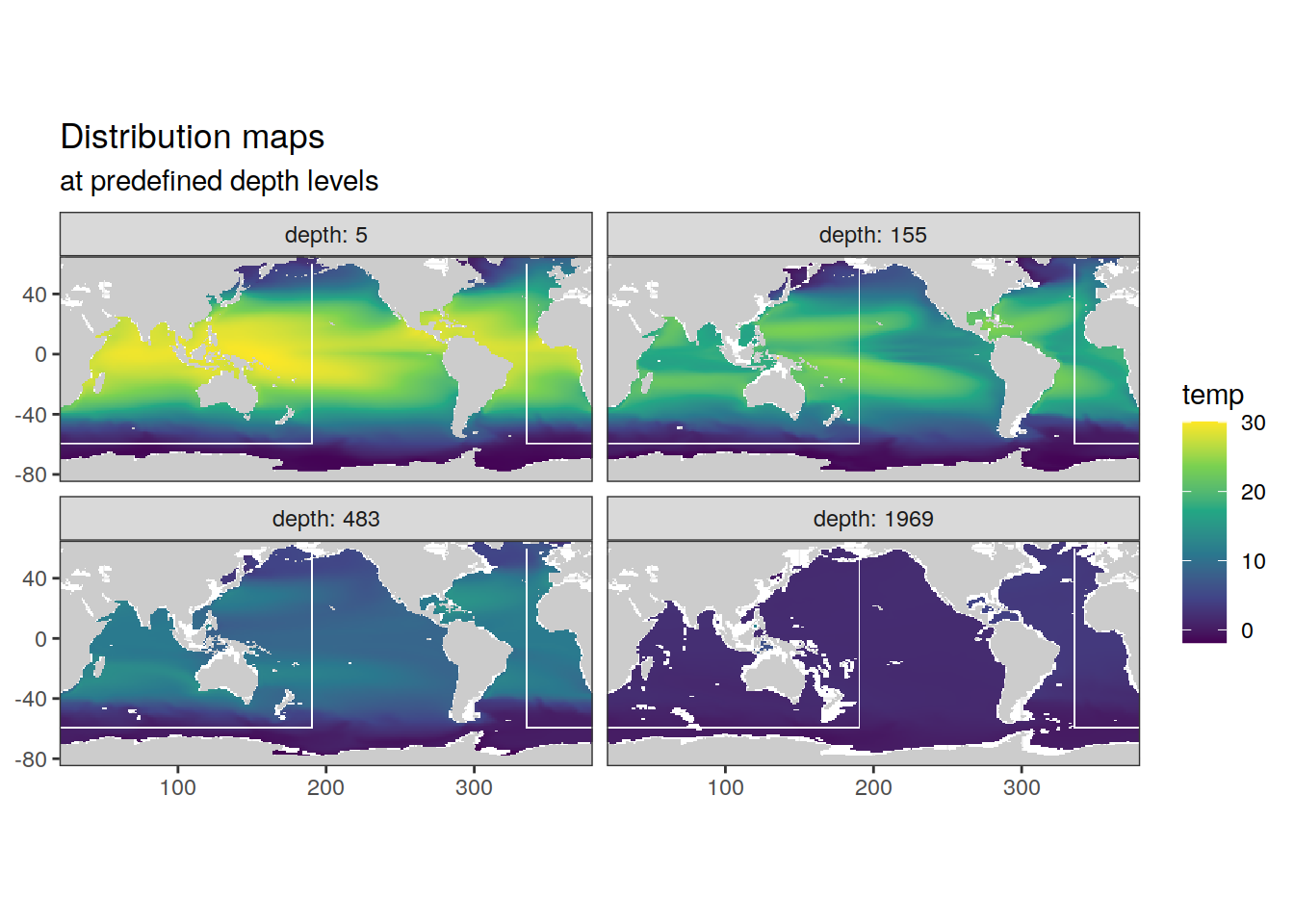
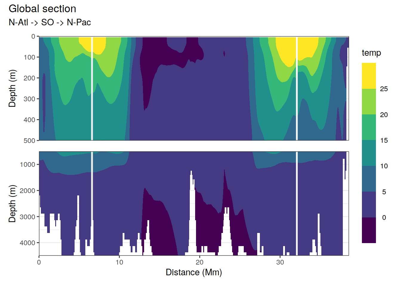
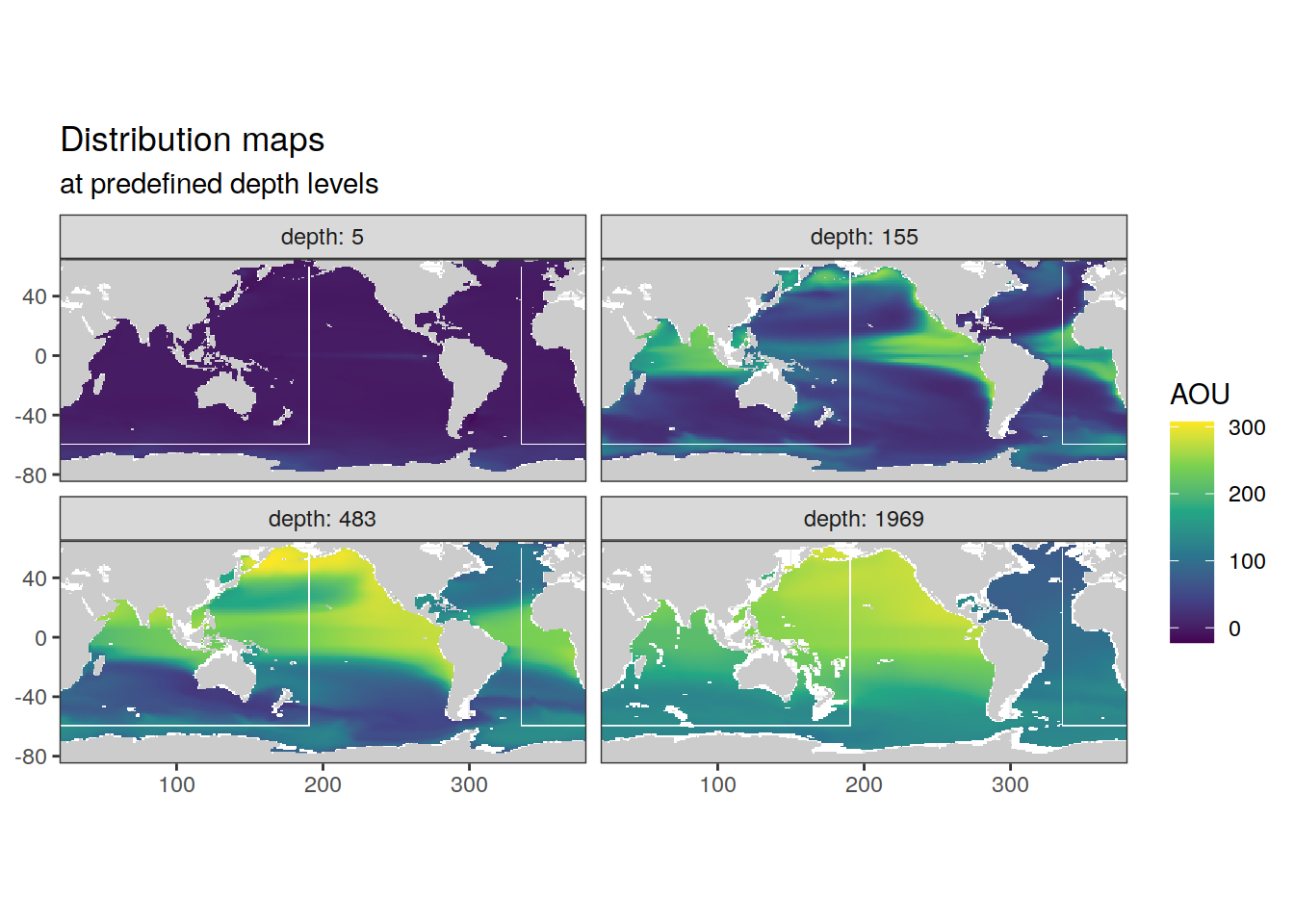
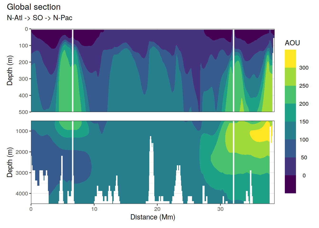
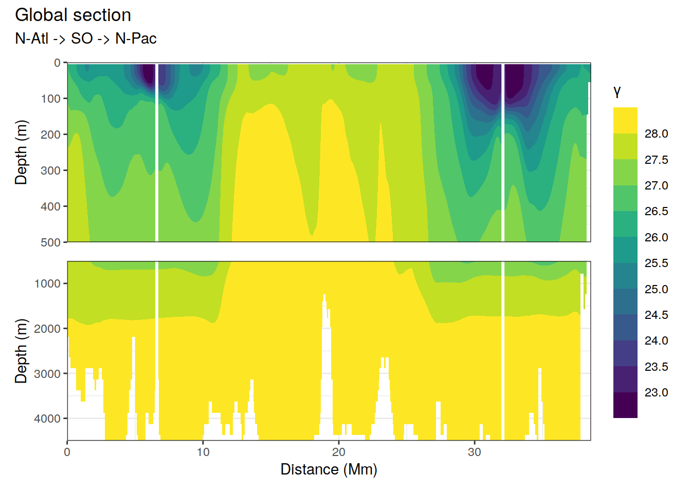
sep = ""))8 Plots
Below, following subsets of the climatology are plotted for all relevant predictors:
- Horizontal planes at 4 depth levels
- Global section along track indicated by white lines in maps.
# define plotting variables
vars <- c(
  "tco2",
  "talk",
  "sal",
  "nitrate",
  "phosphate",
  "silicate",
  "oxygen",
  "temp",
  "AOU",
  "gamma"
)

# i_var <- vars[1]

for (i_var in vars) {
  # plot maps

  print(p_map_climatology(df = climatology,
                          var = i_var))

  # plot sections

  print(p_section_global(df = climatology,
                         var = i_var))

}
| Version | Author | Date |
|---|---|---|
| f6c7b00 | jens-daniel-mueller | 2020-12-21 |
| Version | Author | Date |
|---|---|---|
| f6c7b00 | jens-daniel-mueller | 2020-12-21 |
| Version | Author | Date |
|---|---|---|
| f6c7b00 | jens-daniel-mueller | 2020-12-21 |
| Version | Author | Date |
|---|---|---|
| f6c7b00 | jens-daniel-mueller | 2020-12-21 |
| Version | Author | Date |
|---|---|---|
| f6c7b00 | jens-daniel-mueller | 2020-12-21 |
| Version | Author | Date |
|---|---|---|
| f6c7b00 | jens-daniel-mueller | 2020-12-21 |
| Version | Author | Date |
|---|---|---|
| f6c7b00 | jens-daniel-mueller | 2020-12-21 |
| Version | Author | Date |
|---|---|---|
| f6c7b00 | jens-daniel-mueller | 2020-12-21 |
| Version | Author | Date |
|---|---|---|
| f6c7b00 | jens-daniel-mueller | 2020-12-21 |
| Version | Author | Date |
|---|---|---|
| f6c7b00 | jens-daniel-mueller | 2020-12-21 |
| Version | Author | Date |
|---|---|---|
| f6c7b00 | jens-daniel-mueller | 2020-12-21 |
| Version | Author | Date |
|---|---|---|
| f6c7b00 | jens-daniel-mueller | 2020-12-21 |
| Version | Author | Date |
|---|---|---|
| f6c7b00 | jens-daniel-mueller | 2020-12-21 |
| Version | Author | Date |
|---|---|---|
| f6c7b00 | jens-daniel-mueller | 2020-12-21 |
| Version | Author | Date |
|---|---|---|
| f6c7b00 | jens-daniel-mueller | 2020-12-21 |
| Version | Author | Date |
|---|---|---|
| f6c7b00 | jens-daniel-mueller | 2020-12-21 |
| Version | Author | Date |
|---|---|---|
| f6c7b00 | jens-daniel-mueller | 2020-12-21 |
| Version | Author | Date |
|---|---|---|
| f6c7b00 | jens-daniel-mueller | 2020-12-21 |
| Version | Author | Date |
|---|---|---|
| f6c7b00 | jens-daniel-mueller | 2020-12-21 |
| Version | Author | Date |
|---|---|---|
| f6c7b00 | jens-daniel-mueller | 2020-12-21 |
sessionInfo()R version 4.0.3 (2020-10-10)
Platform: x86_64-pc-linux-gnu (64-bit)
Running under: openSUSE Leap 15.1
Matrix products: default
BLAS: /usr/local/R-4.0.3/lib64/R/lib/libRblas.so
LAPACK: /usr/local/R-4.0.3/lib64/R/lib/libRlapack.so
locale:
[1] LC_CTYPE=en_US.UTF-8 LC_NUMERIC=C
[3] LC_TIME=en_US.UTF-8 LC_COLLATE=en_US.UTF-8
[5] LC_MONETARY=en_US.UTF-8 LC_MESSAGES=en_US.UTF-8
[7] LC_PAPER=en_US.UTF-8 LC_NAME=C
[9] LC_ADDRESS=C LC_TELEPHONE=C
[11] LC_MEASUREMENT=en_US.UTF-8 LC_IDENTIFICATION=C
attached base packages:
[1] stats graphics grDevices utils datasets methods base
other attached packages:
[1] marelac_2.1.10 shape_1.4.5 geosphere_1.5-10 oce_1.2-0
[5] gsw_1.0-5 testthat_3.0.1 reticulate_1.18 tidync_0.2.4
[9] metR_0.8.0 scico_1.2.0 patchwork_1.1.0 collapse_1.4.2
[13] forcats_0.5.0 stringr_1.4.0 dplyr_1.0.2 purrr_0.3.4
[17] readr_1.4.0 tidyr_1.1.2 tibble_3.0.4 ggplot2_3.3.2
[21] tidyverse_1.3.0 workflowr_1.6.2
loaded via a namespace (and not attached):
[1] fs_1.5.0 lubridate_1.7.9 RColorBrewer_1.1-2
[4] httr_1.4.2 rprojroot_2.0.2 tools_4.0.3
[7] backports_1.2.1 R6_2.5.0 DBI_1.1.0
[10] colorspace_2.0-0 withr_2.3.0 sp_1.4-4
[13] tidyselect_1.1.0 compiler_4.0.3 git2r_0.27.1
[16] cli_2.2.0 rvest_0.3.6 RNetCDF_2.4-2
[19] xml2_1.3.2 isoband_0.2.3 labeling_0.4.2
[22] scales_1.1.1 checkmate_2.0.0 rappdirs_0.3.1
[25] digest_0.6.27 rmarkdown_2.5 pkgconfig_2.0.3
[28] htmltools_0.5.0 dbplyr_1.4.4 rlang_0.4.9
[31] readxl_1.3.1 rstudioapi_0.13 farver_2.0.3
[34] generics_0.1.0 jsonlite_1.7.2 magrittr_2.0.1
[37] ncmeta_0.3.0 Matrix_1.2-18 Rcpp_1.0.5
[40] munsell_0.5.0 fansi_0.4.1 lifecycle_0.2.0
[43] stringi_1.5.3 whisker_0.4 yaml_2.2.1
[46] grid_4.0.3 blob_1.2.1 parallel_4.0.3
[49] promises_1.1.1 crayon_1.3.4 lattice_0.20-41
[52] haven_2.3.1 hms_0.5.3 seacarb_3.2.14
[55] knitr_1.30 pillar_1.4.7 reprex_0.3.0
[58] glue_1.4.2 evaluate_0.14 RcppArmadillo_0.10.1.2.0
[61] data.table_1.13.4 modelr_0.1.8 vctrs_0.3.6
[64] httpuv_1.5.4 cellranger_1.1.0 gtable_0.3.0
[67] assertthat_0.2.1 xfun_0.19 broom_0.7.3
[70] RcppEigen_0.3.3.9.1 later_1.1.0.1 viridisLite_0.3.0
[73] ncdf4_1.17 ellipsis_0.3.1