Annual cmorized Cant field
Jens Daniel Müller
19 December, 2020
Last updated: 2020-12-19
Checks: 7 0
Knit directory: model/
This reproducible R Markdown analysis was created with workflowr (version 1.6.2). The Checks tab describes the reproducibility checks that were applied when the results were created. The Past versions tab lists the development history.
Great! Since the R Markdown file has been committed to the Git repository, you know the exact version of the code that produced these results.
Great job! The global environment was empty. Objects defined in the global environment can affect the analysis in your R Markdown file in unknown ways. For reproduciblity it’s best to always run the code in an empty environment.
The command set.seed(20200707) was run prior to running the code in the R Markdown file. Setting a seed ensures that any results that rely on randomness, e.g. subsampling or permutations, are reproducible.
Great job! Recording the operating system, R version, and package versions is critical for reproducibility.
Nice! There were no cached chunks for this analysis, so you can be confident that you successfully produced the results during this run.
Great job! Using relative paths to the files within your workflowr project makes it easier to run your code on other machines.
Great! You are using Git for version control. Tracking code development and connecting the code version to the results is critical for reproducibility.
The results in this page were generated with repository version 39657d6. See the Past versions tab to see a history of the changes made to the R Markdown and HTML files.
Note that you need to be careful to ensure that all relevant files for the analysis have been committed to Git prior to generating the results (you can use wflow_publish or wflow_git_commit). workflowr only checks the R Markdown file, but you know if there are other scripts or data files that it depends on. Below is the status of the Git repository when the results were generated:
Ignored files:
    Ignored:    .Rhistory
    Ignored:    .Rproj.user/

Unstaged changes:
    Modified:   analysis/_site.yml
    Deleted:    analysis/read_GLODAPv2_2016_MappedClimatologies.Rmd
    Deleted:    analysis/read_GLODAPv2_2020.Rmd
    Deleted:    analysis/read_Gruber_2019_Cant.Rmd
    Deleted:    analysis/read_Sabine_2004_Cant.Rmd
    Deleted:    analysis/read_World_Ocean_Atlas_2018.Rmd
    Modified:   code/Workflowr_project_managment.R
Note that any generated files, e.g. HTML, png, CSS, etc., are not included in this status report because it is ok for generated content to have uncommitted changes.
These are the previous versions of the repository in which changes were made to the R Markdown (analysis/cmorized_Cant.Rmd) and HTML (docs/cmorized_Cant.html) files. If you’ve configured a remote Git repository (see ?wflow_git_remote), click on the hyperlinks in the table below to view the files as they were in that past version.
| File | Version | Author | Date | Message |
|---|---|---|---|---|
| Rmd | 39657d6 | Donghe-Zhu | 2020-12-19 | rebuild final cleaned version |
| html | c3590c6 | Donghe-Zhu | 2020-12-18 | Build site. |
| Rmd | 0e3fd97 | Donghe-Zhu | 2020-12-18 | rebuild final cleaned version |
| html | 7c12d28 | Donghe-Zhu | 2020-12-18 | Build site. |
| Rmd | 1b06f98 | Donghe-Zhu | 2020-12-18 | rebuild final cleaned version |
1 Calculate annual Cant field
1.1 Read in cmorized RunA file
# read in cmorized variable forcing model file
A_annual <- tidync(paste(path_cmorized,
                         "RECCAP2_RunA.nc",
                         sep = ""))

A_annual <- A_annual %>% hyper_tibble()

# harmonize column names and coordinates
A_annual <- A_annual  %>%
  select(year = time_ann, lon, lat, depth, tco2_A = dissic, sal = so, theta = thetao) %>%
  # select annual value in year of 2007
  mutate(year = (year - 181) / 365 + 1980) %>%
  mutate(lon = if_else(lon < 20, lon + 360, lon))

# calculate model temperature
A_annual <- A_annual %>%
  mutate(temp = gsw_pt_from_t(
    SA = sal,
    t = theta,
    p = 10.1325,
    p_ref = depth
  ))

# unit transfer from mol/m3 to µmol/kg
A_annual <- A_annual %>%
  mutate(
    rho = gsw_pot_rho_t_exact(
      SA = sal,
      t = temp,
      p = depth,
      p_ref = 10.1325
    ),
    tco2_A = tco2_A * (1000000 / rho)
  ) %>%
  select(year, lon, lat, depth, tco2_A)
1.2 Read in cmorized RunB file
# read in cmorized variable forcing model file
B_annual <- tidync(paste(path_cmorized,
                         "RECCAP2_RunB.nc",
                         sep = ""))

B_annual <- B_annual %>% hyper_tibble()

# harmonize column names and coordinates
B_annual <- B_annual  %>%
  select(year = time_ann, lon, lat, depth, tco2_B = dissic, sal = so, theta = thetao) %>%
  # select annual value in year of 2007
  mutate(year = (year - 181) / 365 + 1980) %>%
  mutate(lon = if_else(lon < 20, lon + 360, lon))

# calculate model temperature
B_annual <- B_annual %>%
  mutate(temp = gsw_pt_from_t(
    SA = sal,
    t = theta,
    p = 10.1325,
    p_ref = depth
  ))

# unit transfer from mol/m3 to µmol/kg
B_annual <- B_annual %>%
  mutate(
    rho = gsw_pot_rho_t_exact(
      SA = sal,
      t = temp,
      p = depth,
      p_ref = 10.1325
    ),
    tco2_B = tco2_B * (1000000 / rho)
  ) %>%
  select(year, lon, lat, depth, tco2_B)

# join files and calculate Cant field
cant_annual <- inner_join(A_annual, B_annual) %>%
  mutate(cant = tco2_A - tco2_B)

rm(A_annual, B_annual)
1.3 Apply basin mask
# use only three basin to assign general basin mask
# ie this is not specific to the MLR fitting
basinmask <- basinmask %>%
  filter(MLR_basins == "2") %>%
  select(lat, lon, basin_AIP)

# restrict Cant field to basin mask grid
cant_annual <- inner_join(cant_annual, basinmask)
1.4 Calculate dCant for year 1994 - 2007
cant_annual_1994 <- cant_annual %>%
  filter(year == 1994) %>%
  select(-c(tco2_A, tco2_B, year)) %>%
  rename(cant_1994 = cant)

cant_annual_2007 <- cant_annual %>%
  filter(year == 2007) %>%
  select(-c(tco2_A, tco2_B, year)) %>%
  rename(cant_2007 = cant)

dcant_gruber <- left_join(cant_annual_1994, cant_annual_2007) %>%
  mutate(dcant = cant_2007 - cant_1994)

rm(cant_annual_1994, cant_annual_2007)
1.5 Write Cant files
# write combined Cant file
cant_annual %>%
  write_csv(paste(
    path_preprocessing,
    "cant_annual_field/cant_all_years.csv",
    sep = ""
  ))

# write annual Cant files
years <- c(1982:2019)
for (i_year in years) {

 # i_year = years[1]
  cant_annual_year <- cant_annual %>%
    filter(year == i_year) %>%
    select(year, lon, lat, depth, cant)

  cant_annual_year %>%
    write_csv(paste(path_preprocessing,
                    "cant_annual_field/cant_", i_year, ".csv",
                    sep = ""))
}

# write dCant gruber file
dcant_gruber %>%
  write_csv(paste(
    path_preprocessing,
    "cant_annual_field/dcant_gruber.csv",
    sep = ""
  ))

rm(cant_annual_year)
2 Zonal mean section
# Zonal mean section for Cant
cant_annual_zonal <- cant_annual %>%
  select(-c(lon, tco2_A, tco2_B)) %>%
  fgroup_by(lat, depth, year, basin_AIP) %>% {
    add_vars(
      fgroup_vars(., "unique"),
      fmean(., keep.group_vars = FALSE) %>% add_stub(pre = FALSE, "_mean"),
      fsd(., keep.group_vars = FALSE) %>% add_stub(pre = FALSE, "_sd")
    )
  }

# Zonal mean section for dCant
dcant_gruber_zonal <- dcant_gruber %>%
  select(-c(lon, cant_1994, cant_2007)) %>%
  fgroup_by(lat, depth, basin_AIP) %>% {
    add_vars(
      fgroup_vars(., "unique"),
      fmean(., keep.group_vars = FALSE) %>% add_stub(pre = FALSE, "_mean"),
      fsd(., keep.group_vars = FALSE) %>% add_stub(pre = FALSE, "_sd")
    )
  }
3 Column inventory
3.1 Calculation
# Calculate column inventory for Cant in year 2007
for (i_inventory_depth in params_global$inventory_depths) {
  # filter integration depth
  cant_annual_temp <- cant_annual %>%
    filter(year == 2007, depth <= i_inventory_depth)

  depth_level_volume <- tibble(depth = unique(cant_annual_temp$depth)) %>%
    arrange(depth)

  # determine depth level volume of each depth layer
  depth_level_volume <- depth_level_volume %>%
    mutate(
      layer_thickness_above = replace_na((depth - lag(depth)) / 2, 0),
      layer_thickness_below = replace_na((lead(depth) - depth) / 2, 0),
      layer_thickness = layer_thickness_above + layer_thickness_below
    ) %>%
    select(-c(layer_thickness_above,
              layer_thickness_below))

  cant_annual_temp <-
    full_join(cant_annual_temp, depth_level_volume)

  # calculate cant layer inventory
  cant_annual_temp <- cant_annual_temp %>%
    mutate(cant_layer_inv = cant * layer_thickness * 1.03) %>%
    select(-layer_thickness)

  # sum up layer inventories to column inventories
  cant_annual_inv_temp <- cant_annual_temp %>%
    group_by(lon, lat, basin_AIP) %>%
    summarise(cant_inv = sum(cant_layer_inv, na.rm = TRUE) / 1000) %>%
    ungroup()

  cant_annual_inv_temp <- cant_annual_inv_temp %>%
    mutate(inv_depth = i_inventory_depth)

  if (exists("cant_annual_inv")) {
    cant_annual_inv <- bind_rows(cant_annual_inv, cant_annual_inv_temp)
  }

  if (!exists("cant_annual_inv")) {
    cant_annual_inv <- cant_annual_inv_temp
  }
}

cant_annual_inv <- cant_annual_inv %>%
  filter(inv_depth == params_global$inventory_depth_standard)

rm(cant_annual_inv_temp, cant_annual_temp)

# Calculate column inventory for dCant
for (i_inventory_depth in params_global$inventory_depths) {
  # filter integration depth
  dcant_gruber_temp <- dcant_gruber %>%
    filter(depth <= i_inventory_depth)

  depth_level_volume <- tibble(depth = unique(dcant_gruber_temp$depth)) %>%
    arrange(depth)

  # determine depth level volume of each depth layer
  depth_level_volume <- depth_level_volume %>%
    mutate(
      layer_thickness_above = replace_na((depth - lag(depth)) / 2, 0),
      layer_thickness_below = replace_na((lead(depth) - depth) / 2, 0),
      layer_thickness = layer_thickness_above + layer_thickness_below
    ) %>%
    select(-c(layer_thickness_above,
              layer_thickness_below))

  dcant_gruber_temp <-
    full_join(dcant_gruber_temp, depth_level_volume)

  # calculate cant layer inventory
  dcant_gruber_temp <- dcant_gruber_temp %>%
    mutate(dcant_layer_inv = dcant * layer_thickness * 1.03) %>%
    select(-layer_thickness)

  # sum up layer inventories to column inventories
  dcant_gruber_inv_temp <- dcant_gruber_temp %>%
    group_by(lon, lat, basin_AIP) %>%
    summarise(cant_inv = sum(dcant_layer_inv, na.rm = TRUE) / 1000) %>%
    ungroup()

  dcant_gruber_inv_temp <- dcant_gruber_inv_temp %>%
    mutate(inv_depth = i_inventory_depth)

  if (exists("dcant_gruber_inv")) {
    dcant_gruber_inv <- bind_rows(dcant_gruber_inv, dcant_gruber_inv_temp)
  }

  if (!exists("dcant_gruber_inv")) {
    dcant_gruber_inv <- dcant_gruber_inv_temp
  }
}

dcant_gruber_inv <- dcant_gruber_inv %>%
  filter(inv_depth == params_global$inventory_depth_standard)

rm(dcant_gruber_inv_temp, dcant_gruber_temp)
3.2 Inventory plots
3.2.1 Cant inventory
# Cant inventory plot in year 2007
p_map_cant_inv(
  df = cant_annual_inv,
  var = "cant_inv")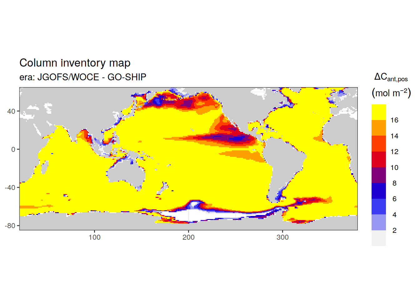
3.2.2 dCant inventory
# dCant inventory plot between 1994 to 2007
p_map_cant_inv(
  df = dcant_gruber_inv,
  var = "cant_inv")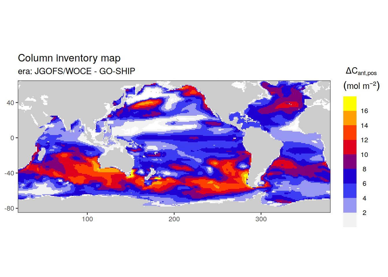
4 Cant plots in 2007
4.1 Horizontal plane maps
# Cant horizontal plane plot in year 2007
cant_annual_year <- cant_annual %>%
  filter(year == 2007) %>%
  mutate(depth = round(depth))

p_map_climatology(df = cant_annual_year, var = "cant")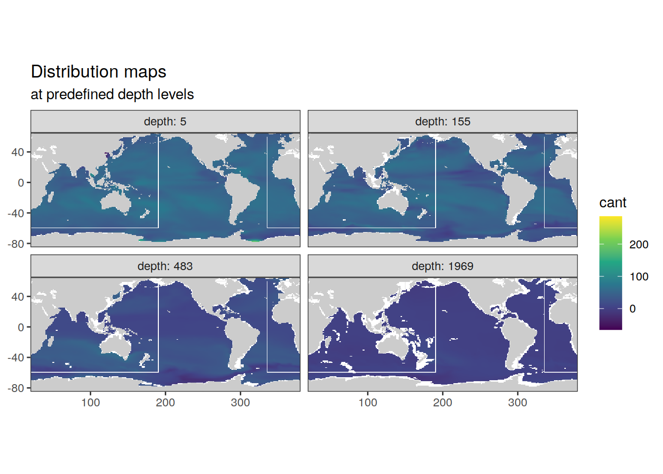
| Version | Author | Date |
|---|---|---|
| c3590c6 | Donghe-Zhu | 2020-12-18 |
4.2 Zonal mean section plot
# Cant zonal mean section plot in year 2007
for (i_basin_AIP in unique(cant_annual_zonal$basin_AIP)) {
  print(
    p_section_zonal(
      df = cant_annual_zonal %>% filter(basin_AIP == i_basin_AIP),
      var = "cant_mean",
      plot_slabs = "n",
      subtitle_text = paste("Basin:", i_basin_AIP)
    )
  )
}
| Version | Author | Date |
|---|---|---|
| c3590c6 | Donghe-Zhu | 2020-12-18 |

| Version | Author | Date |
|---|---|---|
| c3590c6 | Donghe-Zhu | 2020-12-18 |

| Version | Author | Date |
|---|---|---|
| c3590c6 | Donghe-Zhu | 2020-12-18 |
4.3 Global sections plot
# Cant global mean section plot in year 2007
cant_annual_year <- cant_annual %>%
  filter(year == 2007)

p_section_global(
  df = cant_annual_year,
  var = "cant",
  col = "divergent")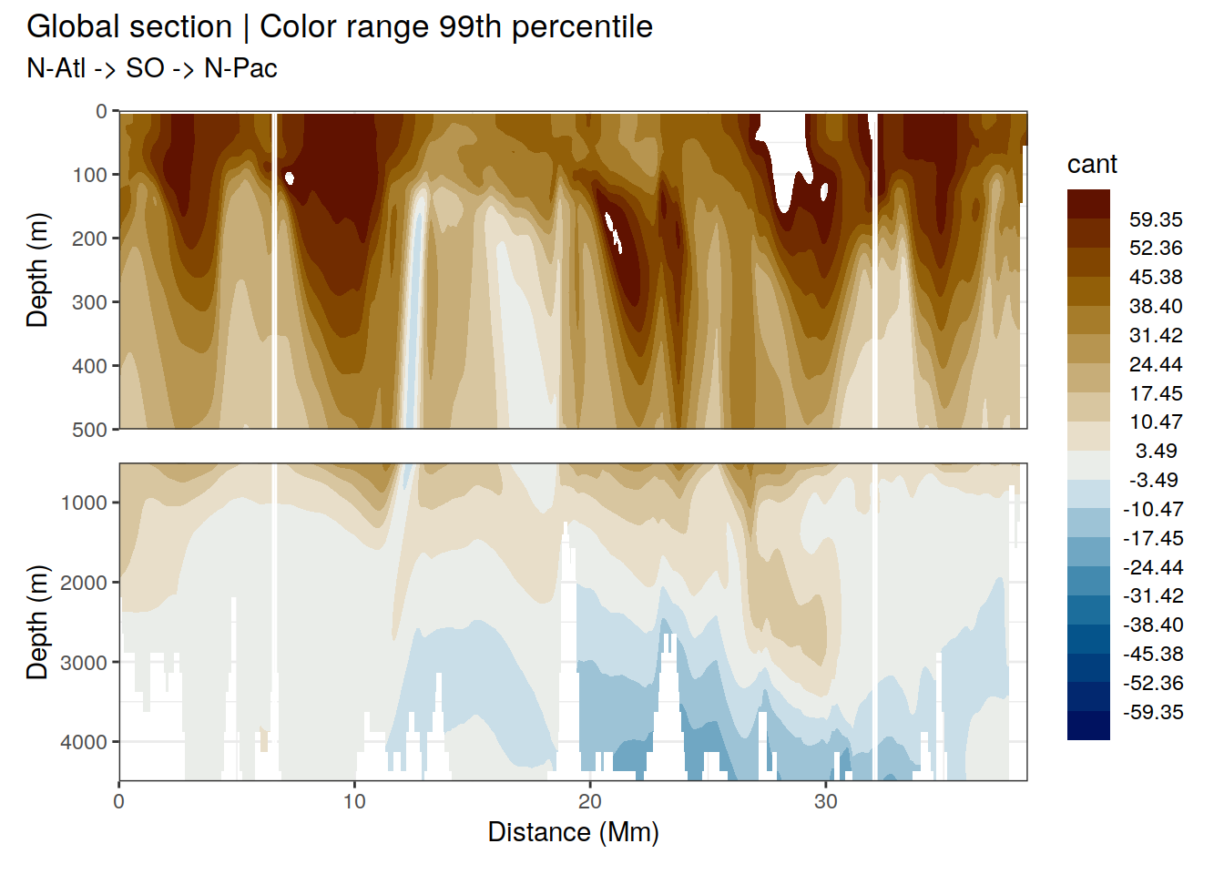
| Version | Author | Date |
|---|---|---|
| c3590c6 | Donghe-Zhu | 2020-12-18 |
5 dCant plots in 2007
5.1 Horizontal plane maps
# Cant horizontal plane plot in year 2007
dcant_gruber_round <- dcant_gruber %>%
  mutate(depth = round(depth))

p_map_climatology(df = dcant_gruber_round, var = "dcant")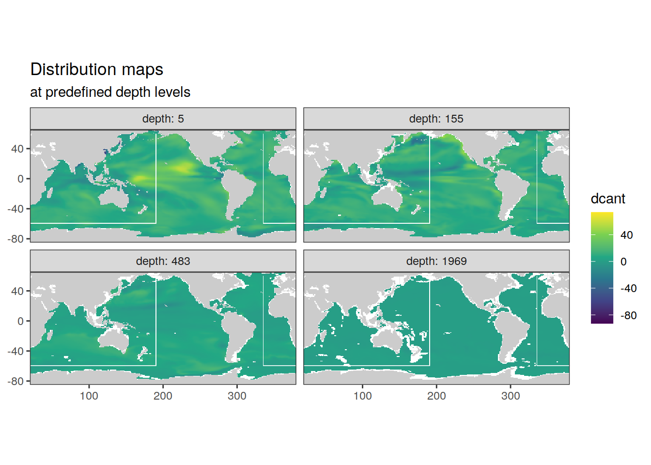
rm(dcant_gruber_round)5.2 Zonal mean section plot
# Cant zonal mean section plot in year 2007
for (i_basin_AIP in unique(dcant_gruber_zonal$basin_AIP)) {
  print(
    p_section_zonal(
      df = dcant_gruber_zonal %>% filter(basin_AIP == i_basin_AIP),
      var = "dcant_mean",
      plot_slabs = "n",
      subtitle_text = paste("Basin:", i_basin_AIP)
    )
  )
}


5.3 Global sections plot
# Cant global mean section plot in year 2007
p_section_global(
  df = dcant_gruber,
  var = "dcant",
  col = "divergent")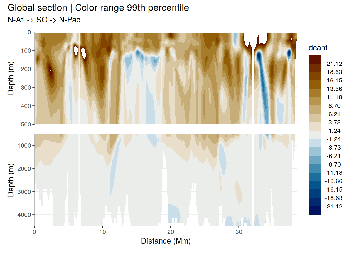
sessionInfo()R version 4.0.3 (2020-10-10)
Platform: x86_64-pc-linux-gnu (64-bit)
Running under: openSUSE Leap 15.1
Matrix products: default
BLAS: /usr/local/R-4.0.3/lib64/R/lib/libRblas.so
LAPACK: /usr/local/R-4.0.3/lib64/R/lib/libRlapack.so
locale:
[1] LC_CTYPE=en_US.UTF-8 LC_NUMERIC=C
[3] LC_TIME=en_US.UTF-8 LC_COLLATE=en_US.UTF-8
[5] LC_MONETARY=en_US.UTF-8 LC_MESSAGES=en_US.UTF-8
[7] LC_PAPER=en_US.UTF-8 LC_NAME=C
[9] LC_ADDRESS=C LC_TELEPHONE=C
[11] LC_MEASUREMENT=en_US.UTF-8 LC_IDENTIFICATION=C
attached base packages:
[1] stats graphics grDevices utils datasets methods base
other attached packages:
[1] gsw_1.0-5 testthat_2.3.2 stars_0.4-3 sf_0.9-6
[5] abind_1.4-5 tidync_0.2.4 metR_0.8.0 scico_1.2.0
[9] patchwork_1.1.0 collapse_1.4.2 forcats_0.5.0 stringr_1.4.0
[13] dplyr_1.0.2 purrr_0.3.4 readr_1.4.0 tidyr_1.1.2
[17] tibble_3.0.4 ggplot2_3.3.2 tidyverse_1.3.0 workflowr_1.6.2
loaded via a namespace (and not attached):
[1] fs_1.5.0 lubridate_1.7.9 httr_1.4.2
[4] rprojroot_1.3-2 tools_4.0.3 backports_1.1.10
[7] R6_2.5.0 KernSmooth_2.23-18 DBI_1.1.0
[10] colorspace_1.4-1 withr_2.3.0 tidyselect_1.1.0
[13] compiler_4.0.3 git2r_0.27.1 cli_2.1.0
[16] rvest_0.3.6 RNetCDF_2.4-2 xml2_1.3.2
[19] isoband_0.2.2 labeling_0.4.2 scales_1.1.1
[22] checkmate_2.0.0 classInt_0.4-3 digest_0.6.27
[25] rmarkdown_2.5 pkgconfig_2.0.3 htmltools_0.5.0
[28] dbplyr_1.4.4 rlang_0.4.8 readxl_1.3.1
[31] rstudioapi_0.11 farver_2.0.3 generics_0.0.2
[34] jsonlite_1.7.1 magrittr_1.5 ncmeta_0.3.0
[37] Matrix_1.2-18 Rcpp_1.0.5 munsell_0.5.0
[40] fansi_0.4.1 lifecycle_0.2.0 stringi_1.5.3
[43] whisker_0.4 yaml_2.2.1 grid_4.0.3
[46] blob_1.2.1 parallel_4.0.3 promises_1.1.1
[49] crayon_1.3.4 lattice_0.20-41 haven_2.3.1
[52] hms_0.5.3 knitr_1.30 pillar_1.4.6
[55] reprex_0.3.0 glue_1.4.2 evaluate_0.14
[58] RcppArmadillo_0.10.1.0.0 data.table_1.13.2 modelr_0.1.8
[61] vctrs_0.3.4 httpuv_1.5.4 cellranger_1.1.0
[64] gtable_0.3.0 assertthat_0.2.1 xfun_0.18
[67] lwgeom_0.2-5 broom_0.7.2 RcppEigen_0.3.3.7.0
[70] e1071_1.7-4 later_1.1.0.1 viridisLite_0.3.0
[73] class_7.3-17 ncdf4_1.17 units_0.6-7
[76] ellipsis_0.3.1