Analysis - others
Jens Daniel Müller and Donghe Zhu
13 January, 2021
Last updated: 2021-01-13
Checks: 7 0
Knit directory: emlr_mod_v_XXX/
This reproducible R Markdown analysis was created with workflowr (version 1.6.2). The Checks tab describes the reproducibility checks that were applied when the results were created. The Past versions tab lists the development history.
Great! Since the R Markdown file has been committed to the Git repository, you know the exact version of the code that produced these results.
Great job! The global environment was empty. Objects defined in the global environment can affect the analysis in your R Markdown file in unknown ways. For reproduciblity it’s best to always run the code in an empty environment.
The command set.seed(20200707) was run prior to running the code in the R Markdown file. Setting a seed ensures that any results that rely on randomness, e.g. subsampling or permutations, are reproducible.
Great job! Recording the operating system, R version, and package versions is critical for reproducibility.
Nice! There were no cached chunks for this analysis, so you can be confident that you successfully produced the results during this run.
Great job! Using relative paths to the files within your workflowr project makes it easier to run your code on other machines.
Great! You are using Git for version control. Tracking code development and connecting the code version to the results is critical for reproducibility.
The results in this page were generated with repository version d44f36f. See the Past versions tab to see a history of the changes made to the R Markdown and HTML files.
Note that you need to be careful to ensure that all relevant files for the analysis have been committed to Git prior to generating the results (you can use wflow_publish or wflow_git_commit). workflowr only checks the R Markdown file, but you know if there are other scripts or data files that it depends on. Below is the status of the Git repository when the results were generated:
Ignored files:
    Ignored:    .Rhistory
    Ignored:    .Rproj.user/

Unstaged changes:
    Modified:   analysis/_site.yml
    Modified:   code/Workflowr_project_managment.R
Note that any generated files, e.g. HTML, png, CSS, etc., are not included in this status report because it is ok for generated content to have uncommitted changes.
These are the previous versions of the repository in which changes were made to the R Markdown (analysis/analysis_others.Rmd) and HTML (docs/analysis_others.html) files. If you’ve configured a remote Git repository (see ?wflow_git_remote), click on the hyperlinks in the table below to view the files as they were in that past version.
| File | Version | Author | Date | Message |
|---|---|---|---|---|
| Rmd | d44f36f | Donghe-Zhu | 2021-01-13 | reorder analysis final |
1 Data sources
Cant estimates from this sensitivity case:
- Mean and SD per grid cell (lat, lon, depth)
- Zonal mean and SD (basin, lat, depth)
cant_3d <-
  read_csv(paste(path_version_data,
                 "cant_3d.csv",
                 sep = ""))

cant_zonal <-
  read_csv(paste(path_version_data,
                 "cant_zonal.csv",
                 sep = ""))

cant_predictor_zonal <-
  read_csv(paste(path_version_data,
                 "cant_predictor_zonal.csv",
                 sep = ""))
Target variable (cstar_tref) estimates from this sensitivity case:
- Mean and SD per grid cell (lat, lon, depth)
- Zonal mean and SD (basin, lat, depth)
target_3d <-
  read_csv(paste(path_version_data,
                 "target_3d.csv",
                 sep = ""))

target_zonal <-
  read_csv(paste(path_version_data,
                 "target_zonal.csv",
                 sep = ""))
Cleaned GLODAP-based synthetic model subsetting file as used in this sensitivity case
GLODAP <-
  read_csv(paste(
    path_version_data,
    "GLODAPv2.2020_MLR_fitting_ready.csv",
    sep = ""
  ))
2 Calculate gamma slab maps
cant_gamma_maps <- m_cant_slab(cant_3d)

cant_gamma_maps <- cant_gamma_maps %>%
  arrange(gamma_slab, eras)
3 Cant variability
3.1 Across models
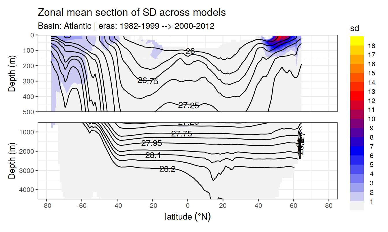
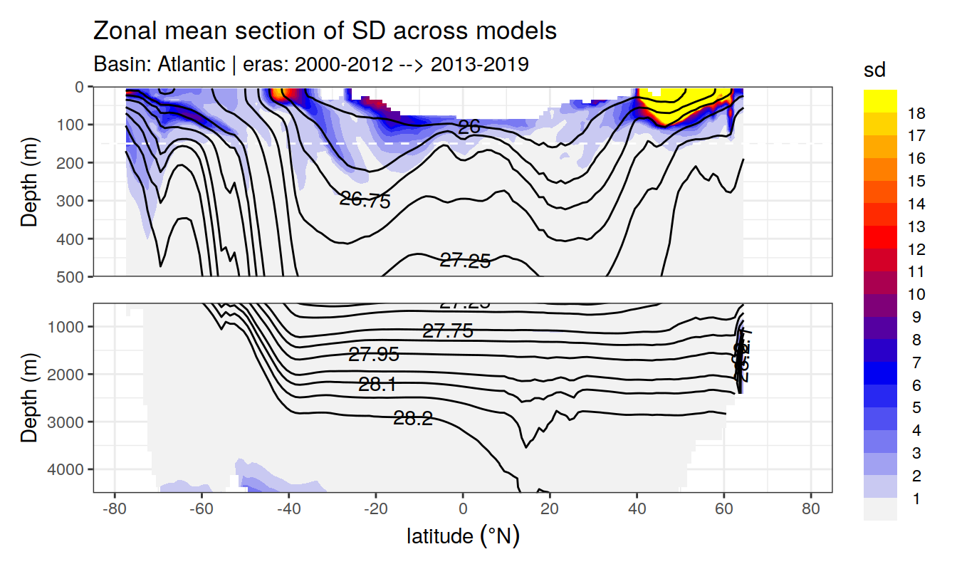
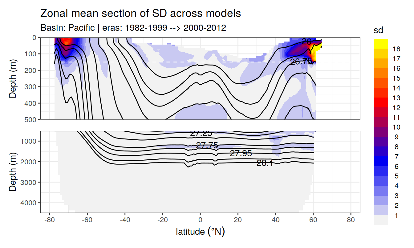
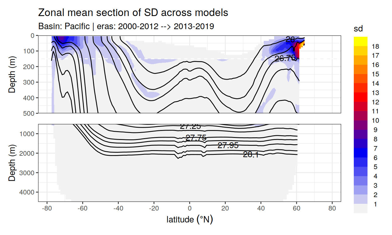
Standard deviation across Cant from all MLR models was calculate for each grid cell (XYZ). The zonal mean of this standard deviation should reflect the uncertainty associated to the predictor selection within each slab and era.
for (i_basin_AIP in unique(cant_zonal$basin_AIP)) {
  for (i_eras in unique(cant_zonal$eras)) {

    print(
      p_section_zonal(
        df = cant_zonal %>%
          filter(basin_AIP == i_basin_AIP,
                 eras == i_eras),
        var = "cant_sd_mean",
        gamma = "gamma_mean",
        legend_title = "sd",
        title_text = "Zonal mean section of SD across models",
        subtitle_text =
          paste("Basin:", i_basin_AIP, "| eras:", i_eras)
      )
    )

  }
}
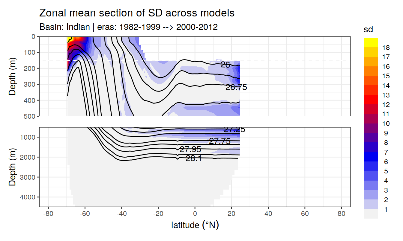
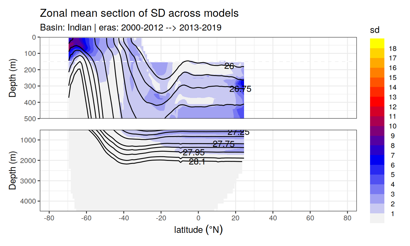
3.2 Across basins
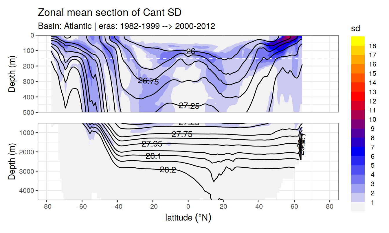
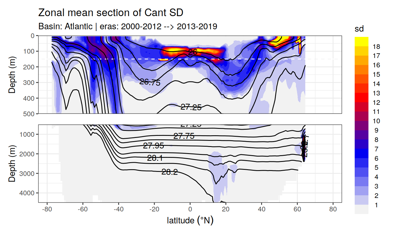
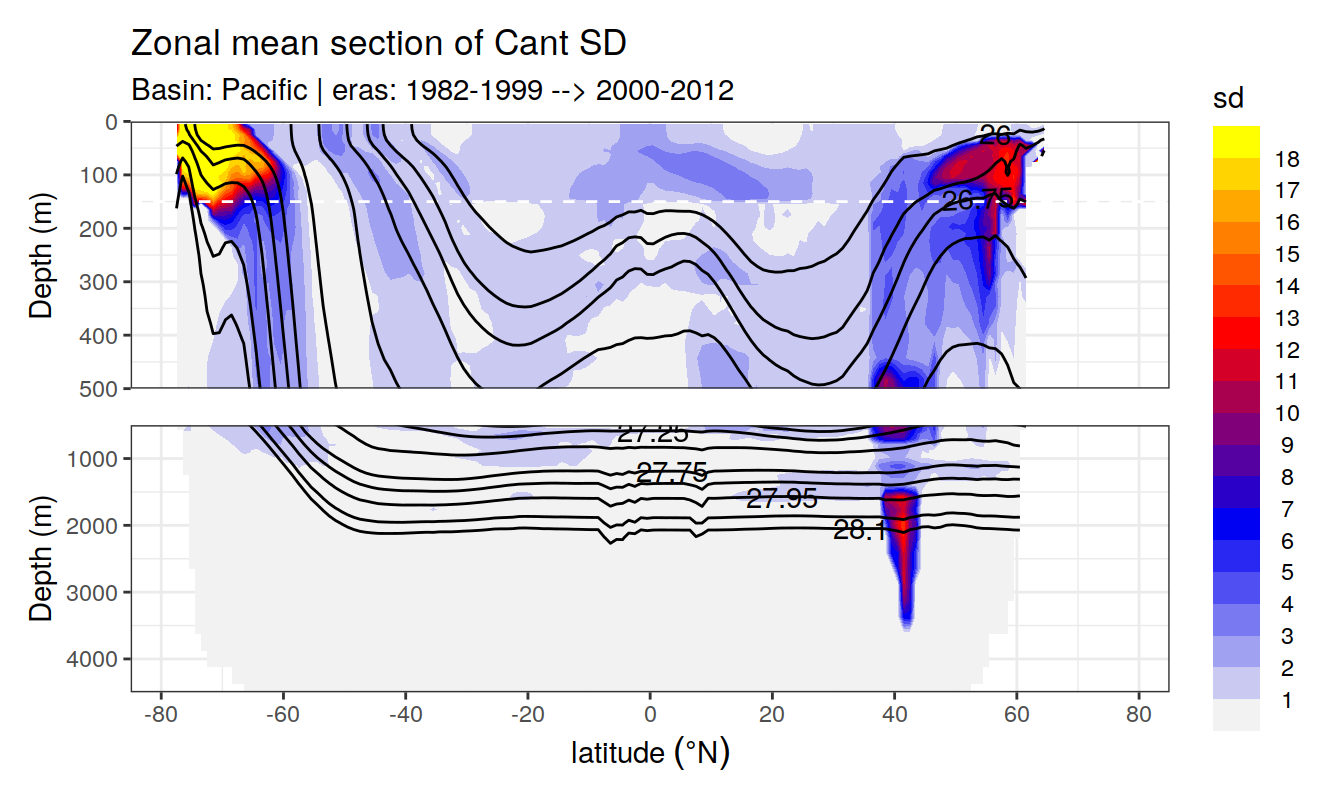
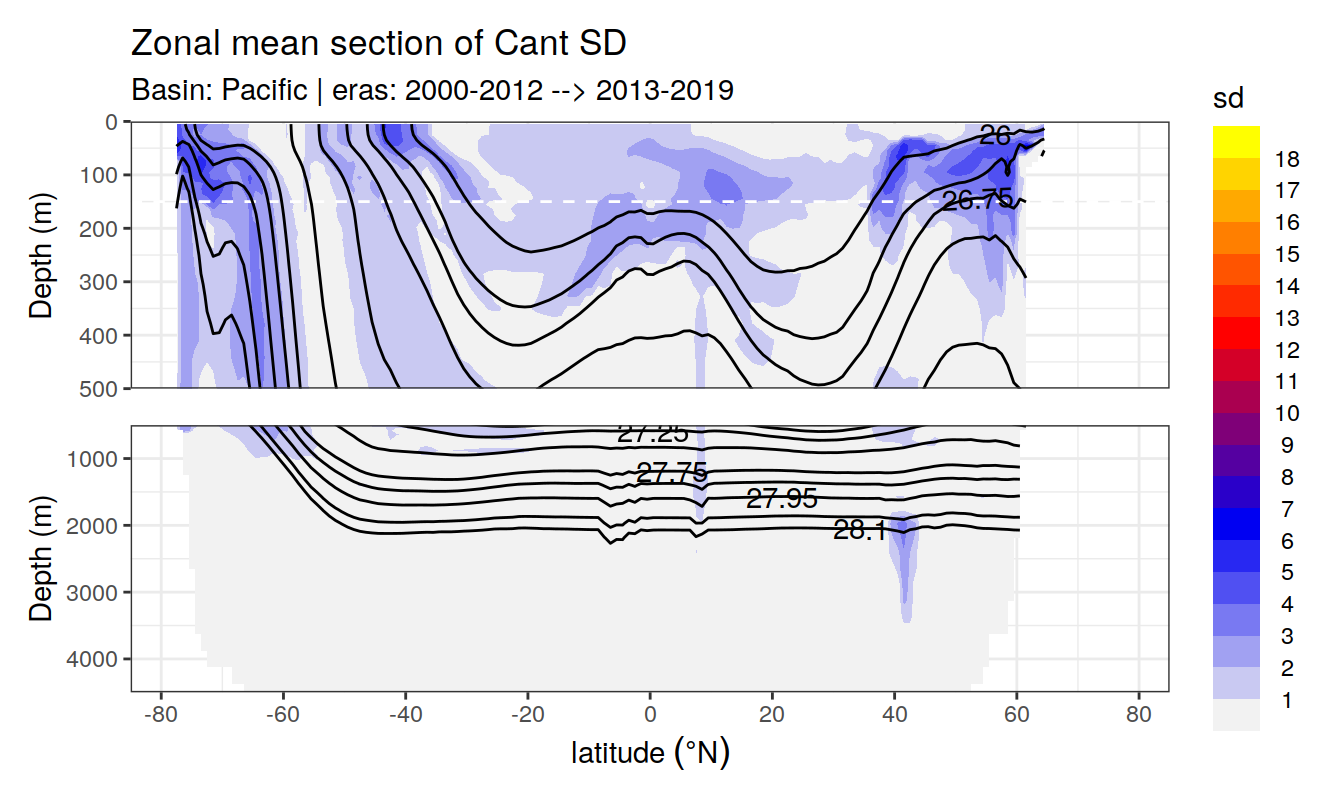
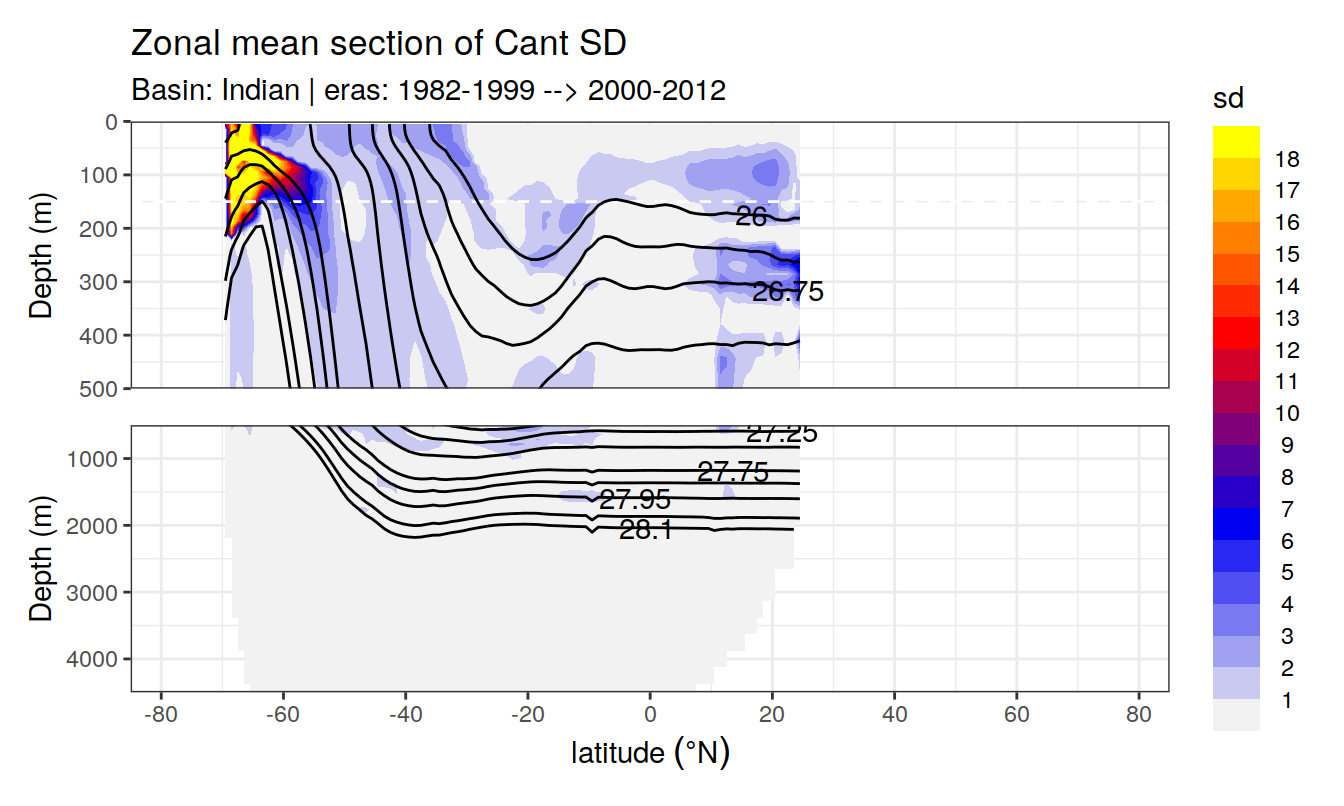
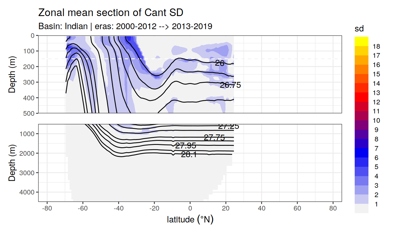
Standard deviation of mean cant values was calculate across all longitudes. This standard deviation should reflect the zonal variability of cant within the basin and era.
for (i_basin_AIP in unique(cant_zonal$basin_AIP)) {
  for (i_eras in unique(cant_zonal$eras)) {

    print(
      p_section_zonal(
        df = cant_zonal %>%
          filter(basin_AIP == i_basin_AIP,
                 eras == i_eras),
        var = "cant_sd",
        gamma = "gamma_mean",
        legend_title = "sd",
        title_text = "Zonal mean section of Cant SD",
        subtitle_text =
          paste("Basin:", i_basin_AIP, "| eras:", i_eras)
      )
    )

  }
}
3.3 Correlation
3.3.1 Cant vs model SD
3.3.1.1 Era vs basin
cant_3d %>%
  ggplot(aes(cant, cant_sd)) +
  geom_vline(xintercept = 0) +
  geom_hline(yintercept = 10) +
  geom_bin2d() +
  scale_fill_viridis_c(option = "magma",
                       direction = -1,
                       trans = "log10",
                       name = "log10(n)") +
  facet_grid(basin_AIP ~ eras)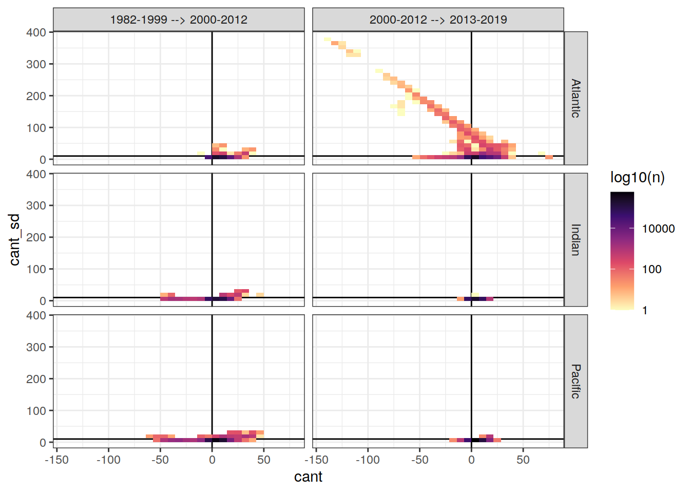
3.3.1.2 Basin vs gamma
cant_3d %>%
  ggplot(aes(cant, cant_sd)) +
  geom_vline(xintercept = 0) +
  geom_hline(yintercept = 10) +
  geom_bin2d() +
  scale_fill_viridis_c(option = "magma",
                       direction = -1,
                       trans = "log10",
                       name = "log10(n)") +
  facet_grid(gamma_slab ~ basin_AIP)
3.3.2 Cant vs regional SD
3.3.2.1 Era vs basin
cant_zonal %>%
  ggplot(aes(cant_mean, cant_sd)) +
  geom_vline(xintercept = 0) +
  geom_hline(yintercept = 10) +
  geom_bin2d() +
  scale_fill_viridis_c(option = "magma",
                       direction = -1,
                       trans = "log10",
                       name = "log10(n)") +
  facet_grid(basin_AIP ~ eras)
3.3.2.2 Era vs basin
cant_zonal %>%
  ggplot(aes(cant_mean, cant_sd)) +
  geom_vline(xintercept = 0) +
  geom_hline(yintercept = 10) +
  geom_bin2d() +
  scale_fill_viridis_c(option = "magma",
                       direction = -1,
                       trans = "log10",
                       name = "log10(n)") +
  facet_grid(gamma_slab ~ basin_AIP)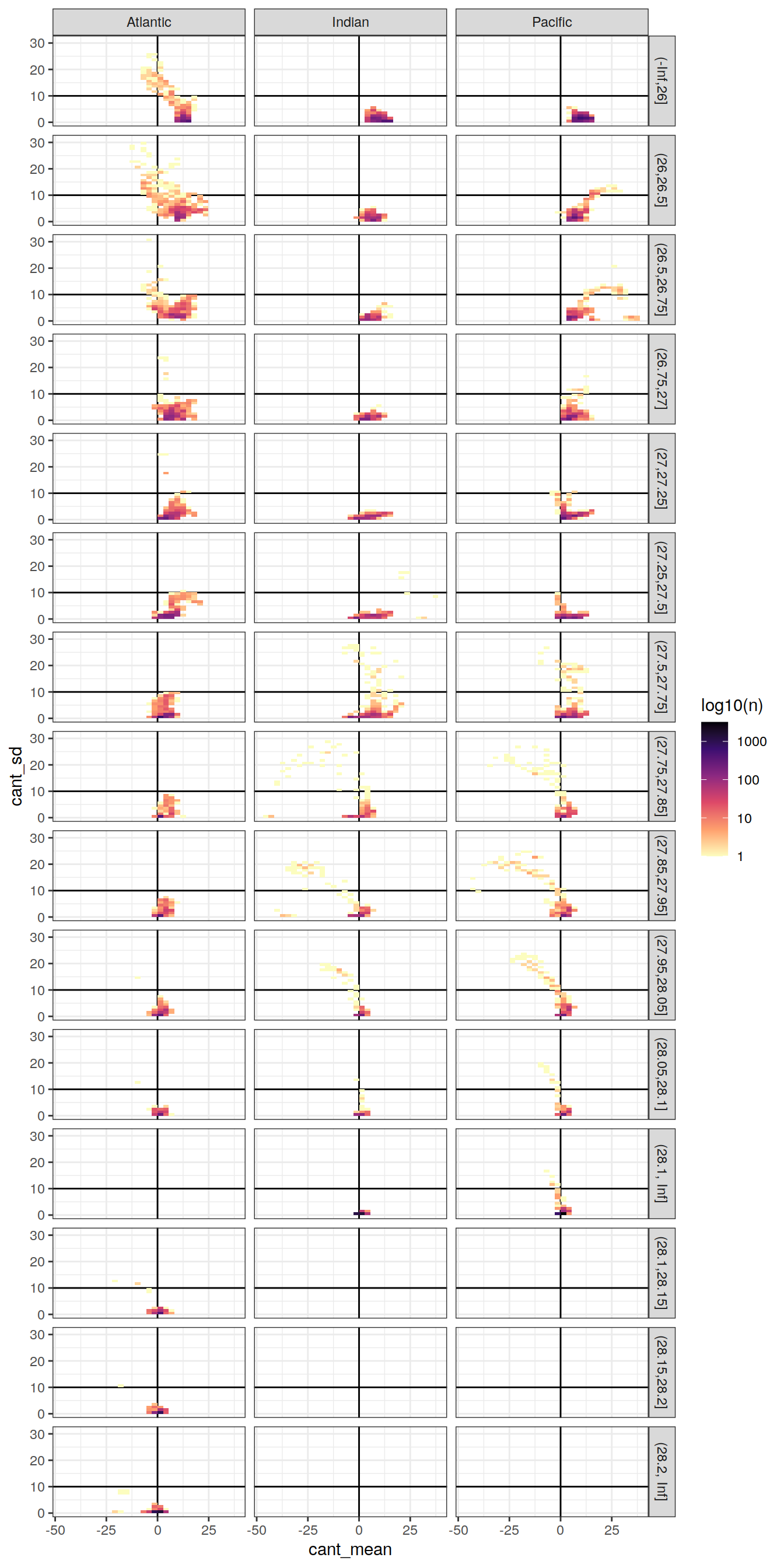
4 Cant - predictor contribution
for (i_var in paste("cant",
                    c("intercept", params_local$MLR_predictors),
                    sep = "_")) {
  print(
    p_section_zonal_divergent_gamma_eras_basin(df = cant_predictor_zonal,
                                               var = i_var,
                                               gamma = "gamma")
  )

}


rm(i_var)5 Neutral density
5.1 Slab depth
The plot below shows the depths of individual gamma slabs (color) together with the synthetic subsetting available in the respective slab.
Please note that:
- density slabs covering values >28.1 occur by definition only either in the Atlantic or Indo-Pacific basin
GLODAP_obs_coverage <- GLODAP %>%
  count(lat, lon, gamma_slab, era)

map +
  geom_raster(data = cant_gamma_maps,
              aes(lon, lat, fill = depth_max)) +
  geom_raster(data = GLODAP_obs_coverage,
              aes(lon, lat), fill = "red") +
  facet_grid(gamma_slab ~ era) +
  scale_fill_viridis_c(direction = -1) +
  theme(axis.ticks = element_blank(),
        axis.text = element_blank(),
        legend.position = "top")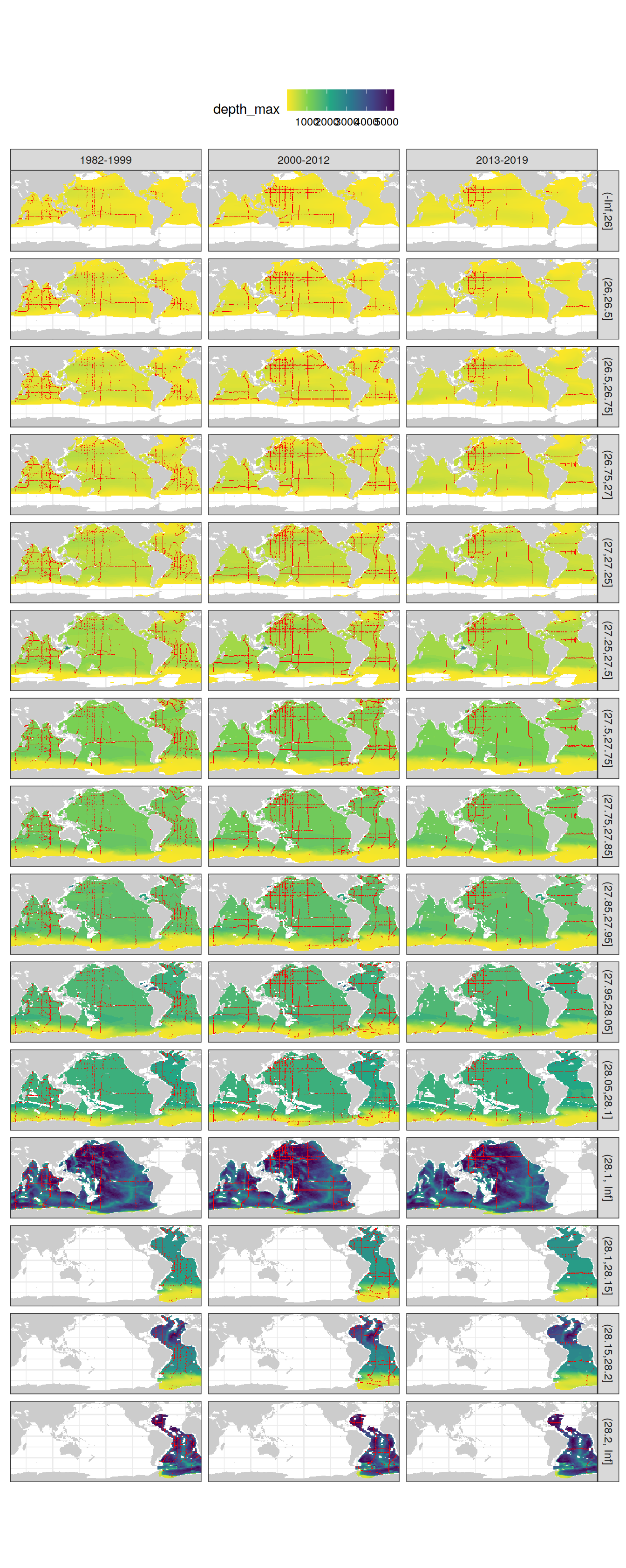
rm(GLODAP_obs_coverage)6 Target variable
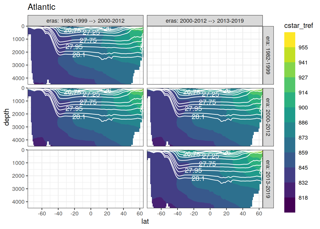
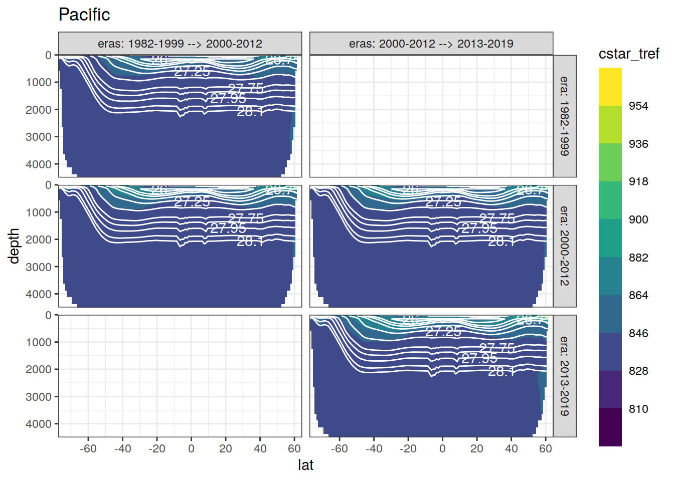
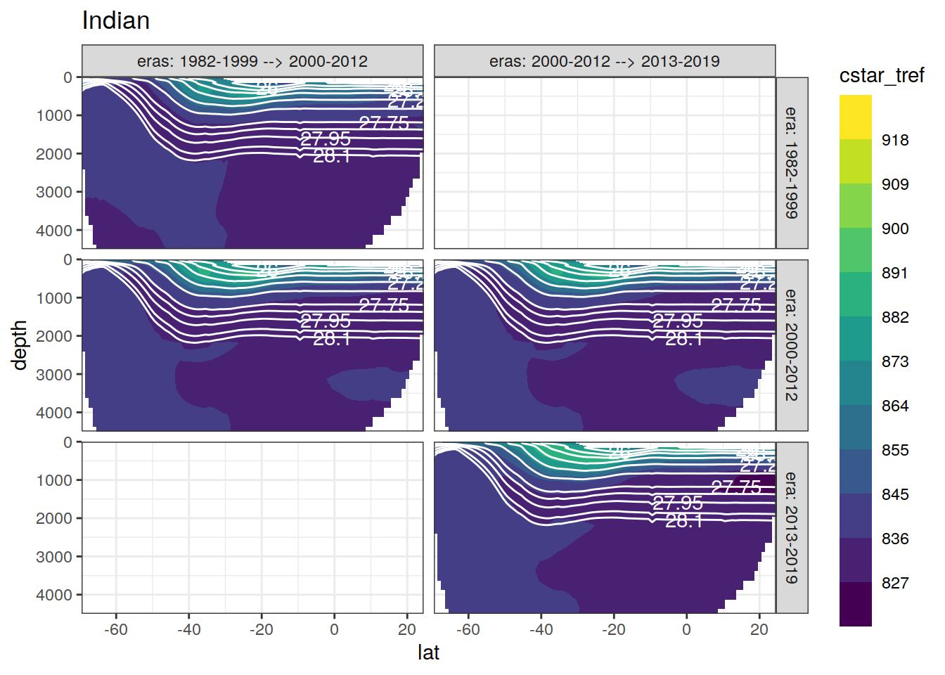
The predicted target variable (cstar_tref in this sensitivity case) is based on fitted MLRs and climatological fields of predictor variables, and calculated for each era.
6.1 Zonal mean sections
slab_breaks <- c(params_local$slabs_Atl[1:12], Inf)

for (i_basin_AIP in unique(target_zonal$basin_AIP)) {

  print(
  target_zonal %>%
    filter(basin_AIP == i_basin_AIP) %>%
    ggplot(aes(lat, depth,
               z = !!sym(
                 paste(params_local$MLR_target, "mean", sep = "_")
               ))) +
    geom_contour_filled(bins = 11) +
    scale_fill_viridis_d(name = params_local$MLR_target) +
    geom_contour(aes(lat, depth, z = gamma_mean),
                 breaks = slab_breaks,
                 col = "white") +
    geom_text_contour(
      aes(lat, depth, z = gamma_mean),
      breaks = slab_breaks,
      col = "white",
      skip = 1
    ) +
    scale_y_reverse() +
    coord_cartesian(expand = 0,
                    ylim = c(params_global$plotting_depth, 0)) +
    scale_x_continuous(breaks = seq(-100, 100, 20)) +
    guides(fill = guide_colorsteps(barheight = unit(10, "cm"))) +
    facet_grid(era ~ eras,
               labeller = labeller(.default = label_both)) +
    labs(title = i_basin_AIP)
  )

}
rm(slab_breaks)
sessionInfo()R version 4.0.3 (2020-10-10)
Platform: x86_64-pc-linux-gnu (64-bit)
Running under: openSUSE Leap 15.2
Matrix products: default
BLAS: /usr/local/R-4.0.3/lib64/R/lib/libRblas.so
LAPACK: /usr/local/R-4.0.3/lib64/R/lib/libRlapack.so
locale:
[1] LC_CTYPE=en_US.UTF-8 LC_NUMERIC=C
[3] LC_TIME=en_US.UTF-8 LC_COLLATE=en_US.UTF-8
[5] LC_MONETARY=en_US.UTF-8 LC_MESSAGES=en_US.UTF-8
[7] LC_PAPER=en_US.UTF-8 LC_NAME=C
[9] LC_ADDRESS=C LC_TELEPHONE=C
[11] LC_MEASUREMENT=en_US.UTF-8 LC_IDENTIFICATION=C
attached base packages:
[1] stats graphics grDevices utils datasets methods base
other attached packages:
[1] gt_0.2.2 kableExtra_1.3.1 marelac_2.1.10 shape_1.4.5
[5] scales_1.1.1 metR_0.9.0 scico_1.2.0 patchwork_1.1.1
[9] collapse_1.5.0 forcats_0.5.0 stringr_1.4.0 dplyr_1.0.2
[13] purrr_0.3.4 readr_1.4.0 tidyr_1.1.2 tibble_3.0.4
[17] ggplot2_3.3.3 tidyverse_1.3.0 workflowr_1.6.2
loaded via a namespace (and not attached):
[1] fs_1.5.0 lubridate_1.7.9 gsw_1.0-5
[4] webshot_0.5.2 httr_1.4.2 rprojroot_2.0.2
[7] tools_4.0.3 backports_1.1.10 R6_2.5.0
[10] DBI_1.1.0 colorspace_2.0-0 withr_2.3.0
[13] tidyselect_1.1.0 compiler_4.0.3 git2r_0.27.1
[16] cli_2.2.0 rvest_0.3.6 xml2_1.3.2
[19] isoband_0.2.3 labeling_0.4.2 checkmate_2.0.0
[22] digest_0.6.27 rmarkdown_2.5 oce_1.2-0
[25] pkgconfig_2.0.3 htmltools_0.5.0 dbplyr_1.4.4
[28] rlang_0.4.10 readxl_1.3.1 rstudioapi_0.13
[31] farver_2.0.3 generics_0.1.0 jsonlite_1.7.2
[34] magrittr_2.0.1 Matrix_1.2-18 Rcpp_1.0.5
[37] munsell_0.5.0 fansi_0.4.1 lifecycle_0.2.0
[40] stringi_1.5.3 whisker_0.4 yaml_2.2.1
[43] plyr_1.8.6 grid_4.0.3 blob_1.2.1
[46] parallel_4.0.3 promises_1.1.1 crayon_1.3.4
[49] lattice_0.20-41 haven_2.3.1 hms_0.5.3
[52] seacarb_3.2.14 knitr_1.30 pillar_1.4.7
[55] reprex_0.3.0 glue_1.4.2 evaluate_0.14
[58] RcppArmadillo_0.10.1.2.2 data.table_1.13.6 modelr_0.1.8
[61] vctrs_0.3.6 httpuv_1.5.4 testthat_3.0.1
[64] cellranger_1.1.0 gtable_0.3.0 assertthat_0.2.1
[67] xfun_0.20 broom_0.7.3 RcppEigen_0.3.3.9.1
[70] later_1.1.0.1 viridisLite_0.3.0 memoise_1.1.0
[73] ellipsis_0.3.1 here_1.0.1