Mapping cant

workflowr

• Summary
• Checks
• Past versions

Last updated: 2021-07-21

Checks: 7 0

Knit directory: emlr_obs_v_XXX/

This reproducible R Markdown analysis was created with workflowr (version 1.6.2). The Checks tab describes the reproducibility checks that were applied when the results were created. The Past versions tab lists the development history.

---

R Markdown file: up-to-date

Great! Since the R Markdown file has been committed to the Git repository, you know the exact version of the code that produced these results.

Environment: empty

Great job! The global environment was empty. Objects defined in the global environment can affect the analysis in your R Markdown file in unknown ways. For reproduciblity it’s best to always run the code in an empty environment.

Seed: set.seed(20200707)

The command set.seed(20200707) was run prior to running the code in the R Markdown file. Setting a seed ensures that any results that rely on randomness, e.g. subsampling or permutations, are reproducible.

Session information: recorded

Great job! Recording the operating system, R version, and package versions is critical for reproducibility.

Cache: none

Nice! There were no cached chunks for this analysis, so you can be confident that you successfully produced the results during this run.

File paths: relative

Great job! Using relative paths to the files within your workflowr project makes it easier to run your code on other machines.

Repository version: 78fe930

Great! You are using Git for version control. Tracking code development and connecting the code version to the results is critical for reproducibility.

The results in this page were generated with repository version 78fe930. See the Past versions tab to see a history of the changes made to the R Markdown and HTML files.

Note that you need to be careful to ensure that all relevant files for the analysis have been committed to Git prior to generating the results (you can use wflow_publish or wflow_git_commit). workflowr only checks the R Markdown file, but you know if there are other scripts or data files that it depends on. Below is the status of the Git repository when the results were generated:

Ignored files:
    Ignored:    .Rhistory
    Ignored:    .Rproj.user/

Unstaged changes:
    Modified:   code/Workflowr_project_managment.R

Note that any generated files, e.g. HTML, png, CSS, etc., are not included in this status report because it is ok for generated content to have uncommitted changes.

---

These are the previous versions of the repository in which changes were made to the R Markdown (analysis/mapping_dcant_mod_truth.Rmd) and HTML (docs/mapping_dcant_mod_truth.html) files. If you’ve configured a remote Git repository (see ?wflow_git_remote), click on the hyperlinks in the table below to view the files as they were in that past version.

File	Version	Author	Date	Message
html	971ce87	jens-daniel-mueller	2021-07-13	Build site.
Rmd	89d9fcb	jens-daniel-mueller	2021-07-13	complete revision
html	8d6c6c2	jens-daniel-mueller	2021-07-09	Build site.
Rmd	6743f76	jens-daniel-mueller	2021-07-09	complete revision

---

1 Version ID

The results displayed on this site correspond to the Version_ID: v_XXX

2 Required data

• tcant 3D fields at tref1 and tref2 for variable and constant climate model runs

tref  <-
  read_csv(paste(path_version_data,
                 "tref.csv",
                 sep = ""))

tcant_tref_1 <-
  read_csv(
    paste(
      path_model_preprocessing,
      "cant_annual_field_AD",
      "/cant_",
      unique(tref$median_year[1]),
      ".csv",
      sep = ""
    )
  )

tcant_tref_1 <- tcant_tref_1 %>%
  rename(tcant_tref_1 = cant_total) %>%
  select(-year)

tcant_tref_2 <-
  read_csv(
    paste(
      path_model_preprocessing,
      "cant_annual_field_AD",
      "/cant_",
      unique(tref$median_year[2]),
      ".csv",
      sep = ""
    )
  )

tcant_tref_2 <- tcant_tref_2 %>%
  rename(tcant_tref_2 = cant_total) %>%
  select(-year)

tcant_cc_tref_1 <-
  read_csv(
    paste(
      path_model_preprocessing,
      "cant_annual_field_CB",
      "/cant_",
      unique(tref$median_year[1]),
      ".csv",
      sep = ""
    )
  )

tcant_cc_tref_1 <- tcant_cc_tref_1 %>%
  rename(tcant_tref_1 = cant_total) %>%
  select(-year)

tcant_cc_tref_2 <-
  read_csv(
    paste(
      path_model_preprocessing,
      "cant_annual_field_CB",
      "/cant_",
      unique(tref$median_year[2]),
      ".csv",
      sep = ""
    )
  )

tcant_cc_tref_2 <- tcant_cc_tref_2 %>%
  rename(tcant_tref_2 = cant_total) %>%
  select(-year)

climatology <-
  read_csv(paste(path_model_preprocessing, "climatology_runA_2007.csv", sep = ""))

climatology <- climatology %>%
  select(lon,lat,depth, gamma)

3 dcant calculation

dcant_3d <- left_join(tcant_tref_1, tcant_tref_2) %>%
  mutate(dcant = tcant_tref_2 - tcant_tref_1)

rm(tcant_tref_1, tcant_tref_2)

dcant_3d <- dcant_3d %>%
  mutate(dcant_pos = if_else(dcant <= 0, 0, dcant))

dcant_3d <- full_join(dcant_3d, climatology)

dcant_3d <- m_cut_gamma(dcant_3d, "gamma")

dcant_3d_vc <- dcant_3d %>% 
  mutate(data_source = "mod_truth") %>% 
  select(lon, lat, depth, basin_AIP, data_source,
            tcant_tref_1, dcant, dcant_pos,
            gamma, gamma_slab)

dcant_3d <- left_join(tcant_cc_tref_1, tcant_cc_tref_2) %>%
  mutate(dcant = tcant_tref_2 - tcant_tref_1)

rm(tcant_cc_tref_1, tcant_cc_tref_2)

dcant_3d <- dcant_3d %>%
  mutate(dcant_pos = if_else(dcant <= 0, 0, dcant))

dcant_3d <- full_join(dcant_3d, climatology)

dcant_3d <- m_cut_gamma(dcant_3d, "gamma")

dcant_3d_cc <- dcant_3d %>% 
  mutate(data_source = "mod_truth_cc") %>% 
  select(lon, lat, depth, basin_AIP, data_source,
            tcant_tref_1, dcant, dcant_pos,
            gamma, gamma_slab)

rm(climatology, dcant_3d)

dcant_3d <- bind_rows(
  dcant_3d_cc,
  dcant_3d_vc
)

rm(
  dcant_3d_cc,
  dcant_3d_vc
)

4 Maps

dcant_3d %>%
  group_split(data_source) %>%
  # head(1) %>%
  map(~ p_map_climatology(
    df = .x,
    var = "dcant_pos",
    subtitle_text = paste("Climate: ", .x$data_source)
  ))

[[1]]

Past versions of cant_deep_climatology_map-1.png

Version	Author	Date
8d6c6c2	jens-daniel-mueller	2021-07-09

[[2]]

Past versions of cant_deep_climatology_map-2.png

Version	Author	Date
8d6c6c2	jens-daniel-mueller	2021-07-09

dcant_3d %>%
  group_split(data_source) %>%
  # head(1) %>%
  map(~ p_section_climatology_regular(
    df = .x,
    var = "dcant_pos",
    subtitle_text = paste("Climate: ", .x$data_source)
  ))

[[1]]

Past versions of cant_deep_climatology_sections-1.png

Version	Author	Date
8d6c6c2	jens-daniel-mueller	2021-07-09

[[2]]

Past versions of cant_deep_climatology_sections-2.png

Version	Author	Date
971ce87	jens-daniel-mueller	2021-07-13

5 Averaging and integration

5.1 Zonal sections

dcant_zonal <- dcant_3d %>%
  group_by(data_source) %>%
  nest() %>%
  mutate(zonal = map(.x = data, ~m_zonal_mean_sd(.x))) %>%
  select(-data) %>%
  unnest(zonal)


dcant_zonal <- m_cut_gamma(dcant_zonal, "gamma_mean")

5.2 Inventories

To calculate dcant column inventories, we:

1. Convert Cant concentrations to volumetric units
2. Multiply layer thickness with volumetric Cant concentration to get a layer inventory
3. For each horizontal grid cell and era, sum cant layer inventories for different inventory depths (100, 500, 1000, 3000, 10^{4} m)

Step 2 is performed separately for all Cant and positive Cant values only.

dcant_inv <- dcant_3d %>%
  group_by(data_source) %>%
  nest() %>%
  mutate(inv = map(.x = data, ~m_dcant_inv(.x))) %>%
  select(-data) %>%
  unnest(inv)

p_map_cant_inv(df = dcant_inv,
               var = "dcant_pos",
               subtitle_text = "for predefined integration depths") +
  facet_grid(inv_depth ~ data_source)

Past versions of calc_dcant_inventories-1.png

Version	Author	Date
971ce87	jens-daniel-mueller	2021-07-13
8d6c6c2	jens-daniel-mueller	2021-07-09

tcant_inv <- dcant_3d %>%
  rename(tcant = tcant_tref_1) %>%
  mutate(tcant_pos = if_else(tcant <= 0, 0, tcant)) %>% 
  group_by(data_source) %>%
  nest() %>%
  mutate(inv = map(.x = data, ~m_tcant_inv(.x))) %>%
  select(-data) %>%
  unnest(inv)

p_map_cant_inv(df = tcant_inv,
               var = "tcant_pos",
               breaks = seq(0,70,10),
               subtitle_text = "for predefined integration depths") +
  facet_grid(inv_depth ~ data_source)

Past versions of cant_total_inventories-1.png

Version	Author	Date
971ce87	jens-daniel-mueller	2021-07-13
8d6c6c2	jens-daniel-mueller	2021-07-09

5.3 Budgets

Global dcant budgets were estimated in units of Pg C. Please note that here we added dcant (all vs postitive only) values and do not apply additional corrections for areas not covered.

molC_to_PgC <- 12*1e-15

dcant_budget <- dcant_inv %>% 
  mutate(surface_area = earth_surf(lat, lon),
         dcant_grid = dcant*surface_area*molC_to_PgC,
         dcant_pos_grid = dcant_pos*surface_area*molC_to_PgC)

dcant_budget_global <- dcant_budget %>%
  group_by(data_source, inv_depth) %>% 
  summarise(dcant = sum(dcant_grid),
            dcant = round(dcant,1),
            dcant_pos = sum(dcant_pos_grid),
            dcant_pos = round(dcant_pos,1)) %>% 
  ungroup() %>% 
  pivot_longer(cols = dcant:dcant_pos,
               names_to = "estimate",
               values_to = "value")

dcant_budget_global %>%
  filter(inv_depth == params_global$inventory_depth_standard) %>%
  ggplot(aes(estimate, value)) +
  scale_fill_brewer(palette = "Dark2") +
  geom_col() +
  facet_grid(~data_source)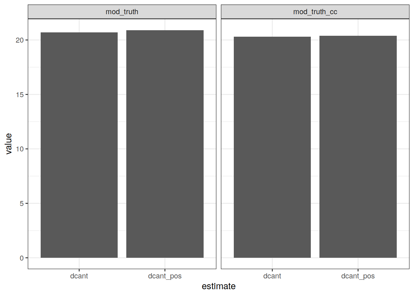

Past versions of budget_global-1.png

Version	Author	Date
971ce87	jens-daniel-mueller	2021-07-13

dcant_budget_basin_AIP <- dcant_budget %>% 
  group_by(basin_AIP, data_source, inv_depth) %>% 
  summarise(dcant = sum(dcant_grid),
            dcant = round(dcant,1),
            dcant_pos = sum(dcant_pos_grid),
            dcant_pos = round(dcant_pos,1)) %>% 
  ungroup() %>% 
  pivot_longer(cols = dcant:dcant_pos,
               names_to = "estimate",
               values_to = "value")

dcant_budget_basin_AIP %>%
  filter(inv_depth == params_global$inventory_depth_standard) %>%
  ggplot(aes(estimate, value, fill=basin_AIP)) +
  scale_fill_brewer(palette = "Dark2") +
  geom_col() +
  facet_grid(~data_source)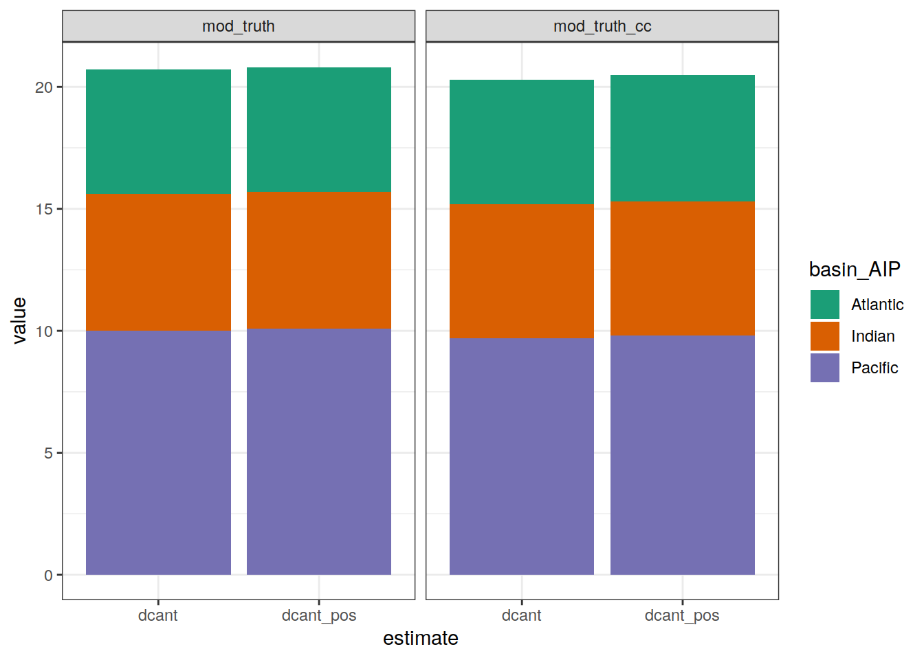

Past versions of budget_basin_AIP-1.png

Version	Author	Date
971ce87	jens-daniel-mueller	2021-07-13

dcant_budget_basin_MLR <-
  full_join(dcant_budget, basinmask) %>% 
  group_by(basin, MLR_basins, data_source, inv_depth) %>% 
  summarise(dcant = sum(dcant_grid),
            dcant = round(dcant,1),
            dcant_pos = sum(dcant_pos_grid),
            dcant_pos = round(dcant_pos,1)) %>% 
  ungroup() %>% 
  pivot_longer(cols = dcant:dcant_pos,
               names_to = "estimate",
               values_to = "value")

dcant_budget_basin_MLR %>%
  filter(inv_depth == params_global$inventory_depth_standard) %>%
  ggplot(aes(MLR_basins, value, fill=basin)) +
  geom_col() +
  facet_grid(estimate~data_source)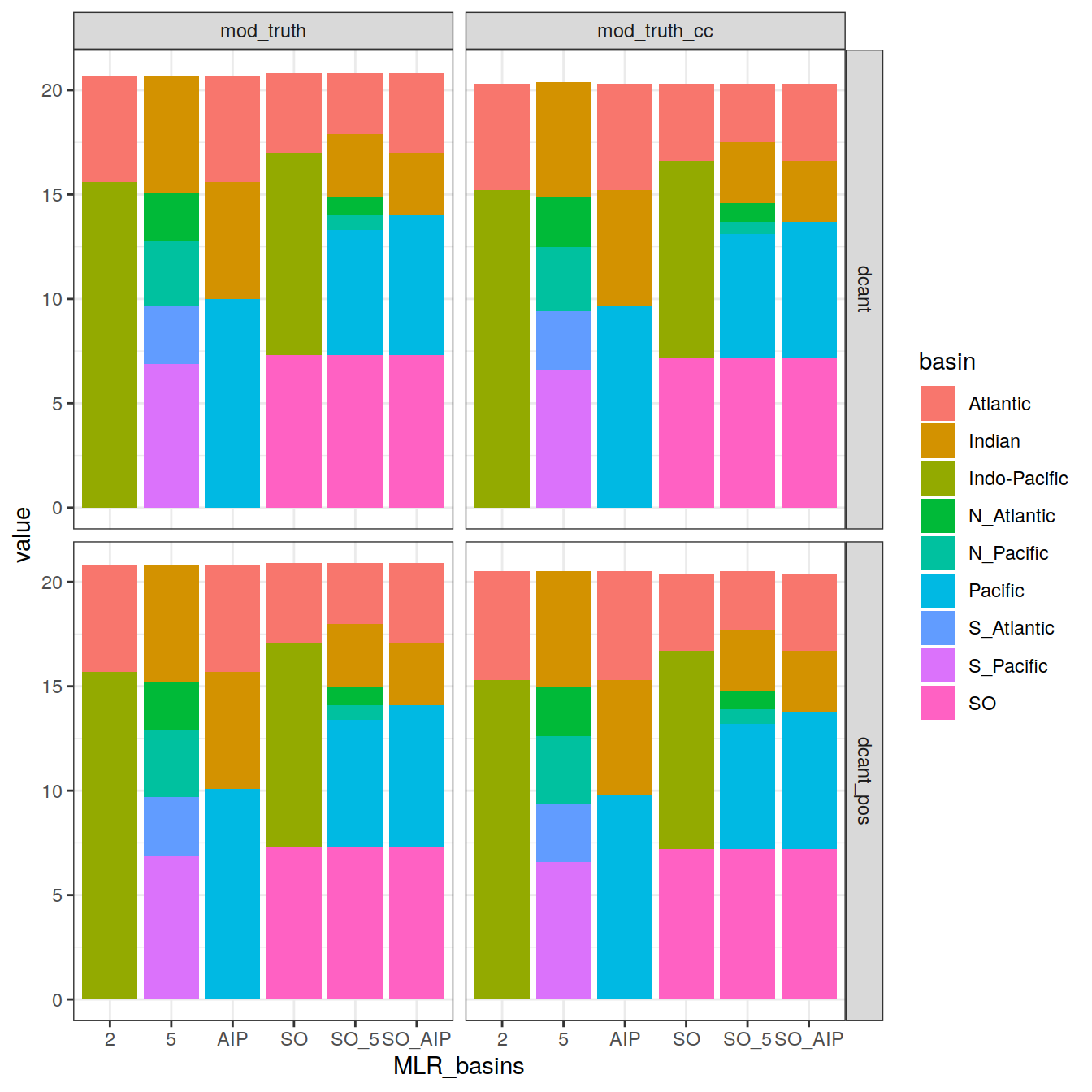

Past versions of budget_MLR_regions-1.png

Version	Author	Date
971ce87	jens-daniel-mueller	2021-07-13

dcant_budget_lat_grid <- 
  dcant_budget %>% 
  m_grid_horizontal_coarse() %>%
  group_by(lat_grid, basin_AIP, data_source, inv_depth) %>% 
  summarise(dcant = sum(dcant_grid),
            dcant = round(dcant,1),
            dcant_pos = sum(dcant_pos_grid),
            dcant_pos = round(dcant_pos,1)) %>% 
  ungroup() %>% 
  pivot_longer(cols = dcant:dcant_pos,
               names_to = "estimate",
               values_to = "value")

dcant_budget_lat_grid %>%
  filter(inv_depth == params_global$inventory_depth_standard) %>%
  ggplot(aes(lat_grid, value, fill = basin_AIP)) +
  geom_col() +
  scale_fill_brewer(palette = "Dark2") +
  coord_flip() +
  facet_grid(estimate ~ data_source)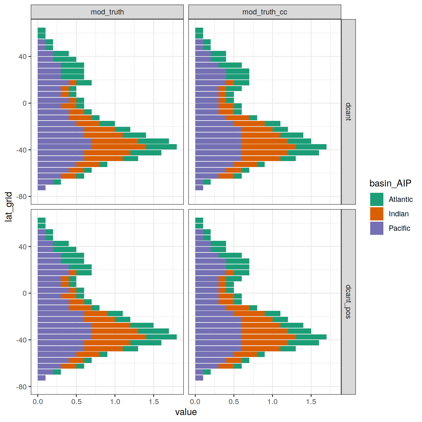

Past versions of budget_lat_grid-1.png

Version	Author	Date
971ce87	jens-daniel-mueller	2021-07-13

6 Alpha

6.1 3d fields

alpha_3d <- dcant_3d %>%
  mutate(
    alpha = dcant / tcant_tref_1,
    alpha = if_else(dcant <= 0 | tcant_tref_1 <= 0,
                    NaN, alpha)
  )

alpha_3d %>%
  filter(alpha < 1) %>%
  ggplot(aes(alpha)) +
  geom_histogram() +
  facet_grid(basin_AIP ~ data_source) +
  scale_x_continuous(breaks = seq(0, 1, 0.1))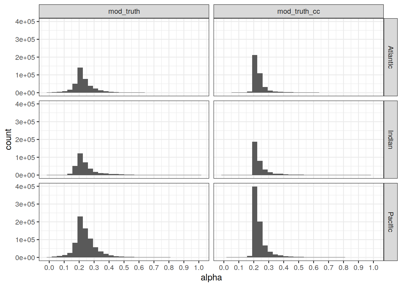

Past versions of alpha_3d-1.png

Version	Author	Date
8d6c6c2	jens-daniel-mueller	2021-07-09

median_alpha <- 
  alpha_3d %>% 
  group_by(depth, basin_AIP, data_source) %>% 
  summarise(alpha_median = median(alpha, na.rm = TRUE),
            alpha_mean = weighted.mean(alpha, tcant_tref_1, na.rm = TRUE)) %>% 
  ungroup()

alpha_3d %>%
  filter(alpha < 1) %>%
  ggplot(aes(alpha, depth)) +
  geom_bin2d(binwidth = c(0.01, 200)) +
  geom_path(data = median_alpha,
            aes(alpha_median, depth, col="Median")) +
  geom_path(data = median_alpha,
            aes(alpha_mean, depth, col="Weighted mean")) +
  scale_color_manual(name = "Alpha",
                     values = c("red", "orange")) +
  scale_y_reverse() +
  scale_x_continuous(breaks = seq(0, 1, 0.1),
                     limits = c(0,1)) +
  scale_fill_viridis_c(trans = "log10") +
  coord_cartesian(expand = 0) +
  facet_grid(basin_AIP~data_source)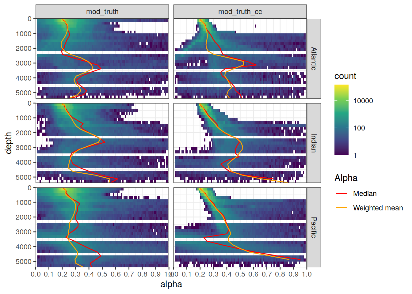

Past versions of alpha_3d-2.png

Version	Author	Date
8d6c6c2	jens-daniel-mueller	2021-07-09

print(paste("mean:",
            round(mean(
              alpha_3d$alpha, na.rm = TRUE
            ), 3)))

[1] "mean: 0.357"

print(paste("mean, weighted with Cant:",
            round(
              weighted.mean(
                x = alpha_3d$alpha,
                w = alpha_3d$tcant_tref_1,
                na.rm = TRUE
              ),
              3
            )))

[1] "mean, weighted with Cant: 0.216"

print(paste("median:",
            round(median(
              alpha_3d$alpha, na.rm = TRUE
            ), 3)))

[1] "median: 0.223"

6.2 Inventory maps

alpha_inv <- full_join(
  dcant_inv,
  tcant_inv)

alpha_inv <- alpha_inv %>% 
  mutate(alpha = dcant / tcant)


map +
  geom_raster(data = alpha_inv,
              aes(lon, lat, fill = alpha)) +
  facet_grid(inv_depth ~ data_source) +
  scale_fill_divergent(
    midpoint = median(alpha_inv$alpha)
  )

Past versions of alpha_surface_distribution-1.png

Version	Author	Date
8d6c6c2	jens-daniel-mueller	2021-07-09

7 Write csv

dcant_3d <- dcant_3d %>%
  select(-c(tcant_tref_1))

dcant_3d %>%
  filter(data_source == "mod_truth") %>%
  write_csv(paste(path_version_data,
                  "dcant_3d_mod_truth.csv", sep = ""))

dcant_3d %>%
  filter(data_source == "mod_truth_cc") %>%
  write_csv(paste(path_version_data,
                  "dcant_3d_mod_truth_cc.csv", sep = ""))



dcant_zonal %>%
  filter(data_source == "mod_truth") %>%
  write_csv(paste(path_version_data,
                  "dcant_zonal_mod_truth.csv", sep = ""))

dcant_zonal %>%
  filter(data_source == "mod_truth_cc") %>%
  write_csv(paste(path_version_data,
                  "dcant_zonal_mod_truth_cc.csv", sep = ""))



dcant_inv %>%
  filter(data_source == "mod_truth") %>%
  write_csv(paste(path_version_data,
                  "dcant_inv_mod_truth.csv", sep = ""))

dcant_inv %>%
  filter(data_source == "mod_truth_cc") %>%
  write_csv(paste(path_version_data,
                  "dcant_inv_mod_truth_cc.csv", sep = ""))



dcant_budget_global %>%
  filter(data_source == "mod_truth") %>%
  write_csv(paste(path_version_data,
                  "dcant_budget_global_mod_truth.csv", sep = ""))

dcant_budget_global %>%
  filter(data_source == "mod_truth_cc") %>%
  write_csv(paste(path_version_data,
                  "dcant_budget_global_mod_truth_cc.csv", sep = ""))

dcant_budget_basin_AIP %>%
  filter(data_source == "mod_truth") %>%
  write_csv(paste(path_version_data,
                  "dcant_budget_basin_AIP_mod_truth.csv", sep = ""))

dcant_budget_basin_AIP %>%
  filter(data_source == "mod_truth_cc") %>%
  write_csv(paste(path_version_data,
                  "dcant_budget_basin_AIP_mod_truth_cc.csv", sep = ""))

dcant_budget_basin_MLR %>%
  filter(data_source == "mod_truth") %>%
  write_csv(paste(path_version_data,
                  "dcant_budget_basin_MLR_mod_truth.csv", sep = ""))

dcant_budget_basin_MLR %>%
  filter(data_source == "mod_truth_cc") %>%
  write_csv(paste(path_version_data,
                  "dcant_budget_basin_MLR_mod_truth_cc.csv", sep = ""))

dcant_budget_lat_grid %>%
  filter(data_source == "mod_truth") %>%
  write_csv(paste(path_version_data,
                  "dcant_budget_lat_grid_mod_truth.csv", sep = ""))

dcant_budget_lat_grid %>%
  filter(data_source == "mod_truth_cc") %>%
  write_csv(paste(path_version_data,
                  "dcant_budget_lat_grid_mod_truth_cc.csv", sep = ""))

Session information

sessionInfo()

R version 4.0.3 (2020-10-10)
Platform: x86_64-pc-linux-gnu (64-bit)
Running under: openSUSE Leap 15.2

Matrix products: default
BLAS:   /usr/local/R-4.0.3/lib64/R/lib/libRblas.so
LAPACK: /usr/local/R-4.0.3/lib64/R/lib/libRlapack.so

locale:
 [1] LC_CTYPE=en_US.UTF-8       LC_NUMERIC=C              
 [3] LC_TIME=en_US.UTF-8        LC_COLLATE=en_US.UTF-8    
 [5] LC_MONETARY=en_US.UTF-8    LC_MESSAGES=en_US.UTF-8   
 [7] LC_PAPER=en_US.UTF-8       LC_NAME=C                 
 [9] LC_ADDRESS=C               LC_TELEPHONE=C            
[11] LC_MEASUREMENT=en_US.UTF-8 LC_IDENTIFICATION=C       

attached base packages:
[1] stats     graphics  grDevices utils     datasets  methods   base     

other attached packages:
 [1] marelac_2.1.10  shape_1.4.5     ggforce_0.3.3   metR_0.9.0     
 [5] scico_1.2.0     patchwork_1.1.1 collapse_1.5.0  forcats_0.5.0  
 [9] stringr_1.4.0   dplyr_1.0.5     purrr_0.3.4     readr_1.4.0    
[13] tidyr_1.1.2     tibble_3.0.4    ggplot2_3.3.3   tidyverse_1.3.0
[17] workflowr_1.6.2

loaded via a namespace (and not attached):
 [1] fs_1.5.0                 lubridate_1.7.9          gsw_1.0-5               
 [4] RColorBrewer_1.1-2       httr_1.4.2               rprojroot_2.0.2         
 [7] tools_4.0.3              backports_1.1.10         R6_2.5.0                
[10] DBI_1.1.0                colorspace_1.4-1         withr_2.3.0             
[13] tidyselect_1.1.0         compiler_4.0.3           git2r_0.27.1            
[16] cli_2.1.0                rvest_0.3.6              xml2_1.3.2              
[19] isoband_0.2.2            labeling_0.4.2           scales_1.1.1            
[22] checkmate_2.0.0          digest_0.6.27            rmarkdown_2.5           
[25] oce_1.2-0                pkgconfig_2.0.3          htmltools_0.5.0         
[28] dbplyr_1.4.4             rlang_0.4.10             readxl_1.3.1            
[31] rstudioapi_0.11          farver_2.0.3             generics_0.0.2          
[34] jsonlite_1.7.1           magrittr_1.5             Matrix_1.2-18           
[37] Rcpp_1.0.5               munsell_0.5.0            fansi_0.4.1             
[40] lifecycle_1.0.0          stringi_1.5.3            whisker_0.4             
[43] yaml_2.2.1               MASS_7.3-53              grid_4.0.3              
[46] blob_1.2.1               parallel_4.0.3           promises_1.1.1          
[49] crayon_1.3.4             lattice_0.20-41          haven_2.3.1             
[52] hms_0.5.3                seacarb_3.2.14           knitr_1.30              
[55] pillar_1.4.7             reprex_0.3.0             glue_1.4.2              
[58] evaluate_0.14            RcppArmadillo_0.10.1.2.0 data.table_1.13.2       
[61] modelr_0.1.8             vctrs_0.3.5              tweenr_1.0.2            
[64] httpuv_1.5.4             testthat_2.3.2           cellranger_1.1.0        
[67] gtable_0.3.0             polyclip_1.10-0          assertthat_0.2.1        
[70] xfun_0.18                broom_0.7.5              RcppEigen_0.3.3.7.0     
[73] later_1.1.0.1            viridisLite_0.3.0        ellipsis_0.3.1          
[76] here_0.1